Prognosis aims at estimating the remaining useful life (RUL for short) of a system or a component in ser- vice. The RUL of a system corresponds to the remain-.
A generic adaptive prognostic function for heterogeneous multi-component systems : application to helicopters ´ Bensana Pauline Ribot and Eric Onera - The French Aerospace Lab F-31055, Toulouse, France
ABSTRACT: The Helimaintenance project aims at optimizing the maintenance of civil helicopters. An embedded supervision system is in charge of monitoring the helicopter and detecting problems which require maintenance actions. A data processing system integrating a prognostic function receives information from the supervision system and suggests component replacements before they fail and cause a system failure. In this paper we propose a hybrid component-oriented model for a heterogeneous physical system. The model describes the evolution of the health condition of the system over time from the available knowledge on behaviour and degradation of components. A generic adaptive prognostic function is developed and provides a common support for the maintenance decision of a heterogeneous multi-component system. It computes faults probabilities of components by using the parametrized Weibull model and updates these probabilities according to new data like on-line diagnostic result or new measurements. For illustration, the prognostic function is then applied on an example of a helicopter subsystem.
1
INTRODUCTION
Maintenance efficiency of industrial systems is an important economical issue as it is a way to improve reliability and safety while reducing the final cost of systems. The Helimaintenance project aims at optimizing the maintenance of helicopters. The objective is to develop an integrated logistics system in order to support the scheduling of maintenance actions and reduce the unavailability of helicopters. Maintenance actions must be decided on an efficient and complete analysis of the health of the system when it is operating. An embedded supervision system is in charge of monitoring the helicopter and detecting problems and misbehaviors which require maintenance actions. The supervision system integrates a diagnostic function to accurately determine which components may cause a system failure and have to be replaced by a maintenance action. In order to optimize the maintenance cost, it is also necessary to perform preventive maintenance by deciding to act on the system before the problems actually occur. A prognostic reasoning must be performed over the system to establish whether a preventive action is pertinent at a given time. Prognosis aims at estimating the remaining useful life (RUL for short) of a system or a component in service. The RUL of a system corresponds to the remaining time until the system cannot successfully perform
a particular function anymore and must be replaced (Engel et al. 2000). This temporal prediction relies on knowledge about component aging that is contained in a prognostic model (Gorjian et al. 2009). In the literature, several prognostic approaches already exist which rely on different models (Roemer et al. 2005, Schwabacher and Goebel 2007, Dragomir et al. 2009). Experience-based approaches, like case-based reasoning or reliability analyses, are the only alternative when no physical knowledge of the system is available. They allow to determine the failure probability at a given time in the future from a failure history. When on-line observations (i.e. measurements) are accessible, learning or on-line estimation methods (trend monitoring methods) can be used to evaluate the degradation state of the system. Model-based prognostic approaches are based on a deep knowledge of the system and rely on a continuous model represented as a set of equations which involve physical quantities (like humidity, temperature, etc.) corresponding to environmental constraints of the system (Saxena et al. 2008). The choice of a prognostic method depends on the available knowledge of the system, the presence of sensors or models that allow to monitor and to analyze the real condition of the system. Classical reliability methods can be used to compute the RUL of components but they do not take into account the real stress of the supervised system when
it is operating. A stress can result from a fault within the system or an abnormal solicitation (like mechanical vibrations, thermal impacts, etc.) that can accelerate the component aging and thus affect the system RUL. An adaptive method is then required to take into account the current condition of the system that is evaluated by the diagnostic function and by monitoring environmental conditions (Kacprzynsk et al. 2004, Kirkland et al. 2004). In this paper we propose an adaptive prognostic function that receives information from the supervision system (measures from embedded sensors and diagnosis results) and suggests component replacements before they cause a system failure. Aeronautical systems, like helicopters, are complex systems built from an assemblage of heterogeneous components. Section 2 recalls the formal modeling framework developed in Ribot et al. (2009) for an heterogeneous multi-component system that allows to describe the behavior and the degradation of components. Section 3 proposes a generic adaptive prognostic function that computes fault probabilities of components by using the parametrized Weibull model and updates these probabilities according to new data like on-line diagnostic result or new measurements in order to evaluate the RUL of components. For illustration, the prognostic function is finally applied to an example of a helicopter subsystem in Section 4. 2
GENERIC MODELING FRAMEWORK
A multi-component system is built from an assemblage of heterogeneous components. It is then modeled as a set of N interacting components: Comps = {C 1 , ..., C N }. The knowledge for each component that will be used by the prognostic function is represented in a abstract but homogeneous way.
be differential, algebraic or logical. Therefore a component C i is formally defined by a 3-tuple C i = hP i , Ri , Ai i, where P i = {pi,k } is the set of component parameters, Ri = {r(pi,k )} is the set of parameter ranges and Ai = {ari,k } is the set of relations between parameters. The multi-component system Σ is modeled as a set of N components that interact in order to perform some specific functions. The system description must then be refined to take the interactions between components into account. 2.2 Structural model The structural model describes the possible set of interactions between components that are usually modeled with ports which can exchange data flow in the real system. In this framework, such ports are represented by some component parameters. A connection is then defined as the association of parameters from different components. The structural model of the sysSt tem is given by the function St : P −→ 2P that is defined such that St(op) 3 ip represents a data flow coming from the parameter op and going to the set of parameters ip (Ribot et al. 2011). Let OP ⊂ P denote the set of parameters op such that St(op) is defined, let IP ⊆ P \ OP denote the set of parameters ip such that ∃op ∈ OP, ip ∈ St(op). Based on the structural model St, the set of parameters P i of a component C i can then be partitioned into three subsets: input parameters, output parameters and private parameters. • The set of input parameters is defined by IP i = P i ∩ IP. The value of an input parameter ipi,k ∈ IP i is determined by a connection with another component. The mechanisms implemented by the component C i cannot modify its value, so the value of ipi,k is not fixed by any relation ari,k of C i.
2.1 Multi-component system A component C i can always be characterized by a set of physical quantities that are represented by a set of parameters denoted P i . A parameter in P i is then a continuous or discrete variable of the component model. The k-th parameter in P i is denoted pi,k and its value at time t is denoted pi,k (t). Each parameter pi,k is associated to a set of admissible values denoted r(pi,k ) called the range. For instance, the range can be an interval of real numbers for a continuous parameter or {0, 1} for a boolean parameter. The value of a physical quantity may depend on the other component quantities. A set of relations denoted Ai represents how these values are linked in a component C i . A relation ari,k ∈ Ai is then written as pi,k = ari,k (pi,j , . . . , pi,l ),
(1)
where {pi,j , . . . , pi,l } ⊆ P i . The value of the parameter pi,k is determined by the relation ari,k that can
• The set of output parameters is defined by OP i = P i ∩ OP. The value of an output parameter opi,k ∈ OP i results from the mechanisms implemented by C i and its inputs, so it is determined by at least a relation ari,k of C i . • The set of private parameters is defined by PP i = P i \ (OP i ∪ IP i ). A private parameter ppi,k ∈ PP i represents an internal characteristic, specific to the component that can be modified by the mechanisms implemented by C i . Private parameters are used to model the faults and the component aging for diagnosis and prognosis purposes. Figure 1 represents the structural model of a system composed of two interacting components {C 1 , C 2 } with St(op1,1 ) = ip2,1 represented by the oriented connector.
op1,1
ip1,1 ip1,2
ip2,1 ar
ar 1 ,1
pp1,1
pp2,1
C1
2 ,1
pp2,2
op2,1 C2
Figure 1: Component and interaction modeling with parameters
In nominal mode, C i provides the basic functions whose functional conditions are given by the set Ain . If one parameter pi,k has a value out of its nominal range, the functional conditions depending on pi,k are not satisfied and, consequently, the associated functions are not available. The component is either in a fault mode or in abnormal mode.
2.3 Functional model A system is usually designed in order to provide some applications. To perform these applications, each system component C i supports a set of basic functions denoted FU i . These basic functions rely on the nominal behavior of components that comes from the design stage and are modeled as functional conditions. A functional condition associated to a basic function F ui,k ∈ FU i is defined as follows: F ui,k ≡ (opi,k = ari,k (ipi,j , . . . , ipi,l , ppi,m , . . . , ppi,n )) i,k
i
i,j
i,l
i
where op ∈ OP , {ip , . . . , ip } ⊆ IP and {ppi,m , . . . , ppi,n } ⊆ PP i . A basic function is available on a component if the constraint of its associated functional condition is satisfied. The functional model of a multi-component system defines the set of basic functions implemented by components that are required to perform the system applications. 2.4 Operational modes Some operational modes can be defined for a component C i according to the set of basic functions available on this component. The model of the component C i in a mode mix is defined by Cxi = hP i , Rix , Aix i
(2)
with P i = {pi,k }, the set of component parameters (supposed to be fixed), Rix = {rx (pi,k )}, the set of ranges for parameters in the mode mix and Aix = {arxi,k }, the set of relations defined for the mode mix . The behavior of a component C i in mode mix at time t is given by Cxi with � ∀arxi,k ∈ Aix , opi,k (t) = arxi,k (pi,j (t), ..., pi,l (t)) ∀pi,k ∈ P i , pi,k (t) ∈ rx (pi,k ). Based on the functional state and the knowledge about component behavior, it is possible to distinguish three kinds of operational modes for a component: nominal mode, fault mode and abnormal mode. 2.4.1 Nominal mode The nominal mode min for a component C i is unique and describes the nominal behaviors. It is modeled by Cni = hP i , Rin , Ain i with � ∀arni,k ∈ Ain , opi,k (t) = arni,k (pi,j (t), . . . , pi,l (t)) ∀pi,k ∈ P i , pi,k (t) ∈ rn (pi,k ).
2.4.2 Fault mode A fault mode of a component is an operational mode with an explicit model. The faulty behavior is associated to the value of a private parameter that is out of its nominal range. For a given fault f , a fault mode mif for a component C i at time t is defined by the model Cfi = hP i , Rif , Aif i so that ∃ppi,k ∈ PP i , ppi,k (t) ∈ / rn (ppi,k ).
(3)
A fault is assumed to be persistent as it results from a problem within the component. 2.4.3 Abnormal mode An abnormal solicitation of a component may also cause some function losses. This corresponds to an abnormal mode that is not necessarily represented by a model, but characterized by a value of an input parameter that is out of its nominal range. A component C i is in an abnormal mode mia at time t if ∃ipi,k ∈ IP i , ipi,j (t) 6∈ rn (ipi,k ).
(4)
An abnormal solicitation may be intermittent. Thus, a component can return in nominal mode as soon as the value of the input parameter representing this solicitation is in nominal range again. In an abnormal mode, some private parameters of the component may also be out of nominal ranges. The component is then in an abnormal faulty mode that is denoted miaf . 2.4.4 Mode automaton A set of operational modes is associated to a component C i : Mi = {min , mia1 , . . . , mif1 , . . . , miaf1 , . . . , miafk } where each mode mix is characterized by a model Cxi if the knowledge on the behavior of components is available. During the system operation, the mode of a component C i changes each time a fault or an abnormal solicitation occurs on it. The mode of a component C i at time t is denoted mode(C i , t). So, along the operation time, from t0 till t, the component follows a trajectory of modes mode(C i , t0 ).mode(C i , t1 ) . . . mode(C i , t). Very often, the component is in nominal mode at t0 , then mode(C i , t0 ) = min (all the parameters are in nominal range defined by the nominal model). The last mode of the trajectory is a fault mode mip in which all basic
functions are no longer available on C i . The different possible changes of modes for a component C i can be described by a mode automaton as illustrated in Figure 2. The automaton states represent the component modes in Mi and the transitions correspond to fault or abnormal events (generated when a private or an input parameter evolves out of nominal range). m ifi fi
f1
mni a1
m ai 1
f1
PROGNOSIS METHODOLOGY
The difficulty is to establish a common prognostic representation whatever the type of available knowledge about component degradation. This representation must be as flexible as possible to represent the fault probability of each private parameter of components. It also has to be adaptive to take real solicitations of components into account. 3.1 Integrated prognostic approach
m ip
m if1 a1
ā1
3
ā1
Failure mode
m afi i
Figure 2: Mode automaton for a component
In order to compute the RUL of the system, prognosis has to predict the fault occurrences on each component that may cause a loss of function. This prediction of the next fault for a component relies on a knowledge about component degradation. 2.5 Aging model Knowledge about degradation usually comes from safety analyses of components and is contained in aging models (Wilkinson et al. 2004). A degradation of the component is represented by a deviation of the value of a component specific parameter from its initial specification. An aging model ag i,k is thus associated to a private parameter ppi,k of the component C i (Ribot et al. 2011). It is the mean for estimating the value pp b i,k (t) of the parameter ppi,k and evaluate the component degradation over the time: pp b i,k (t) = ag i,k (t).
(5) ti,k f
Aging models allow to determine the date of each i possible fault on a component C by evaluating the remaining time until private parameters {ppi,k } become faulty. The remaining time until a parameter becomes faulty (i.e. out of nominal range) is denoted rtf (for remaining time to fault): rtf (ppi,k , t) = min(ti,k b i,k (ti,k / rn (ppi,k ). f )∈ f − t) s.t. pp Such aging models can be established from reliability analyses or physical models involving parameters that represent the system solicitations as explained in Section 1. In this paper, an aging model ag i,k is represented by a parametrized probability law whose characteristics depend on the component solicitations. A fault probability can be computed for each parameter ppi,k ∈ PP from knowledge on component degradation. A prognostic methodology is then required to compute and update these fault probabilities of components.
It is often useful to combine different prognostic approaches for some applications. This section proposes to integrate reliability analyses and physicsbased models in order to take advantage of both prognostic approaches like in Heng et al. (2009). A physics-based model is defined by a continuous equation involving physical quantities that represent environmental constraints and a characteristic life. It quantifies the manner in which the characteristic life changes across different stress levels. Accelerated life models can be considered as physics-based model and rely on chemical or mechanical laws. Commonly used models represent failure mechanisms caused by temperature (Arrhenius, Eyring and Coffin-Manson models) or corrosion caused by humidity (Peck models) (Escobar and Meeker 2006). These physics-based models are empirical and must be fitted to component data. A fault distribution resulting from reliability analyses describes the remaining life of a component at different stress levels. The parametrized Weibull model is often used in reliability for life data analyses due to its flexibility (Ferreiro and Arnaiz 2008). It is then used to represent a fault probability density function (pdf for short) like in Hall and Strutt (2003) and in Vachtsevanos et al. (2006): β β � t − γ �(β−1) −( t−γ W (t, β, η, γ) = e η ) (6) η η where t ≥ 0, β ≥ 0, η ≥ 0 and γ ∈ [−∞; ∞]. The scale characteristic η defines the characteristic life of the component and corresponds to the mean life for a studied population sample. The shape characteristic β modifies the pdf nature and allows to model the different life phases of a component defined by the idealized bathtub curve of reliability. The localization characteristic γ defines the minimal life of a component. The case γ > 0 means the fault probability is zero until a date γ. In most cases, we assume γ = 0. The characteristic η is stress dependent while β is assumed to remain constant across different stress levels. A physics-based model represented as a function of stress can then be assigned to η. For instance, the Arrhenius relationship can be assigned to the characteristic η if a thermal stress T is considered: Ea � η = A exp (7) kT
where Ea is the activation energy that is specific to the material, k is the Boltzmann constant and A is a material constant. The resulting statistical physicsbased model must be adjusted to data in order to determine component constants. The estimates of Weibull characteristics can be found analytically using least squares or maximum likelihood estimation methods. Such estimation methods are detailed in Nelson (1990) and in Dasgupta and Pecht (1991). Then the aging of the private parameter ppi,k is modeled by Weibull characteristics: Z t i,k i,k i,k i,k W (t, β pp , η pp , γ pp )dt. (8) ag (t) =
i such that ∀pi,k ∈ PObs (t), Obs(pi,k , t) ∈ rx (pi,k ). Each observation belongs to its range in the mode mix . Moreover it is possible, for each parameter pi,j that is not observable to assign at least one value pi,j (t) belonging to the range rx (pi,j ) in mix so that all the relation between parameters are satisfied. By determining the mode of a component, diagnosis helps to estimate the values of parameters that are not measured: if pi,j observable, then pi,j (t) = Obs(pi,j , t) if not then pi,j (t) is determined by solving {arxi,k }. A diagnosis for the multi-component system Σ at time t is then a N-uplet of component modes built from diagnoses performed for components at time t:
t0 i,k
i,k
i,k
The fault pdf W (t, β pp , η pp , γ pp ) has to give at any time the probability that the private parameter ppi,k evolves out of nominal range. 3.2 Generic prognostic function In order to determine the RUL of components, the remaining time until private parameters become faulty has to be evaluated from aging models. The prognostic function has to compute and update the fault pdf of private parameters according to component solicitations that are either monitored using sensors or estimated from diagnosis. Figure 3 represents a schematic diagram of the prognosis process. Physics-based models
Life data (experiments)
On-line information RUL PDF
Diagnosis
4
3.5
∆Σ(t) = 〈 m1, …, mN 〉
3
2.5
2
Prognosis process Observations i{Obs(pi,k,t)}
1.5
1
0.5
0 0
0.5
1
1.5
2
2.5
3
{RUL (Ci, t)} Component models
C CC 11C C 11 11 C
+ St
Off-line information
Figure 3: Prognosis process
3.2.1 On-line information for prognosis An observation is a measure of the value of a parameter. The observation of the parameter pi,k at time t is then denoted Obs(pi,k , t). For a component C i , the set of parameters whose value can be measured at time t i is denoted PObs (t). Let us note {Obs(pi,k , t)} the set of values of the observed parameters at time t. Model-based diagnosis aims at determining the current mode mix ∈ Mi of each system component C i from the knowledge on the component models and the observations. We recall that the mode of a component C i at time t is denoted mode(C i , t). The diagnosis for a component C i at time t is then formally defined as follows (Ribot et al. 2011): ∆i (t) = {mode(C i , t) consistent with {Obs(pi,k , t)}}
1 N ∆Σ (t) = {hm1x1 , . . . , mN xN i} ⊆ ∆ (t) × . . . × ∆ (t).
Several hypotheses for a component mode may be consistent with the set of observations. In this case, a prognosis will be computed from each diagnosis hypothesis. 3.2.2 Prognosis initialization A local prognosis is firstly performed at component level to determine the next possible fault on each i,k component C i . The Weibull characteristics β pp and i,k γ pp that model the aging of a private parameter ppi,k cani,kbe estimated off-line whereas the characteristic η pp is computed from observations and current diagnosis. The suited physics-based models are selected according to the most critical solicitations (thermal stress, humidity, voltage, etc.) of components. For each private parameter ppi,k of a component C i , a life-stress relationship is assigned to the characterisi,k tic η pp of the Weibull fault pdf. A parameter estimation method (least square or maximum likelihood estimation) is then used to fit the pdf to available life data (accelerated or real life testing) in order to determine material constants and estimate the characi,k teristic β pp of the Weibull pdf. At first, we suppose i,k γ0pp = 0 as explained in the previous section. Component solicitations are represented as input parameters {ipi,k (t)} whose values are either observed or estimated from current diagnosis ∆i (t). These allow to compute the Weibull characteristic i,k η0pp for the parameter ppi,k of C i . Then the rtf of component private parameters can be evaluated from a decision criterion Pmax that corresponds to the acceptable threshold of fault probability:
rtf (ppi,k , t) = (ti,k f − t) Z s.t. 0
ti,k f
i,k
i,k
i,k
W (t, β pp , η0pp , γ0pp )dt = Pmax . (9)
1. The next faulty component C min1 is determined 1 such that tmin = mini={1,...,N } (ti,k f f ). Each comi i min1 ), is predicted ponent C such that C ∈ St(C min1 to be in abnormal mode at tf . Future solicitations of C i at tfmin1 , i.e. the values of component input parameters, are estimated from component i,k models. The Weibull characteristic η1pp is then i,k updated and γ1pp is computed according to the fault probability Pf1 the component C i has al1 ready reached at time tmin . This characteristic f i,k
γ1pp allows to memorize the aging of C i in past modes. The rtf calculation for private parameters of C i is modified as follows rtf (ppi,k ) = (ti,k (10) f − t) s.t. Z ti,k f i,k i,k i,k Pf1 + W (t, β pp , η1pp , γ1pp )dt = Pmax .
Weibull Distributions
-5
9
x 10
8
Fault Probability Density Function
3.2.3 Fault propagation in predictions The next component that is predicted to fail may cause some abnormal solicitations on components it interacts with. The prognostic process has to take the fault propagation in the system into account. The structural model represented by the function St is used to predict abnormal solicitations caused by future faults that may accelerate component aging. Using an abuse of language, let St : Comps → 2Comps denote the function such that St(C) is the set of components C 0 which have an input parameter ip0 such that St(op) 3 ip0 where op is an input parameter of C.
7
6
P
5
f1
4
3
W(t,β, η , γ ) 0
W(t,β, η , γ )
W(t,β, η , γ )
0
1
2
1
2
P
2
f2
1
0 0
1
tmin1
2
tmin2
f
3
4
5
6 4
Time (Hours)
f
x 10
Figure 4: Output of the prognosis process
3.2.4 Prognosis update The prognosis of a component can be updated with a new observation or a new diagnosis result. When new values or interval ranges are determined for component parameters, the prognosis process must be reinitialized. A modification of the value of an input parameter involved in a life-stress relation leadsi,kto an ppi,k update of Weibull characteristics η and γ pp . 4
ILLUSTRATIVE EXAMPLE
Figure 5 shows a simplified representation of an helicopter transmission system whose function is to reduce angular speed and to transmit power from the engine to the rotor. The engine drives the input shaft S1 fixed to the pinion g1 of a gearbox G which drives a gearwheel g2 connected to a output shaft S2.
min1
tf
Input shaft
2. The next faulty component C min2 is determined 2 such that tmin = mini\(min1 ) (ti,k f f ). Fault propagation is studied as explained in the previous i,k i,k point to compute η2pp and γ2pp for each interacting component C i such that C i ∈ St(C min2 ). This procedure stops when St(C minx ) = ∅.
Engine
g1
S1
Ouput shaft
g2
Rotor S2
Gearbox G
Figure 5: Simplified representation of a gearbox system
3. The remaining useful life of each component C i is evaluated by 4.1 System modeling i
i,k
RU L(C , t) = min(rtf (pp , t) | pp
i,k
i
∈ PP ).
By assuming no component redundancies in the system: RU L(Σ, t) = min (RU L(C i , t)). i=1,...,N
To summarize, the prognosis process computes a set i,k i,k i,k of Weibull characteristics {β pp , ηxpp , γxpp } that define the fault pdf of each component C i in the future as illustrated in Figure 4. The area under the different parts of the fault pdf is still equal to one with succesi,k sive calculations of γ pp .
4.1.1 Structural model The transmission system is built from three interacting components: Comps = {S1, G, S2}. Each component is modeled by a set of parameters. For instance, the shaft S1 is modeled by IP S1 = {ce , ωe }, OP S1 = {c1 , ω1 }, PP S1 = {j1 , rS1 } and the gear G is modeled by IP G = {cg1 , ωg1 }, OP G = {cg2 , ωg2 }, PP G = {α, rG }. Input parameters of the shaft S1 are the torque ce and the angular velocity ωe delivered by the engine, output
ce
j1
c1 cg1
cg2
arS1,1
arG,1 ω1 ωg1
ωe
α
S1
j2
cR arS2,1
ωg2 ω2
arS1,2 rS1
c2
arG,2
rG
ωR rS2
G
arS2,2
S2
Figure 6: Structural model of the gearbox system.
parameters are the torque c1 and the velocity ω1 transmitted by S1 to downstream components and private parameters are the shaft inertia j1 and rS1 introduced for prognosis purpose. The private parameter rS1 is used to represent the component aging that lead to a shaft fracture considered as a fault in our formalism. Input parameters of the gear G are the torque cg1 and the velocity ωg1 imposed by the shaft and output parameters are the torque cg2 and the velocity ωg2 transmitted to the shaft S2. Private parameters of G are the transmission ratio α and rG used to represent the gear degradation leading to the gear fracture. The parameters of the shaft S2 are not detailed here but they can be identified on Figure 6. This figure represents the component interactions that can be formally written as follows: St(c1 ) = cg1 , St(cg2 ) = c2 , St(ω1 ) = ωg1 , St(ωg2 ) = ω2 . 4.1.2 Functional model To perform the function of the transmission system, each component has to support a set of basic functions that are modeled with relations between component parameters: F uS1,1 F uS1,2 F uG,1 F uG,2 F uS2,1 F uS2,2
≡ ≡ ≡ ≡ ≡ ≡
(c1 = arS1,1 (ce , ωe , j1 , rS1 )), (ω1 = arS1,2 (ωe , rS1 )), (cg2 = arG,1 (cg1 , α, rG )), (ωg2 = arG,2 (ωg1 , α, rG )), (c2 = arS2,1 (cg2 , ωg2 , j2 , rS2 )), (ω2 = arS2,2 (ωg2 , rS2 )).
(11)
These relations describe the nominal behavior of components and are detailed hereafter. 4.1.3 Operational modes The behavior of the shaft S1 is modeled by the following equations: � ce − j1 .w˙ e if rS1 < 1 S1,1 ar = (12) 0 if rS1 = 1, ar
S1,2
� =
ωe 0
if rS1 < 1 if rS1 = 1.
(13)
In nominal mode mS1 n , the shaft transmits a torque and an angular velocity from an input point to an output point and is modeled with rn (rS1 ) = [0, 1[. In fault mode mS1 f , S1 cannot perform its functions and modeled with rf (rS1 ) = {1}. We also consider a nominal
S2 mode mS2 n and a fault mode mf for the shaft S2. The behavior of the gearbox G is given by the following equations: � 1 .c if rG < 1 G,1 α g1 (14) ar = 0 if rG = 1, � α.ωg1 if rG < 1 G,2 ar = (15) 0 if rG = 1.
In nominal mode mG n , the gearbox G reduces the angular velocity and transmits power that rn (rG ) = [0, 1[. The fault mode mG f corresponding to a gear fracture is modeled with rf (rG ) = {1}. 4.2 System prognostics 4.2.1 On-line information A temperature sensor is located on the gearbox and two accelerometers on the shafts allow to measure the angular velocity delivered by the engine and transmitted to the rotor : POBS (t) = {T, ωe , ω2 }. For the sake of simplicity, the temperature T is not represented in the system model but this solicitation could be represented as an input parameter for each system component. The current mode of the system is determined by diagnosis: G S2 ∆Σ (t) = hmS1 n , mn , mn i.
4.2.2 Prognostic function initialization The Arrhenius model is selected to represent the temperature �impact on component degradation : η i = A exp B . For each private parameter ppi,k of comT ponents, the constants A and B and the Weibull chari,k acteristic β pp are estimated from experiments. The measured temperature value T = 393K allows to dei,k termine the characteristic η0pp and to evaluate the rtf of the private parameters of components: rtf (rS1 , t) = (tS1 f − t) = 100000 hours Z tS1 f s.t. W (t, 1.3, 85000, 0)dt = 0.8,
(16)
0
rtf (rG , t) = (tG − t) = 45000 hours Z ftGf s.t. W (t, 2, 35000, 0)dt = 0.8. 0
The shaft S2 is assumed to degrade in the same way as S1 in nominal mode.
4.2.3 Fault propagation The next faulty component is C min1 = G with tG f = 45000. As S2 ∈ St(G), the shaft S2 will be in abnormal mode at tG f due to an abnormal temperature provoked by the rupture gear. Weibull characteristics associated to the private parameter rS2 of the shaft S2 are then be updated according to this unexpected stress and the new rtf is evaluated: rtf (rS2 , t) = (tS2 (17) f − t) = 86000 hours Z tS2 f s.t. 0.138 + W (t, 1.3, 65000, 10)dt = 0.8. tG f
The Weibull distributions calculated by the prognosis process for the component S2 are illustrated by Figure 7. The transmission system is essentially a series system in which the fault of any one component causes a system failure. As RU L(S1, t) = 100000 hours, RU L(G, t) = 45000 hours and RU L(S2, t) = 86000 hours, then RU L(Σ, t) = 45000 hours. Weibull Distributions for the shaft S2 0.02
Fault Probability Density Function
0.018
0.016
0.014
0.012
0.01
s2
s2
s2 s2
s2 s2
,η1S 2 , γ 1S 2)) W W(t, (t , β βS 2 ,η 1 0
W W(t, (t , ββS 2 ,,ηη0S 02 ,,γγ00S 2))
0.008
0.006
0.004
0.002
0
0
tG
50
f
100
150
x103 Time (Hours)
Figure 7: Output of prognosis process for the component S2
5
CONCLUSION
This paper presents a formal modeling framework for a heterogeneous multi-component system that allows to describe the available knowledge on component behavior and degradation. A generic adaptive prognosis process is proposed in order to compute a fault probability for each component by using the parametrized Weibull model and evaluate the remaining useful life of the system. Perspective works will focus on the implementation of the prognosis methodology using the Modelica language. The nominal mode defined in this paper for a component is unique and describes all possible normal behaviors. When a component is in nominal mode, the prognosis process has to predict the occurrence of each possible fault defined in the model. It would be interesting to distinguish different nominal modes from which only some faults may occur. This will limit calculations for the implementation of a real time prognosis process. For many applications, a fault in a component may cause some abnormal solicitation not only for downstream components but also
for upstream components. Another perspective is to consider bidirectional inputs/outputs for some components in the modeling framework and to study fault propagation in both directions. REFERENCES Dasgupta, A. & M. Pecht (1991). Material failure mechanisms and damage models. IEEE Transactions on Reliability 40(5), 531–536. Dragomir, O., R. Gouriveau, F. Dragomir, E. Minca, & N. Zerhouni (2009). Review of prognostic problem in condition-based maintenance. In European Control Conference (ECC’09), Budapest, Hungary. Engel, S., B. Gilmartin, K. Bongort, & A. Hess (2000). Prognostics, the real issues involved with predicting life remaining. In IEEE Aerospace Conference, USA, pp. 457–469. Escobar, L. A. & W. Q. Meeker (2006). A review of accelerated test models. Statistical Science 21(4), 552–577. Ferreiro, S. & A. Arnaiz (2008). Prognosis based on probabilistic models and reliability analysis to improve aircraft maintenance. In the International Conference on Prognostics and Health Management (PHM’08), Denver, USA. Gorjian, N., L. Ma, M. Mittinty, P. Yarlagadda, & Y. Sun (2009). A review on degradation models in reliability analysis. In the 4th World Congress on Engineering Asset Management, Athens, Greece. Hall, P. L. & J. E. Strutt (2003). Probabilistic physics-of-failure models for component reliabilities using monte carlo simulation and weibull analysis: a parametric study. Reliability Engineering and System Safety 80, 233–242. Heng, A., S. Zhang, A. Tan, & J. Mathew (2009). Rotating machinery prognostics: Stateoftheart, challenges and opportunities. Mechanical Systems and Signal Processing 23, 724– 739. Kacprzynsk, G. J., A. Sarlashkar, M. J. Roemer, A. Hess, & W. Hardman (2004). Predicting remaining life by fusing the physics of failure modeling with diagnostics. Journal of the Minerals, Metals and Material Society 56, 29–35. Kirkland, L., T. Pombo, K. Nelson, & F. Berghout (2004). Avionics health management: Searching for the prognostics grail. In IEEE Aerospace Conference, Volume 5, pp. 3448– 3454. Nelson, W. (1990). Accelerated Testing: Statistical Models, Test Plans, and Data Analysis. New York: John Wiley and Sons. Ribot, P., Y. Pencol´e, & M. Combacau (2009). Diagnosis and prognosis for the maintenance of complex systems. In IEEE International Conference on Systems, Man, and Cybernetics (SMC’09), San Antonio, USA. Ribot, P., Y. Pencol´e, & M. Combacau (2011, February). Generic characterization of diagnosis and progsnosis for the maintenance of complex system. Report 11188, LAAS-CNRS. Roemer, M., C. Byington, G. Kacprzynski, & G. Vachtsevanos (2005). An overview of selected prognostic technologies with reference to an integrated phm architecture. In the First International Forum on Integrated System Health Engineering and Management in Aerospace. Saxena, A., K. Goebel, D. Simon, & N. Eklund (2008). Damage propagation modeling for aircraft engine run-to-failure simulation. In International Conference on Prognostics and Health Management (PHM’08), Denver, USA. Schwabacher, M. & K. Goebel (2007). A survey of artificial intelligence for prognostics. In AAAI Fall Symposium. Vachtsevanos, G., F. L. Lewis, M. Roemer, A. Hess, & B. Wu (2006). Intelligent Fault Diagnosis and Prognosis for Engineering Systems. Wiley. Wilkinson, C., D. Humphrey, B. Vermeire, & J. Houston (2004). Prognostic and health management for avionics. IEEE Aerospace Conference Proceedings 5, 3435–3446.