a generic and customizable framework for the design of etl ... - CiteSeerX

A GENERIC AND CUSTOMIZABLE FRAMEWORK FOR THE DESIGN OF ETL SCENARIOS PANOS VASSILIADIS1, ALKIS SIMITSIS2, PANOS GEORGANTAS2, MANOLIS TERROVITIS2, SPIROS SKIADOPOULOS2 1 University of Ioannina, Dept. of Computer Science, Ioannina, Greece [email protected]

2

National Technical University of Athens, Dept. of Electrical and Computer Eng., Athens, Greece {asimi, pgeor, mter, spiros}@dbnet.ece.ntua.gr

Corresponding author: Panos Vassiliadis University of Ioannina, Dept. of Computer Science, Ioannina, 45110 Greece Email: [email protected] Tel: +30-26510-98814 Fax: +30-26510-98890 Abstract. Extraction-Transformation-Loading (ETL) tools are pieces of software responsible for the extraction of data from several sources, their cleansing, customization and insertion into a data warehouse. In this paper, we delve into the logical design of ETL scenarios and provide a generic and customizable framework in order to support the DW designer in his task. First, we present a metamodel particularly customized for the definition of ETL activities. We follow a workflow-like approach, where the output of a certain activity can either be stored persistently or passed to a subsequent activity. Also, we employ a declarative database programming language, LDL, to define the semantics of each activity. The metamodel is generic enough to capture any possible ETL activity. Nevertheless, in the pursuit of higher reusability and flexibility, we specialize the set of our generic metamodel constructs with a palette of frequently-used ETL activities, which we call templates. Moreover, in order to achieve a uniform extensibility mechanism for this library of built-ins, we have to deal with specific language issues. Therefore, we also discuss the mechanics of template instantiation to concrete activities. The design concepts that we introduce have been implemented in a tool, ARKTOS II, which is also presented.

Keywords: Data warehousing, ETL

Table of Contents 1. INTRODUCTION ..................................................................................................................................3 2. GENERIC MODEL OF ETL ACTIVITIES .......................................................................................6 2.1 2.2 2.3 2.4 2.5 2.6

GRAPHICAL NOTATION AND MOTIVATING EXAMPLE ....................................................................6 PRELIMINARIES .............................................................................................................................8 ACTIVITIES ....................................................................................................................................9 RELATIONSHIPS IN THE ARCHITECTURE GRAPH ............................................................................9 SCENARIOS ..................................................................................................................................14 MOTIVATING EXAMPLE REVISITED .............................................................................................15

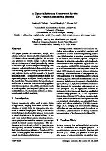
3. TEMPLATES FOR ETL ACTIVITIES.............................................................................................18 3.1 GENERAL FRAMEWORK .....................................................................................................................18 3.2 FORMAL DEFINITION AND USAGE OF TEMPLATE ACTIVITIES ............................................................20 3.2.1 Notation .....................................................................................................................................20 3.2.2 Instantiation...............................................................................................................................22 3.2.3 Taxonomy: Simple and Program-Based Templates...................................................................24 4. IMPLEMENTATION..........................................................................................................................27 5. RELATED WORK...............................................................................................................................30 5.1 COMMERCIAL STUDIES AND TOOLS ...................................................................................................30 5.2 RESEARCH EFFORTS ..........................................................................................................................31 5.3 APPLICATIONS OF ETL WORKFLOWS IN DATA WAREHOUSES. ...........................................................33 6. DISCUSSION .......................................................................................................................................34 7. CONCLUSIONS...................................................................................................................................36 REFERENCES .........................................................................................................................................37 APPENDIX ...............................................................................................................................................39

2

A GENERIC AND CUSTOMIZABLE FRAMEWORK FOR THE DESIGN OF ETL SCENARIOS PANOS VASSILIADIS1, ALKIS SIMITSIS2, PANOS GEORGANTAS2, MANOLIS TERROVITIS2, SPIROS SKIADOPOULOS2 1 University of Ioannina, Dept. of Computer Science, Ioannina, Greece [email protected]

2

National Technical University of Athens, Dept. of Electrical and Computer Eng., Athens, Greece {asimi, pgeor, mter, spiros}@dbnet.ece.ntua.gr

Abstract. Extraction-Transformation-Loading (ETL) tools are pieces of software responsible for the extraction of data from several sources, their cleansing, customization and insertion into a data warehouse. In this paper, we delve into the logical design of ETL scenarios and provide a generic and customizable framework in order to support the DW designer in his task. First, we present a metamodel particularly customized for the definition of ETL activities. We follow a workflow-like approach, where the output of a certain activity can either be stored persistently or passed to a subsequent activity. Also, we employ a declarative database programming language, LDL, to define the semantics of each activity. The metamodel is generic enough to capture any possible ETL activity. Nevertheless, in the pursuit of higher reusability and flexibility, we specialize the set of our generic metamodel constructs with a palette of frequently-used ETL activities, which we call templates. Moreover, in order to achieve a uniform extensibility mechanism for this library of built-ins, we have to deal with specific language issues. Therefore, we also discuss the mechanics of template instantiation to concrete activities. The design concepts that we introduce have been implemented in a tool, ARKTOS II, which is also presented. Keywords: Data warehousing, ETL

1. INTRODUCTION Data warehouse operational processes normally compose a labor intensive workflow, involving data extraction, transformation, integration, cleaning and transport. To deal with this workflow, specialized tools are already available in the market [IBM03,Info03,Micr02,Orac03], under the general title Extraction-Transformation-Loading (ETL) tools. To give a general idea of the functionality of these tools we mention their most prominent tasks, which include (a) the identification of relevant information at the source side, (b) the extraction of this information, (c) the customization and integration of the information coming from multiple sources into a common format, (d) the cleaning of the resulting data set, on the basis of database and business rules, and (e) the propagation of the data to the data warehouse and/or data marts. If we treat an ETL scenario as a composite workflow, in a traditional way, its designer is obliged to define several of its parameters (Fig. 1.1). Here, we follow a multi-perspective approach that enables to separate these parameters and study them in a principled approach. We are mainly interested in the design and administration parts of the lifecycle of the overall ETL process, and we depict them at the upper and lower part of Fig. 1.1, respectively. At the top of Fig. 1.1, we are mainly concerned with the static design artifacts for a workflow environment. We will follow a traditional approach and group the design artifacts into logical and physical, with each category comprising its own perspective. We depict the logical perspective on the left hand side of Fig. 1.1, and the physical perspective on the right hand side. At the logical perspective, we classify the design artifacts that give an abstract description of the workflow environment. First, the designer is responsible for defining an Execution Plan for the scenario. The definition of an execution plan can be seen from various perspectives. The Execution Sequence involves the specification of which activity runs first, second, and so on, which activities run in parallel, or when a semaphore is defined so that several activities are synchronized at a rendezvous point. ETL activities normally run in batch, so the designer needs to specify an Execution Schedule, i.e., the time points or events that trigger the execution of the scenario as a whole. Finally, due to system crashes, it is imperative that there exists a Recovery Plan, specifying the sequence of steps to be taken in the case of failure for a certain activity (e.g., retry to execute the activity, or undo any intermediate results produced so far). On the right-hand side of Fig. 1.1, we can also see the physical perspective, involving the registration of the actual entities that exist in the real world. We will reuse the terminology of [AHKB00] for the physical perspective. The Resource Layer comprises the definition of roles (human or software) that are responsible for executing the activities of the workflow. The Operational Layer, at the same time, comprises the software modules that implement the design entities of the logical perspective in the real

3

world. In other words, the activities defined at the logical layer (in an abstract way) are materialized and executed through the specific software modules of the physical perspective. At the lower part of Fig. 1.1, we are dealing with the tasks that concern the administration of the workflow environment and their dynamic behavior at runtime. First, an Administration Plan should be specified, involving the notification of the administrator either on-line (monitoring) or off-line (logging) for the status of an executed activity, as well as the security and authentication management for the ETL environment. Logical Perspective

Physical Perspective

Execution Plan Resource Layer

Execution Sequence Execution Schedule Recovery Plan Relationship with data

Operational Layer

Primary Data Flow Data Flow for Logical Exceptions

Administration Plan

Monitoring & Logging Security & Access Rights Management

Fig. 1.1 Different perspectives for an ETL workflow

We find that research has not dealt with the definition of data-centric workflows to the entirety of its extent. In the ETL case, for example, due to the data centric nature of the process, the designer must deal with the relationship of the involved activities with the underlying data. This involves the definition of a Primary Data Flow that describes the route of data from the sources towards their final destination in the data warehouse, as they pass through the activities of the scenario. Also, due to possible quality problems of the processed data, the designer is obliged to define a Data Flow for Logical Exceptions, i.e., a flow for the problematic data, i.e., the rows that violate integrity or business rules. It is the combination of the execution sequence and the data flow that generates the semantics of the ETL workflow: the data flow defines what each activity does and the execution plan defines in which order and combination. In this paper, we work in the internals of the data flow of ETL scenarios. First, we present a metamodel particularly customized for the definition of ETL activities. We follow a workflow-like approach, where the output of a certain activity can either be stored persistently or passed to a subsequent activity. Moreover, we employ a declarative database programming language, LDL, to define the semantics of each activity. The metamodel is generic enough to capture any possible ETL activity; nevertheless, reusability and ease-of-use dictate that we can do better in aiding the data warehouse designer in his task. In this pursuit of higher reusability and flexibility, we specialize the set of our generic metamodel constructs with a palette of frequently-used ETL activities, which we call templates. Moreover, in order to achieve a uniform extensibility mechanism for this library of built-ins, we have to deal with specific language issues: thus, we also discuss the mechanics of template instantiation to concrete activities. The design concepts that we introduce have been implemented in a tool, ARKTOS II, which is also presented. Our contributions can be listed as follows: - First, we define a formal metamodel as an abstraction of ETL processes at the logical level. The data stores, activities and their constituent parts are formally defined. An activity is defined as an entity

4

-

-

with possibly more than one input schemata, an output schema and a parameter schema, so that the activity is populated each time with its proper parameter values. The flow of data from producers towards their consumers is achieved through the usage of provider relationships that map the attributes of the former to the respective attributes of the latter. A serializable combination of ETL activities, provider relationships and data stores constitutes an ETL scenario. Second, we provide a reusability framework that complements the genericity of the metamodel. Practically, this is achieved from a set of “built-in” specializations of the entities of the Metamodel layer, specifically tailored for the most frequent elements of ETL scenarios. This palette of template activities will be referred to as Template layer and it is characterized by its extensibility; in fact, due to language considerations, we provide the details of the mechanism that instantiates templates to specific activities. Finally, we discuss implementation issues and we present a graphical tool, ARKTOS II that facilitates the design of ETL scenarios, based on our model.

This paper is organized as follows. In Section 2, we present a generic model of ETL activities. Section 3 describes the mechanism for specifying and materializing template definitions of frequently used ETL activities. Section 4 presents ARKTOS II, a prototype graphical tool. In Section 5, we present related work. In Section 6, we make a general discussion on the completeness and general applicability of our approach. Section 7 offers conclusions and presents topics for future research. Finally in the Appendix, we present a formal LDL description of the most frequently used ETL activities. Short versions of parts of this paper have been presented in [VaSS02, VSGT03].

5

2. GENERIC MODEL OF ETL ACTIVITIES The purpose of this section is to present a formal logical model for the activities of an ETL environment. This model abstracts from the technicalities of monitoring, scheduling and logging while it concentrates on the flow of data from the sources towards the data warehouse through the composition of activities and data stores. The full layout of an ETL scenario, involving activities, recordsets and functions can be modeled by a graph, which we call the Architecture Graph. We employ a uniform, graph-modeling framework for both the modeling of the internal structure of activities and for the modeling of the ETL scenario at large, which enables the treatment of the ETL environment from different viewpoints. First, the architecture graph comprises all the activities and data stores of a scenario, along with their components. Second, the architecture graph captures the data flow within the ETL environment. Finally, the information on the typing of the involved entities and the regulation of the execution of a scenario, through specific parameters are also covered. 2.1

Graphical Notation and Motivating Example

Being a graph, the Architecture Graph of an ETL scenario comprises nodes and edges. The involved data types, function types, constants, attributes, activities, recordsets, parameters and functions constitute the nodes of the graph. The different kinds of relationships among these entities are modeled as the edges of the graph. In Fig. 2.1, we give the graphical notation for all the modeling constructs that will be presented in the sequel. Data Types

Black ellipsis

Integer

Function Types

Black squares

$2€

Constants

Black cycles

1

Attributes

Hollow ellipsoid nodes

Part-Of Relationships

Simple edges annotated with diamond*

Provider Relationships

Instance-Of Relationships

Dotted arrows (from instance towards the type)

Derived Provider Relationships

Regulator Relationships

Dotted edges

* We annotate the part-of relationship among a function and its return type with a directed edge, to distinguish it from the rest of the parameters.

PKEY

RecordSets

Cylinders

Functions

Gray squares

my$2€

Parameters

White squares

rate

Activities

Triangles

R

SK

Bold solid arrows (from provider to consumer) Bold dotted arrows (from provider to consumer)

Fig. 2.1 Graphical notation for the Architecture Graph.

Motivating Example. To motivate our discussion we will present an example involving the propagation of data from a certain source S1, towards a data warehouse DW through intermediate recordsets. These recordsets belong to a Data Staging Area (DSA)1 DS. The scenario involves the propagation of data from the table PARTSUPP of source S1 to the data warehouse DW. Table DW.PARTSUPP(PKEY,SOURCE,DATE, QTY,COST) stores information for the available quantity (QTY) and cost (COST) of parts (PKEY) per source (SOURCE). The data source S1.PARTSUPP(PKEY,DATE,QTY,COST) records the supplies from a 1

In data warehousing terminology a DSA is an intermediate area of the data warehouse, specifically destined to enable the transformation, cleaning and integration of source data, before being loaded to the warehouse.

6

specific geographical region, e.g., Europe. All the attributes, except for the dates are instances of the Integer type. The scenario is graphically depicted in Fig. 2.2 and involves the following

transformations.

S1.PARTSUPP

FTP_PS1

DS.PS1_NEW.PKEY = DS.PS1_OLD.PKEY

COST

Diff_PS1

NotNull1

SOURCE = 1

DS.PS1_NEW

Source

DS.PS1

Add_Attr1

DS.PS1_OLD Diff_PS1 _REJ

NotNull1 _REJ

DS.PS1.PKEY LOOKUP.PKEY LOOKUP.SOURCE LOOKUP.SKEY

SK1

DW.PARTSUPP

Data Warehouse LOOKUP

DSA

Fig. 2.2 Bird’s-eye view of the motivating example

1. 2.

3.

4.

5.

2

First, we transfer via FTP_PS1 the snapshot from the source S1.PARTSUPP to the file DS.PS1_NEW of the DSA2. In the DSA we maintain locally a copy of the snapshot of the source as it was at the previous loading (we assume here the case of the incremental maintenance of the DW, instead of the case of the initial loading of the DW). The recordset DS.PS1_NEW(PKEY,DATE,QTY,COST) stands for the last transferred snapshot of S1.PARTSUPP. By detecting the difference of this snapshot with the respective version of the previous loading, DS.PS1_OLD(PKEY,DATE,QTY,COST), we can derive the newly inserted rows in S1.PARTSUPP. Note that the difference activity that we employ, namely Diff_PS1, checks for differences only on the primary key of the recordsets; thus, we ignore here any possible deletions or updates for the attributes COST, QTY of existing rows. Any not newly inserted row is rejected and so, it is propagated to Diff_PS1_REJ that stores all the rejected rows and its schema is identical to the input schema of the activity Diff_PS1. The rows that pass the activity Diff_PS1 are checked for null values of the attribute COST through the activity NotNull1. We store the rows whose COST is not NULL in the recordset DS.PS1(PKEY, DATE,QTY,COST). Rows having a NULL value for their COST are kept in the Diff_PS1_REJ recordset for further examination by the data warehouse administrator. Although we consider the data flow for only one source, S1, the data warehouse can clearly have more than one sources for part supplies. In order to keep track of the source of each row that enters in the DW, we need to add a ‘flag’ attribute, namely SOURCE, indicating 1 for the respective source. This is achieved through the activity Add_Attr1. Next, we assign a surrogate key on PKEY. In the data warehouse context, it is common tactics to replace the keys of the production systems with a uniform key, which we call a surrogate key [KRRT98]. The basic reasons for this kind of replacement are performance and semantic homogeneity. Textual attributes are not the best candidates for indexed keys and thus, need to be replaced by integer keys. At the same time, different production systems might use different keys for the same object, or the same key for different objects, resulting in the need for a global replacement of these values in the data warehouse. This replacement is performed through a lookup table of the form L(PRODKEY,SOURCE,SKEY). The SOURCE column is due to the fact that there can be synonyms in the different sources, which are mapped to different objects in the data warehouse. In our case, the activity that performs the surrogate key assignment for the attribute PKEY is SK1. It uses the lookup table LOOKUP(PKEY,SOURCE,SKEY). Finally, we populate the data warehouse with the output of the previous activity.

The technical points of the likes of FTP are mostly employed to show what kind of problems someone has to deal with in a practical situation, rather than to relate this kind of physical operations to a logical model. In terms of logical modelling this is a simple passing of data from one site to another.

7

The role of rejected rows depends on the peculiarities of each ETL scenario. If the designer needs to administrate these rows further, then he/she should use intermediate storage recordsets with the burden of an extra I/O cost. If the rejected rows should not have a special treatment, then the best solution is to be ignored; thus, in this case we avoid overload the scenario with any extra storage recordset. In our case, we annotate only two of the presented activities with a destination for rejected rows. Out of these, while NotNull1_REJ absolutely makes sense as a placeholder for problematic rows having non-acceptable NULL values, Diff_PS1_REJ is presented for demonstration reasons only. Finally, before proceeding, we would like to stress that we do not anticipate a manual construction of the graph by the designer; rather, we employ this section to clarify how the graph will look like once constructed. To assist a more automatic construction of ETL scenarios, we have implemented the ARKTOS II tool that supports the designing process through a friendly GUI. We present ARKTOS II in Section 4. 2.2

Preliminaries

In this subsection, we will introduce the formal modeling of data types, data stores and functions, before proceeding to the modeling of ETL activities. Elementary Entities. We assume the existence of a countable set of data types. Each data type T is characterized by a name and a domain, i.e., a countable set of values, called dom(T). The values of the domains are also referred to as constants. We also assume the existence of a countable set of attributes, which constitute the most elementary granules of the infrastructure of the information system. Attributes are characterized by their name and data type. The domain of an attribute is a subset of the domain of its data type. Attributes and constants are uniformly referred to as terms. A Schema is a finite list of attributes. Each entity that is characterized by one or more schemata will be called Structured Entity. Moreover, we assume the existence of a special family of schemata, all under the general name of NULL Schema, determined to act as placeholders for data which are not to be stored permanently in some data store. We refer to a family instead of a single NULL schema, due to a subtle technicality involving the number of attributes of such a schema (this will become clear in the sequel). RecordSets. We define a record as the instantiation of a schema to a list of values belonging to the domains of the respective schema attributes. We can treat any data structure as a record set provided that there are the means to logically restructure it into a flat, typed record schema. Several physical storage structures abide by this rule, such as relational databases, COBOL or simple ASCII files, multidimensional cubes, etc. We will employ the general term Recordset in order to refer to this kind of structures. For example, the schema of multidimensional cubes is of the form [D1,...,Dn,M1,...,Mm] where the Di represent dimensions (forming the primary key of the cube) and the Mj measures [VaSk00]. COBOL files, as another example, are records with fields having two peculiarities: nested records and alternative representations. One can easily unfold the nested records and choose one of the alternative representations. Relational databases are clearly recordsets, too. Formally, a recordset is characterized by its name, its (logical) schema and its (physical) extension (i.e., a finite set of records under the recordset schema). If we consider a schema S=[A1,…,Ak], for a certain recordset, its extension is a mapping S=[A1,…,Ak]→dom(A1)×…×dom(Ak). Thus, the extension of the recordset is a finite subset of dom(A1)×…×dom(Ak) and a record is the instance of a mapping dom(A1)×…×dom(Ak)→[x1,…,xk], xi∈dom(Ai). In the rest of this paper we will mainly deal with the two most popular types of recordsets, namely relational tables and record files. A database is a finite set of relational tables. Functions. We assume the existence of a countable set of built-in system function types. A function type comprises a name, a finite list of parameter data types, and a single return data type. A function is an instance of a function type. Consequently, it is characterized by a name, a list of input parameters and a parameter for its return value. The data types of the parameters of the generating function type define also (a) the data types of the parameters of the function, and (b) the legal candidates for the function parameters (i.e., attributes or constants of a suitable data type).

8

2.3

Activities

Activities are the backbone of the structure of any information system. We adopt the WfMC terminology [WfMC98] for processes/programs and we will call them activities in the sequel. An activity is an amount of “work which is processed by a combination of resource and computer applications” [WfMC98]. In our framework, activities are logical abstractions representing parts, or full modules of code. The execution of an activity is performed from a particular program. Normally, ETL activities will be either performed in a black-box manner by a dedicated tool, or they will be expressed in some language (e.g., PL/SQL, Perl, C). Still, we want to deal with the general case of ETL activities. We employ an abstraction of the source code of an activity, in the form of an LDL statement. Using LDL we avoid dealing with the peculiarities of a particular programming language. Once again, we want to stress that the presented LDL description is intended to capture the semantics of each activity, instead of the way these activities are actually implemented. An Elementary Activity is formally described by the following elements: - Name: a unique identifier for the activity. - Input Schemata: a finite set of one or more input schemata that receive data from the data providers of the activity. - Output Schema: a schema that describes the placeholder for the rows that pass the check performed by the elementary activity. - Rejections Schema: a schema that describes the placeholder for the rows that do not pass the check performed by the activity, or their values are not appropriate for the performed transformation. - Parameter List: a set of pairs which act as regulators for the functionality of the activity (the target attribute of a foreign key check, for example). The first component of the pair is a name and the second is a schema, an attribute, a function or a constant. - Output Operational Semantics: an LDL statement describing the content passed to the output of the operation, with respect to its input. This LDL statement defines (a) the operation performed on the rows that pass through the activity and (b) an implicit mapping between the attributes of the input schema(ta) and the respective attributes of the output schema. - Rejection Operational Semantics: an LDL statement describing the rejected records, in a sense similar to the Output Operational Semantics. This statement is by default considered to be the complement of the Output Operational Semantics, except if explicitly defined differently. There are two issues that we would like to elaborate on, here: - NULL Schemata. Whenever we do not specify a data consumer for the output or rejection schemata, the respective NULL schema (involving the correct number of attributes) is implied. This practically means that the data targeted for this schema will neither be stored to some persistent data store, nor will they be propagated to another activity, but they will simply be ignored. - Language Issues. Initially, we used to specify the semantics of activities with SQL statements. Still, although clear and easy to write and understand, SQL is rather hard to use if one is to perform rewriting and composition of statements. Thus, we have supplemented SQL with LDL [NaTs98], a logic-programming, declarative language as the basis of our scenario definition. LDL is a Datalog variant based on a Horn-clause logic that supports recursion, complex objects and negation. In the context of its implementation in an actual deductive database management system, LDL++ [Zani98], the language has been extended to support external functions, choice, aggregation (and even, userdefined aggregation), updates and several other features. 2.4

Relationships in the Architecture Graph

In this subsection, we will elaborate on the different kinds of relationships that the entities of an ETL scenario have. Whereas these entities are modeled as the nodes of the architecture graph, the relationships are modeled as its edges. Due to their diversity, before proceeding, we list these types of relationships along with the related terminology that we will employ for the rest of the paper. The graphical notation of entities (nodes) and relationships (edges) is presented in Fig. 2.1. - Part-of relationships. These relationships involve attributes and parameters and relate them to the respective activity, recordset or function to which they belong. - Instance-of relationships. These relationships are defined among a data/function type and its instances.

9

-

Provider relationships. These are relationships that involve attributes with a provider-consumer relationship. Regulator relationships. These relationships are defined among the parameters of activities and the terms that populate these activities. Derived provider relationships. A special case of provider relationships that occurs whenever output attributes are computed through the composition of input attributes and parameters. Derived provider relationships can be deduced from a simple rule and do not originally constitute a part of the graph.

In the rest of this subsection, we will base our discussions on a part of the scenario of the motivating example (presented in Section 2.1), including the activities Add_Attr1 and SK1. DS.PS1

OUT

IN

Add_Attr1

OUT

IN

PAR

OUT

SK1

IN

PAR

PKEY

PKEY

PKEY

PKEY

PKEY

PKEY

QTY

QTY

QTY

QTY

QTY

QTY

COST

COST

COST

COST

COST

COST

DATE

DATE

DATE

DATE

DATE

DATE

SOURCE

SOURCE

SOURCE

SOURCE

SKEY

AddConst1

in

DW.PARTS UPP

PKEY

out

SOURCE 1

LOOKUP

OUT

PKEY

LPKEY

SOURCE

LSOURCE

SKEY

LSKEY

Fig. 2.3 Part-of relationships of the architecture graph

Attributes and part-of relationships. The first thing to incorporate in the architecture graph is the structured entities (activities and recordsets) along with all the attributes of their schemata. We choose to avoid overloading the notation by incorporating the schemata per se; instead we apply a direct part-of relationship between an activity node and the respective attributes. We annotate each such relationship with the name of the schema (by default, we assume a IN, OUT, PAR, REJ tag to denote whether the attribute belongs to the input, output, parameter or rejection schema of the activity respectively). Naturally, if the activity involves more than one input schemata, the relationship is tagged with an INi tag for the ith input schema. We also incorporate the functions along with their respective parameters and the part-of relationships among the former and the latter. We annotate the part-of relationship with the return type with a directed edge, to distinguish it from the rest of the parameters. Fig. 2.3 depicts a part of the motivating example, where we can see the decomposition of (a) the recordsets DS.PS1, LOOKUP, DW.PARTSUPP; (b) the activities Add_Attr1 and SK1 into the attributes of their input and output schemata. Note the tagging of the schemata of the involved activities. We do not consider the rejection schemata in order to avoid crowding the picture. At the same time, the function AddConst1 is decomposed into its parameters. This function belongs to the function type ADD_CONST and comprises two parameters: in and out. The former receives an integer as input and the latter returns this integer. As we will see in the sequel, this value will be propagated towards the SOURCE attribute, in order to trace the fact that the propagated rows come from source S1. Note also, how the parameters of the two activities are also incorporated in the architecture graph. For the case of activity Add_Attr1 the involved parameters are the parameters in and out of the employed function. For the case of activity SK1 we have five parameters: (a) PKEY, which stands for the production key to be replaced; (b) SOURCE, which stands for an integer value that characterizes which source’s data

10

are processed; (c) LPKEY, which stands for the attribute of the lookup table which contains the production keys; (d) LSOURCE, which stands for the attribute of the lookup table which contains the source value (corresponding to the aforementioned SOURCE parameter); (e) LSKEY, which stands for the attribute of the lookup table which contains the surrogate keys. DS.PS1

OUT

IN

Add_Attr1

OUT

IN

OUT

SK1

IN

DW.PARTS UPP

PAR

Date

Integer

PKEY

PKEY

PKEY

PKEY

PKEY

PKEY

QTY

QTY

QTY

QTY

QTY

QTY

COST

COST

COST

COST

COST

COST

DATE

DATE

DATE

DATE

DATE

DATE

SOURCE

SOURCE

SOURCE

SOURCE

ADD_CONST

SKEY

AddConst1

Fig. 2.4 Instance-of relationships of the architecture graph

Data types and instance-of relationships. To capture typing information on attributes and functions, the architecture graph comprises data and function types. Instantiation relationships are depicted as dotted arrows that stem from the instances and head towards the data/function types. In Fig. 2.4, we observe the attributes of the two activities of our example and their correspondence to two data types, namely Integer and Date. For reasons of presentation, we merge several instantiation edges so that the figure does not become too crowded. At the bottom of Fig. 2.4, we can also see the fact that function AddConst1 is an instance of the function type ADD_CONST. Parameters and regulator relationships. Once the part-of and instantiation relationships have been established, it is time to establish the regulator relationships of the scenario. In this case, we link the parameters of the activities to the terms (attributes or constants) that populate them. We depict regulator relationships with simple dotted edges. DS.PS1

OUT

IN

Add_Attr1

OUT

IN

PAR

OUT

SK1

IN

PAR

PKEY

PKEY

PKEY

PKEY

PKEY

PKEY

QTY

QTY

QTY

QTY

QTY

QTY

COST

COST

COST

COST

COST

COST

DATE

DATE

DATE

DATE

DATE

DATE

SOURCE

SOURCE

SOURCE

SOURCE

SKEY

AddConst1

in

DW.PARTS UPP

PKEY

out

SOURCE 1

LOOKUP

OUT

PKEY

LPKEY

SOURCE

LSOURCE

SKEY

LSKEY

Fig. 2.5 Regulator relationships of the architecture graph

In the example of Fig. 2.5 we can observe how the parameters of the two activities are populated. First, we can see that activity Add_Attr1 receives an integer (1) as its input and uses the function AddConst1

11

to populate its attribute SOURCE. The parameters in and out are mapped to the respective terms through regulator relationships. The same applies also for activity SK1. All its parameters, namely PKEY, SOURCE, LPKEY, LSOURCE and LSKEY, are mapped to the respective attributes of either the activity’s input schema or the employed lookup table LOOKUP. The parameter LSKEY deserves particular attention. This parameter is (a) populated from the attribute SKEY of the lookup table and (b) used to populate the attribute SKEY of the output schema of the activity. Thus, two regulator relationships are related with parameter LSKEY, one for each of the aforementioned attributes. The existence of a regulator relationship among a parameter and an output attribute of an activity normally denotes that some external data provider is employed in order to derive a new attribute, through the respective parameter. Provider relationships. The flow of data from the data sources towards the data warehouse is performed through the composition of activities in a larger scenario. In this context, the input for an activity can be either a persistent data store, or another activity, i.e., any structured entity under a specific schema. Usually, this applies for the output of an activity, too. We capture the passing of data from providers to consumers by a Provider Relationship among the attributes of the involved schemata. Formally, a Provider Relationship is defined as follows: - Name: a unique identifier for the provider relationship. - Mapping: an ordered pair. The first part of the pair is a term (i.e., an attribute or constant), acting as a provider and the second part is an attribute acting as the consumer. The mapping need not necessarily be 1:1 from provider to consumer attributes, since an input attribute can be mapped to more than one consumer attributes. Still, the opposite does not hold. Note that a consumer attribute can also be populated by a constant, in certain cases. In order to achieve the flow of data from the providers of an activity towards its consumers, we need the following three groups of provider relationships: 1. A mapping between the input schemata of the activity and the output schema of their data providers. In other words, for each attribute of an input schema of an activity, there must exists an attribute of the data provider, or a constant, which is mapped to the former attribute. 2. A mapping between the attributes of the activity input schemata and the activity output (or rejection, respectively) schema. 3. A mapping between the output or rejection schema of the activity and the (input) schema of its data consumer. The mappings of the second type are internal to the activity. Basically, they can be derived from the LDL statement for each of the output/rejection schemata. As far as the first and the third types of provider relationships are concerned, the mappings must be provided during the construction of the ETL scenario. This means that they are either (a) by default assumed by the order of the attributes of the involved schemata or (b) hard-coded by the user. Provider relationships are depicted with bold solid arrows that stem from the provider and end in the consumer attribute. Observe Fig. 2.6. The flow starts from table DS.PS1 of the data staging area. Each of the attributes of this table is mapped to an attribute of the input schema of activity Add_Attr1. The attributes of the input schema of the latter are subsequently mapped to the attributes of the output schema of the activity. The flow continues from activity Add_Attr1 towards the activity SK1 in a similar manner. Note that, for the moment, we have not covered how the output of function AddConst1 populates the output attribute SOURCE for the activity Add_Attr1, or how the parameters of activity SK1 populate the output attribute SKEY. Such information will be expressed using derived provider relationships, which we will introduce in the sequel. Another interesting thing is that during the data flow, new attributes are generated, resulting on new streams of data, whereas the flow seems to stop for other attributes. Observe the rightmost part of Fig. 2.6 where the values of attribute PKEY are not further propagated (remember that the reason for the application of a surrogate key transformation is to replace the production keys of the source data to a homogeneous surrogate for the records of the data warehouse, which is independent of the source they have been collected from). Instead of the values of the production key, the values from the attribute SKEY will be used to denote the unique identifier for a part in the rest of the flow.

12

DS.PS1

OUT

IN

Add_Attr1

OUT

IN

PAR

OUT

SK1

IN

PAR

PKEY

PKEY

PKEY

PKEY

PKEY

PKEY

QTY

QTY

QTY

QTY

QTY

QTY

COST

COST

COST

COST

COST

COST

DATE

DATE

DATE

DATE

DATE

DATE

SOURCE

SOURCE

SOURCE

SOURCE

SKEY

AddConst1

in

DW.PARTS UPP

PKEY

out

SOURCE 1

LOOKUP

OUT

PKEY

LPKEY

SOURCE

LSOURCE

SKEY

LSKEY

Fig. 2.6 Provider relationships of the architecture graph

Derived provider relationships. As we have already mentioned, there are certain output attributes that are computed through the composition of input attributes and parameters. A derived provider relationship is another form of provider relationship that captures the flow from the input to the respective output attributes. Formally, assume that source is a term in the architecture graph, target is an attribute of the output schema of an activity A and x,y are parameters in the parameter list of A. It is not necessary that the parameters x and y be different with each other. Then, a derived provider relationship pr(source, target) exists iff the following regulator relationships (i.e., edges) exist: rr1(source,x) and rr2(y,target). Intuitively, the case of derived relationships models the situation where the activity computes a new attribute in its output. In this case, the produced output depends on all the attributes that populate the parameters of the activity, resulting in the definition of the corresponding derived relationship. Observe Fig. 2.7, where we depict a small part of our running example. The legend in the left side of Fig. 2.7 depicts how the attributes that populate the parameters of the activity are related through derived provider relationships with the computed output attribute SKEY. The meaning of these five relationships is that SK1.OUT.SKEY is not computed only from attribute LOOKUP.SKEY, but from the combination of all the attributes that populate the parameters. As far as the parameters of activity Add_Attr1 are concerned, we can also detect a derived provider relationship, between the constant 1 and the output attribute SOURCE. Again, in this case, the constant is the only term that applies for the parameters of the activity and the output attribute is linked to the parameter schema through a regulator relationship. One can also assume different variations of derived provider relationships such as (a) relationships that do not involve constants (remember that we have defined source as a term); (b) relationships involving only attributes of the same/different activity (as a measure of internal complexity or external dependencies); (c) relationships relating attributes that populate only the same parameter (e.g., only the attributes LOOKUP.SKEY and SK1.OUT.SKEY).

13

Fig. 2.7 Derived provider relationships of the architecture graph

2.5

Scenarios

A Scenario is an enumeration of activities along with their source/target recordsets and the respective provider relationships for each activity. Formally, a Scenario consists of: - Name: a unique identifier for the scenario. - Activities: A finite list of activities. Note that by employing a list (instead of e.g., a set) of activities, we impose a total ordering on the execution of the scenario. - Recordsets: A finite set of recordsets. - Targets: A special-purpose subset of the recordsets of the scenario, which includes the final destinations of the overall process (i.e., the data warehouse tables that must be populated by the activities of the scenario). - Provider Relationships: A finite list of provider relationships among activities and recordsets of the scenario. Intuitively, a scenario is a set of activities, deployed along a graph in an execution sequence that can be linearly serialized. For the moment, we do not consider the different alternatives for the ordering of the execution; we simply require that a total order for this execution is present (i.e., each activity has a discrete execution priority). In general, there is a simple rule for constructing valid ETL scenarios in our setting. For each activity, the designer must provide three kinds of provider relationships: (a) a mapping of the activity's data provider(s) to the activity's input schema(ta); (b) a mapping of the activity's input schema(ta) to the activity's output, along with a specification of the semantics of the activity (i.e., the check / cleaning / transformation / value production that the activity performs), and (c) a mapping from the activity's output schema towards the data consumer of the activity. Moreover, we assume the following Integrity Constraints for a scenario: Static Constraints: - All the weak entities of a scenario (i.e., attributes or parameters) should be defined within a part-of relationship (i.e., they should have a container object). - All the mappings in provider relationships should be defined among terms (i.e., attributes or constants) of the same data type. Data Flow Constraints: - All the attributes of the input schema(ta) of an activity should have a provider.

14

-

Resulting from the previous requirement, if some attribute is a parameter in an activity A, the container of the attribute (i.e., recordset or activity) should precede A in the scenario. All the attributes of the schemata of the target recordsets should have a data provider.

In terms of formal modeling of the architecture graph, we assume the infinitely countable, mutually disjoint sets of names (i.e., the values of which respect the unique name assumption) of column Modelspecific in Fig. 2.8. As far as a specific scenario is concerned, we assume their respective finite subsets, depicted in column Scenario-Specific in Fig. 2.8. Data types, function types and constants are considered Built-in’s of the system, whereas the rest of the entities are provided by the user (User Provided).

User-provided

Built -in

Entity Data Types Function Types Constants Attributes Functions Schemata RecordSets Activities Provider Relationships Part-Of Relationships Instance-Of Relationships Regulator Relationships Derived Provider Relationships

Model-specific

Scenario-specific

DI FI CI ΩI ΦI SI RSI AI PrI PoI IoI RrI DrI

D F C Ω Φ S RS A Pr Po Io Rr Dr

Fig. 2.8 Formal definition of domains and notation

Formally, let G(V,E) be the Architecture Graph of an ETL scenario. Then, V = D∪F∪C∪Ω∪Φ∪S∪RS∪A E = Pr∪Po∪Io∪Rr∪Dr 2.6

Motivating Example Revisited

In this subsection, we return to our motivating example, in order (a) to summarize how it is modeled in terms of our architecture graph, from different viewpoints and (b) to show how its declarative description in LDL looks like. Fig. 2.9 depicts a screenshot of ARKTOS II that represents a zoom-in of the last two activities of the scenario. We can observe (from right to left): (i) the fact that the recordset DW.PARTSUPP comprises the attributes PKEY,SOURCE,DATE,QTY,COST (ii) the provider relationships (bold and solid arrows) between the output schema of the activity SK1 and the attributes of DW.PARTSUPP; (iii) the provider relationships between the input and the output schema of activity SK1; (iv) the provider relationships between the output schema of the activity Add_Attr1 and the input schema of the activity SK1; (v) the population of the parameters of the surrogate key activity from regulator relationships (dotted bold arrows) by the attributes of table LOOKUP and some of the attribute of the input schema of SK1; (vi) the instance-of relationships (light dotted edges) between the attributes of the scenario and their data types (colored ovals at the bottom of the figure).

15

Fig. 2.9 Architecture graph of a part of the motivating example

In Fig. 2.10, we show the LDL program for our motivating example. In the next section, we will also elaborate in adequate detail on the mechanics of the usage of LDL for ETL scenarios. diffPS1_in1(A_IN1_PKEY,A_IN1_DATE,A_IN1_QTY,A_IN1_COST) Å ds_ps1_new(A_IN1_PKEY,A_IN1_DATE,A_IN1_QTY,A_IN1_COST). diffPS1_in2(A_IN1_PKEY,A_IN1_DATE,A_IN1_QTY,A_IN1_COST Å ds_ps1_old(A_IN1_PKEY,A_IN1_DATE,A_IN1_QTY,A_IN1_COST). semi_join(A_OUT_PKEY,A_OUT_DATE,A_OUT_QTY,A_OUT_COST) Å diffPS1_in1(A_IN1_PKEY,A_IN1_DATE,A_IN1_QTY,A_IN1_COST), diffPS1_in2(A_IN2_PKEY,_,_,_), A_OUT_PKEY=A_IN1_PKEY, A_OUT_PKEY=A_IN2_PKEY, A_OUT_DATE=A_IN1_DATE, A_OUT_QTY=A_IN1_QTY, A_OUT_COST=A_IN1_COST. diffPS1_out(A_OUT_PKEY,A_OUT_DATE,A_OUT_QTY,A_OUT_COST) Å diffPS1_in1(A_IN1_PKEY,A_IN1_DATE,A_IN1_QTY,A_IN1_COST), ~semi_join(A_IN1_PKEY,A_IN1_DATE,A_IN1_QTY,A_IN1_COST), A_OUT_PKEY=A_IN1_PKEY, A_OUT_DATE=A_IN1_DATE, A_OUT_QTY=A_IN1_QTY, A_OUT_COST=A_IN1_COST. diffPS1_rej(A_REJ_PKEY,A_REJ_DATE,A_REJ_QTY,A_REJ_COST) Å diffPS1_in1(A_IN1_PKEY,A_IN1_DATE,A_IN1_QTY,A_IN1_COST), semi_join(A_IN1_PKEY,A_IN1_DATE,A_IN1_QTY,A_IN1_COST), A_REJ_PKEY=A_IN1_PKEY, A_REJ_DATE=A_IN1_DATE, A_REJ_QTY=A_IN1_QTY, A_REJ_COST=A_IN1_COST. diff_PS1_REJ Å (A_REJ_PKEY,A_REJ_DATE,A_REJ_QTY,A_REJ_COST) diffPS1_rej (A_REJ_PKEY,A_REJ_DATE,A_REJ_QTY,A_REJ_COST) notNull_in1(A_IN1_ PKEY,A_IN1_DATE,A_IN1_QTY,A_IN1_COST) Å diff_PS1_out(A_OUT_PKEY,A_OUT_DATE,A_OUT_QTY,A_OUT_COST), A_OUT_PKEY=A_IN1_PKEY, A_OUT_DATE=A_IN1_DATE, A_OUT_QTY=A_IN1_QTY, A_OUT_COST=A_IN1_COST. notNull_out(A_OUT_PKEY,A_OUT_DATE,A_OUT_QTY,A_OUT_COST) Å notNull_in1(A_IN1_PKEY,A_IN1_DATE,A_IN1_QTY,A_IN1_COST),

16

A_IN1_COST~=’null’, A_OUT_PKEY=A_IN1_PKEY, A_OUT_DATE=A_IN1_DATE, A_OUT_QTY=A_IN1_QTY, A_OUT_COST=A_IN1_COST. notNull_rej(A_REJ_PKEY,A_REJ_DATE,A_REJ_QTY,A_REJ_COST) Å notNull_in1(A_IN1_PKEY,A_IN1_DATE,A_IN1_QTY,A_IN1_COST), A_IN1_COST=’null’, A_REJ_PKEY=A_IN1_PKEY, A_REJ_DATE=A_IN1_DATE, A_REJ_QTY=A_IN1_QTY, A_REJ_COST=A_IN1_COST. not_Null_REJ(A_REJ_PKEY,A_REJ_DATE,A_REJ_QTY,A_REJ_COST) Å notNull_rej(A_REJ_PKEY,A_REJ_DATE,A_REJ_QTY,A_REJ_COST). ds_ps1(PKEY,DATE,QTY,COST) Å a_out(A_OUT_PKEY,A_OUT_DATE,A_OUT_QTY,A_OUT_COST), PKEY=A_OUT_PKEY, DATE=A_OUT_DATE, QTY=A_OUT_QTY, COST=A_OUT_COST. addAttr_in1(A_IN1_PKEY,A_IN1_DATE,A_IN1_QTY,A_IN1_COST) Å ds_ps1(PKEY,DATE,QTY,COST), PKEY=A_IN1_PKEY, DATE=A_IN1_DATE, QTY=A_IN1_QTY, COST=A_IN1_COST. addAttr_out(A_OUT_PKEY,A_OUT_DATE,A_OUT_QTY,A_OUT_COST,A_OUT_SOURCE) Å addAttr_in1(A_IN1_PKEY,A_IN1_DATE,A_IN1_QTY,A_IN1_COST), A_OUT_PKEY=A_IN1_PKEY, A_OUT_DATE=A_IN1_DATE, A_OUT_QTY=A_IN1_QTY, A_OUT_COST=A_IN1_COST, A_OUT_SOURCE='SOURCE1'. addSkey_in1(A_IN1_PKEY,A_IN1_DATE,A_IN1_QTY,A_IN1_COST,A_IN1_SOURCE) Å addAttr_out(A_OUT_PKEY,A_OUT_DATE,A_OUT_QTY,A_OUT_COST,A_OUT_SOURCE), A_OUT_PKEY=A_IN1_PKEY, A_OUT_DATE=A_IN1_DATE, A_OUT_QTY=A_IN1_QTY, A_OUT_COST=A_IN1_COST, A_OUT_SOURCE=A_IN1_SOURCE. addSkey_out(A_OUT_PKEY,A_OUT_DATE,A_OUT_QTY,A_OUT_COST,A_OUT_SOURCE,A_OUT_SKEY) Å addSkey_in1(A_IN1_PKEY,A_IN1_DATE,A_IN1_QTY,A_IN1_COST,A_IN1_SOURCE), lookup(A_IN1_SOURCE,A_IN1_PKEY,A_OUT_SKEY), A_OUT_PKEY=A_IN1_PKEY, A_OUT_DATE=A_IN1_DATE, A_OUT_QTY=A_IN1_QTY, A_OUT_COST=A_IN1_COST, A_OUT_SOURCE=A_IN1_SOURCE. dw_partsupp(PKEY,DATE,QTY,COST,SOURCE) Å addSkey_out(A_OUT_PKEY,A_OUT_DATE,A_OUT_QTY,A_OUT_COST,A_OUT_SOURCE,A_OUT_SKEY), DATE=A_IN1_DATE, QTY=A_IN1_QTY, COST=A_IN1_COST SOURCE=A_IN1_SOURCE, PKEY=A_IN1_SKEY. NOTE: For reasons of readability we de not replace the ’A’ in attribute names with the activity name, i.e., A_OUT_PKEY should be diffPS1_OUT_PKEY.

Fig. 2.10 LDL specification of the motivating example

17

3. TEMPLATES FOR ETL ACTIVITIES In this section, we present the mechanism for exploiting template definitions of frequently used ETL activities. The general framework for the exploitation of these templates is accompanied with the presentation of the language-related issues for template management and appropriate examples. 3.1 General Framework Our philosophy during the construction of our metamodel was based on two pillars: (a) genericity, i.e., the derivation of a simple model, powerful to capture ideally all the cases of ETL activities and (b) extensibility, i.e., the possibility of extending the built-in functionality of the system with new, userspecific templates. The genericity doctrine was pursued through the definition of a rather simple activity metamodel, as described in Section 2. Still, providing a single metaclass for all the possible activities of an ETL environment is not really enough for the designer of the overall process. A richer “language” should be available, in order to describe the structure of the process and facilitate its construction. To this end, we provide a palette of template activities, which are specializations of the generic metamodel class. Observe Fig. 3.1 for a further explanation of our framework. The lower layer of Fig. 3.1, namely Schema Layer, involves a specific ETL scenario. All the entities of the Schema layer are instances of the classes Data Type, Function Type, Elementary Activity, RecordSet and Relationship. Thus, as one can see on the upper part of Fig. 3.1, we introduce a meta-class layer, namely Metamodel Layer involving the aforementioned classes. The linkage between the Metamodel and the Schema layers is achieved through instantiation (InstanceOf) relationships. The Metamodel layer implements the aforementioned genericity desideratum: the classes which are involved in the Metamodel layer are generic enough to model any ETL scenario, through the appropriate instantiation.

Fig. 3.1 The metamodel for the logical entities of the ETL environment

Still, we can do better than the simple provision of a meta- and an instance layer. In order to make our metamodel truly useful for practical cases of ETL activities, we enrich it with a set of ETL-specific constructs, which constitute a subset of the larger Metamodel layer, namely the Template Layer. The constructs in the Template layer are also meta-classes, but they are quite customized for the regular cases of ETL activities. Thus, the classes of the Template layer are specializations (i.e., subclasses) of the generic classes of the Metamodel layer (depicted as IsA relationships in Fig. 3.1). Through this customization mechanism, the designer can pick the instances of the Schema layer from a much richer palette of constructs; in this setting, the entities of the Schema layer are instantiations, not only of the respective classes of the Metamodel layer, but also of their subclasses in the Template layer.

18

In the example of Fig. 3.1 the concept DW.PARTSUPP must be populated from a certain source S1.PARTSUPP. Several operations must intervene during the propagation: for example, checks for null values and domain violations, as well as a surrogate key assignment take place in the scenario. As one can observe, the recordsets that take part in this scenario are instances of class RecordSet (belonging to the Metamodel layer) and specifically of its subclasses Source Table and Fact Table. Instances and encompassing classes are related through links of type InstanceOf. The same mechanism applies to all the activities of the scenario, which are (a) instances of class Elementary Activity and (b) instances of one of its subclasses, depicted in Fig. 3.1. Relationships do not escape the rule either: observe how the provider links from the concept S1.PS towards the concept DW.PARTSUPP are related to class Provider Relationship through the appropriate InstanceOf links. As far as the class Recordset is concerned, in the Template layer we can specialize it to several subclasses, based on orthogonal characteristics, such as whether it is a file or RDBMS table, or whether it is a source or target data store (as in Fig. 3.1). In the case of the class Relationship, there is a clear specialization in terms of the five classes of relationships which have already been mentioned in Section 2: Provider, Part-Of, Instance-Of, Regulator and Derived Provider. Following the same framework, class Elementary Activity is further specialized to an extensible set of reoccurring patterns of ETL activities, depicted in Fig. 3.2. As one can see on the top side of Fig. 3.1, we group the template activities in five major logical groups. We do not depict the grouping of activities in subclasses in Fig. 3.1, in order to avoid overloading the figure; instead, we depict the specialization of class Elementary Activity to three of its subclasses whose instances appear in the employed scenario of the Schema layer. We now proceed to present each of the aforementioned groups in more detail. Filters

Unary operations

Binary operations

- Selection (σ) - Not null (NN) - Primary key violation (PK) - Foreign key violation (FK) - Unique value (UN) - Domain mismatch (DM)

-

-

Push Aggregation (γ) Projection (π) Function application (f) Surrogate key assignment (SK) Tuple normalization (N) Tuple denormalization (DN)

Union (U) Join (>< ) Diff (∆) Update Detection (∆UPD)

File operations

Transfer operations

- EBCDIC to ASCII conversion (EB2AS) Sort file (Sort)

- Ftp (FTP) - Compress/Decompress (Z/dZ) Encrypt/Decrypt (Cr/dCr)

Fig. 3.1 Template activities, along with their graphical notation symbols, grouped by category

The first group, named Filters, provides checks for the satisfaction (or not) of a certain condition. The semantics of these filters are the obvious (starting from a generic selection condition and proceeding to the check for null values, primary or foreign key violation, etc.). The second group of template activities is called Unary Operations and except for the most generic push activity (which simply propagates data from the provider to the consumer), consists of the classical aggregation and function application operations along with three data warehouse specific transformations (surrogate key assignment, normalization and denormalization). The third group consists of classical Binary Operations, such as union, join and difference of recordsets/activities as well as with a special case of difference involving the detection of updates. Except for the aforementioned template activities, which mainly refer to logical transformations, we can also consider the case of physical operators that refer to the application of physical transformations to whole files/tables. In the ETL context, we are mainly interested in operations like Transfer Operations (ftp, compress/ decompress, encrypt/decrypt) and File Operations (EBCDIC to ASCII, sort file). Summarizing, the Metamodel layer is a set of generic entities, able to represent any ETL scenario. At the same time, the genericity of the Metamodel layer is complemented with the extensibility of the Template layer, which is a set of “built-in” specializations of the entities of the Metamodel layer, specifically tailored for the most frequent elements of ETL scenarios. Moreover, apart from this “built-in”, ETLspecific extension of the generic metamodel, if the designer decides that several ‘patterns’, not included in the palette of the Template layer, occur repeatedly in his data warehousing projects, he can easily fit them into the customizable Template layer through a specialization mechanism.

19

3.2 Formal Definition and Usage of Template Activities Once the template layer has been introduced, the obvious issue that is raised is its linkage with the employed declarative language of our framework. In general, the broader issue is the usage of the template mechanism from the user; to this end, we will explain the substitution mechanism for templates in this subsection and refer the interested reader to Appendix A for a presentation of the specific templates that we have constructed. A Template Activity is formally defined as follows: - Name: a unique identifier for the template activity. - Parameter List: a set of names which act as regulators in the expression of the semantics of the template activity. For example, the parameters are used to assign values to constants, create dynamic mapping at instantiation time, etc. - Expression: a declarative statement describing the operation performed by the instances of the template activity. As with elementary activities, our model supports LDL as the formalism for the expression of this statement. - Mapping: a set of bindings, mapping input to output attributes, possibly through intermediate placeholders. In general, mappings at the template level try to capture a default way of propagating incoming values from the input towards the output schema. These default bindings are easily refined and possibly rearranged at instantiation time. The template mechanism we use is a substitution mechanism, based on macros, that facilitates the automatic creation of LDL code. This simple notation and instantiation mechanism permits the easy and fast registration of LDL templates. In the rest of this section, we will elaborate on the notation, instantiation mechanisms and template taxonomy particularities. 3.2.1 Notation Our template notation is a simple language featuring five main mechanisms for dynamic production of LDL expressions: (a) variables that are replaced by their values at instantiation time; (b) a function that returns the arity of an input, output or parameter schema; (c) loops, where the loop body is repeated at instantiation time as many times as the iterator constraint defines; (d) keywords to simplify the creation of unique predicate and attribute names; and, finally, (e) macros which are used as syntactic sugar to simplify the way we handle complex expressions (especially in the case of variable size schemata). Variables. We have two kinds of variables in the template mechanism: parameter variables and loop iterators. Parameter variables are marked with a @ symbol at their beginning and they are replaced by user-defined values at instantiation time. A list of an arbitrary length of parameters is denoted by @[]. For such lists the user has to explicitly or implicitly provide their length at instantiation time. Loop iterators, on the other hand, are implicitly defined in the loop constraint. During each loop iteration, all the properly marked appearances of the iterator in the loop body are replaced by its current value (similarly to the way the C preprocessor treats #DEFINE statements). Iterators that appear marked in loop body are instantiated even when they are a part of another string or of a variable name. We mark such appearances by enclosing them with $. This functionality enables referencing all the values of a parameter list and facilitates the creation an arbitrary number of pre-formatted strings. Functions. We employ a built-in function, arityOf(), which returns the arity of the respective schema, mainly in order to define upper bounds in loop iterators. Loops. Loops are a powerful mechanism that enhances the genericity of the templates by allowing the designer to handle templates with unknown number of variables and with unknown arity for the input/output schemata. The general form of loops is [] { }

where simple constraint has the form:

20

We consider only linear increase with step equal to 1, since this covers most possible cases. Upper bound and lower bound can be arithmetic expressions involving arityOf() function calls, variables and constants. Valid arithmetic operators are +, -, /, * and valid comparison operators are , =, all with their usual semantics. If lower bound is omitted, 1 is assumed. During each iteration the loop body will be reproduced and the same time all the marked appearances of the loop iterator will be replaced by its current value, as described before. Loop nesting is permitted. Keywords. Keywords are used in order to refer to input and output schemata. They provide two main functionalities: (a) they simplify the reference to the input output/schema by using standard names for the predicates and their attributes, and (b) they allow their renaming at instantiation time. This is done in such a way that no different predicates with the same name will appear in the same program, and no different attributes with the same name will appear in the same rule. Keywords are recognized even if they are parts of another string, without a special notation. This facilitates a homogenous renaming of multiple distinct input schemata at template level, to multiple distinct schemata at instantiation, with all of them having unique names in the LDL program scope. For example, if the template is expressed in terms of two different input schemata a_in1 and a_in2, at instantiation time they will be renamed to dm1_in1 and dm1_in2 so that the produced names will be unique throughout the scenario program. In Fig. 3.3, we depict the way the renaming is performed at instantiation time. Keyword a_out a_in

Usage A unique name for the output/input schema of the activity. The predicate that is produced when this template is instantiated has the form:

Example difference3_out difference3_in

_out (or, _in respectively)

A_OUT A_IN

A_OUT/A_IN is used for constructing the names of the a_out/a_in attributes. The names produced have the

form:

DIFFERENCE3_OUT DIFFERENCE3_IN

_OUT (or, _IN respectively)

Fig. 3.3 Keywords for Templates

Macros. To make the definition of templates easier and to improve their readability, we introduce a macro to facilitate attribute and variable name expansion. For example, one of the major problems in defining a language for templates is the difficulty of dealing with schemata of arbitrary arity. Clearly, at the template level, it is not possible to pin-down the number of attributes of the involved schemata to a specific value. For example, in order to create a series of name like the following name_theme_1,name_theme_2,...,name_theme_k

we need to give the following expression: [iterator