A Generic Distributed Broadcast Scheme in Ad Hoc Wireless Networks

A Generic Distributed Broadcast Scheme in Ad Hoc Wireless Networks ∗ Jie Wu and Fei Dai Department of Computer Science and Engineering Florida Atlantic University Boca Raton, FL 33431

Abstract We propose a generic framework for distributed broadcasting in ad hoc wireless networks. The approach is based on selecting a small subset of nodes (also called nodes) to form a forward node set to carry out a broadcast process. The status of each node, forward or nonforward, is determined either by the node itself or by other nodes. Node status can be determined at different snapshots of network state along time (called views) without causing problems in broadcast coverage. Therefore, the forward node set can be constructed and maintained through either a proactive process (i.e., “up-to-date”) before the broadcast process or a reactive process (i.e., “on-the-fly”) during the broadcast process. A sufficient condition, called coverage condition, is given for a node to take the non-forward status. Such a condition can be easily checked locally around the node. Several existing broadcast algorithms can be viewed as special cases of the generic framework with k-hop neighborhood information. A comprehensive comparison among existing algorithms is conducted. Simulation results show that new algorithms, which are more efficient than existing ones, can be derived from the generic framework. Keywords: Ad hoc wireless networks, broadcasting, distributed algorithms, pruning.

∗

This work was supported in part by NSF grants CCR 0329741, ANI 0073736 and EIA 0130806. The preliminary version of this paper appeared in the 23rd International Conference on Distributed Computing Systems (ICDCS), May 2003 [29]. Contacting author: [email protected].

1

Introduction

Ad hoc wireless networks (or simply ad hoc networks) are dynamic in nature. Due to this dynamic nature, global information/infrastructure such as link state and routing table, which are obtained through global information exchanges, are no longer suitable to support routing in ad hoc networks. Broadcasting is a special routing process of transmitting a packet so that each node in a network receives a copy of this packet. Flooding is a simple approach to broadcasting with no use of global information/infrastructure; in flooding, a broadcast packet is forwarded by every node in the network exactly once. Simple flooding ensures the coverage; the broadcast packet is guaranteed to be received by every node in the network, providing there is no packet loss caused by collision in the MAC layer and there is no high speed movement of nodes during the broadcast process. Figure 1 (a) shows a network with three nodes. When node v broadcasts a packet as shown in Figure 1 (b), both nodes u and w receive the packet due to the broadcast nature of wireless communication media. u and w will then forward the packet to each other. Apparently, the last two transmissions are unnecessary. Redundant transmissions may cause the broadcast storm problem [25], in which redundant packets cause contention and collision. Both deterministic and probabilistic approaches can be used to select a forward node set (i.e., a small set of nodes that forward the broadcast packet). The probabilistic approach [9, 25] normally offers a simple scheme in which each node, upon receiving a broadcast packet, forwards the packet with probability p. The value p is determined by relevant information gathered at each node. When p is carefully selected, high delivery ratio can be achieved. However, the probabilistic approach cannot guarantee full coverage, with or without mobility and collision. In order to achieve a reasonably high delivery ratio, the selection of p is usually conservative and yields a relatively large forward node set. In the deterministic approach, the forward node set can be selected statically (based on topology information only) [4, 6, 19, 31] or dynamically (based on both topology and broadcast state information) [12, 14, 17, 18, 23, 24]. The forward node set forms a connected dominating set (CDS) and guarantees full coverage. A dominating set is a subset of nodes in the network where every node is either in the subset or a neighbor of a node in the subset. 0

0

A dominating set V is a CDS if the subnetwork formed by V is connected. Although 100% delivery is not guaranteed in the presence of packet collision and node mobility, our recent simulation showed that packet collision can be relieved with a small forwarding jitter delay [7], and the effect of moderate mobility can be balanced by a slight increase in the broadcast redundancy [30]. 1

v

v

u

w (a)

u

v

w

u

(b)

w (c)

Figure 1: A sample ad hoc network with three different views. Many distributed broadcast algorithms with no use of global information/infrastructure have been proposed for use in ad hoc networks, and can be further divided into self-pruning and neighbordesignating algorithms. In self-pruning algorithms [4, 6, 17, 23, 24, 31], each node makes its local decision on forward status (i.e., whether it is a forward node or non-forward node). In neighbordesignating methods [12, 14, 18, 19], the forward status of each node is determined by its neighbors. Different assumptions and models have been used. It has been proved that the task of finding the smallest set of forward nodes with global network information/infrastructure is NP-complete. The problem is even more challenging in the absence of global network information/infrastructure. Heuristic methods are normally used to balance cost (in collecting network information and in decision making) and effectiveness (in deriving a small forward node set). So far, no generic framework can capture a large body of distributed broadcast algorithms. The only exception is our generic self-pruning scheme proposed in [28]. However, this scheme does not cover neighbor-designating algorithms, and its correctness under dynamic situation is yet to be proved. In this paper, we provide a generic framework that covers most deterministic distributed broadcast schemes in ad hoc networks, including self-pruning, neighbor-designating, and new hybrid algorithms. The correctness of this generic protocol is proved under both static and dynamic views. In this framework, the status of each node, forward or non-forward, is determined locally based on k-hop neighborhood information. The broadcast packet can carry a small amount of broadcast state information such as recently visited nodes. Broadcast algorithms based on global network topology [8] or pseudo-global network topology (that exhibits “sequentialized propagation”) [3, 5] do not provide scalability and are not included for further discussion. A comprehensive classification of broadcast schemes in ad hoc networks can be found in [32]. Under the objective of selecting a small CDS, the status of each node is decided in a decentralized manner based on

2

a particular view, which is a snapshot of network state, including network topology and broadcast state, along time. Views can be sampled at different times and they can be local views that include connectivity and broadcast state of only nodes in the vicinity. In the generic framework, the status of a node can be decided by itself or by other nodes (say neighbors). Each node has the forward status by default like in flooding, and the status can be changed to non-forward if the proposed sufficient condition, called coverage condition, is met. In addition, such a condition can be easily checked locally around the node. Several existing broadcast algorithms can be viewed as special cases of the generic framework under local views with 2- or 3-hop neighborhood information. Note that our goal is not to provide an ultimate solution for deterministic broadcasting in ad hoc networks, but rather a solid foundation for future work. The benefit of having such a generic framework is multifold. First, it simplifies the correctness proof, which is a tedious task in previous work. Under the generic framework, one only need to show that the coverage condition is satisfied. Second, most optimization techniques (e.g., mobility management) for the coverage condition also apply to its special cases. Since the efficiency (i.e., the ability to select a small CDS) of the coverage condition is partially determined by the local view built at each node, many optimization techniques focus on the formation of local views. For example, two protocols [1, 21] were proposed recently to enhance MPR [19] and dominant pruning [12], and the major contribution in both papers is to improve efficiency using node priorities. In this paper, various local view formation options and their potential overheads are discussed in detail, and their impacts on efficiency are evaluated via simulation study. A comprehensive comparison among existing algorithms under the generic framework is also conducted. Simulation results show that new algorithms under different local views, which are more efficient than existing ones, can be derived from the generic framework. Although the efficiency of the coverage condition in producing a small CDS is confirmed by various simulation results, this scheme does not guarantee a constant approximation ratio in the worst case. Due to the special topological property of the ad hoc networks, constant approximation ratio can be achieved based on location information [11], global information [10], or global infrastructure (e.g., a spanning tree [26] or clusters [32]). The basic idea is to partition an ad hoc network into several regions, each region occupies exclusively a certain amount of geographical area, and select a constant number of nodes from each region to form a CDS. However, the importance of approximation ratio should not be over emphasized. For example, although the greedy algorithm proposed by Guha and Khuller [8] does not have a constant approximation ratio, it performs much better than several approaches with constant ratios on randomly generated networks. 3

Another consideration is that the network partition process takes O(n) rounds in the worst case, which limits the scalability of these schemes. Except for location-based schemes, no approach can achieve both a constant approximation ratio and constant round of information exchanges. On the other hand, the coverage condition can also be applied to a CDS generated by one of the above schemes to further reduce the number of forward nodes. The remainder of this paper is organized as follows: Section 2 gives preliminaries and our system model based on the notion of view. Section 3 proposes a generic sufficient condition called the coverage condition for the non-forward node. Discussions on the formation of local views are given in Section 4. Section 5 provides a generic distributed broadcast protocol based on the coverage condition. Some of the existing broadcast protocols as special cases of the generic distributed broadcast protocol are given in Section 6. Simulation results are presented in Section 7. Section 8 concludes the paper.

2

Preliminaries

For a particular broadcasting, the status of each node can be determined proactively based on neighborhood information only (called the static approach) or reactively based on both neighborhood and broadcast state information (called the dynamic approach). The static approach is independent of the broadcast state information. The status of each node is computed periodically as the network topology changes. The dynamic approach, on the other hand, depends on the broadcast state information. The status of each node is computed for each broadcast process. The dynamic approach is usually more efficient than the static approach in reducing the size of a CDS. On the other hand, the static approach produces a relatively stable CDS that forms a virtual backbone, which facilitates both broadcasting and unicasting. In a formal term, an ad hoc network is represented by a unit disk graph G(t) = (V, E), where two vertices (nodes) are connected if their geographical distance is within a given transmission range r. Note that G(t) is a function on time t. A global view with respect to a particular broadcast process is a snapshot of network topology and broadcast state. More formally, V iew(t) = (G(t), P r(V, t)), where P r(V, t) is a priority vector of nodes in V at time t. The status of each node is determined based on a particular view V iew(t). We assume the network topology does not change during the broadcast period, so G(t) can be simply represented as G. The priority 4

of each node v ∈ V , P r(v, t), is a tuple (S(v, t), id(v)), where S(v, t) represents the forward status of v under V iew(t), and id(v) is the distinct identifier of node v (other parameters such as node degree can be used in place of node id). A node that has forwarded the broadcast packet is called a visited node. In neighbordesignating protocols, a node designated by its neighbors to forward the broadcast packet is also viewed a visited node. In a global view, S(v, t) = 2 is reserved for a visited node v and S(v, t) = 1 for an un-visited node (i.e., a visited node has a higher priority than an un-visited node under the lexicographical order). In this case, P r(v, t) is a monotonically increasing function along the time. In the subsequent discussion, t is omitted with an understanding that all terms are with respect to a particular view. An un-visited node is called a forward node if it is or would be determined to forward the broadcast packet under the current view; otherwise, it is called a non-forward node. Both visited/un-visited and forward/non-forward status are time sensitive. The difference is that the visited/un-visited status is declared among neighbors, while the forward/nonforward status is the internal state of each node and does not appear in local views of other nodes. For each broadcasting, every node is initially a forward node. A forward node under the current view may become a visited node (if it has forwarded the broadcast packet) or a non-forward node (if a certain condition is satisfied) in the next view. On the other hand, a visited node or a nonforward node cannot become a forward node in the next view. The broadcast process completes when all nodes are either visited nodes or non-forward nodes. We say a broadcast algorithm ensures coverage, if the visited nodes form a CDS in the end of every broadcasting. Figure 1 shows an example of view changes during a broadcast process initiated from v, where the network topology remains unchanged and visited nodes are colored black. The priority vectors are the following: P r(V ) = (P r(u), P r(v), P r(w)) = ((1, u), (1, v), (1, w)) for Figure 1 (a), P r(V ) = ((1, u), (2, v), (1, w)) for Figure 1 (b) and P r(V ) = ((1, u), (2, v), (2, w)) for Figure 1 (c). The lexicographical order can be used to order nodes based on their priorities; e.g., (1, w) > (1, v) and (2, v) > (1, w). In ad hoc networks, a local view at node v is a more realistic model to determine the node status of v. A view is local at node v if node v can only capture part of a view within its vicinity. 0

0

0

Specifically, a local view, V iew = (G , P r (V )), of V iew = (G, P r(V )) meets the following 0

0

0

conditions: G is a subgraph of G and P r (V ) ≤ P r(V ); that is, each element P r (v) is no more 0

0

0

than the one in P r(v). P r (v) is defined as follows: P r (v) = P r(v) if v ∈ V ; otherwise,

5

0

P r (v) = (S(v) = 0, id(v)) (i.e., an invisible node under the local view has the lowest priority). A static view is a view without any visited node. Applying the static approach (i.e., with static views only) to the example in Figure 1 (a), any node can be selected to form a forward node set. Node priority (i.e., node id) can be used to break a tie. Suppose w (the highest id among the three) is selected. When the source is w, w alone forms a forward node set. When the source is v, v and w form a forward node set. In the dynamic approach, not only topology information but also the distribution of visited nodes are used to select forward nodes. Throughout the paper, it is assumed that each node only captures a local view, which is a subgraph of the original graph, and its priority vector is no more than that of the global view (i.e., an un-visited node will not be treated as a visited node). Note that any visited nodes are assumed to be connected under any local view, since they are all connected to the source. Five additional assumptions are used: (1) There is no error in packet transmission; that is, each message (broadcast packet or network state message) sent from a node will eventually reach its neighbors. (2) Location information of each node is not available. Location-based broadcasting has been extensively studied as in [16, 22, 23]. (3) Network topology is a connected graph without unidirectional links. A sublayer can be added [20, 27] to provide a bidirectional abstraction for unidirectional ad hoc networks. (4) All nodes have fresh topology information in their local views at the beginning of the broadcast period, and the network topology does not change during the broadcast period. Note that if the network topology changes during the broadcast period, no broadcast algorithm (including flooding) can ensure full coverage. Although some existing reliable broadcast protocols [2, 15] can be applied to guarantee full coverage through transmission redundancy and confirmation, they are beyond the scope of this paper. (5) The network is relatively sparse. For a dense ad hoc network, the clustering approach [13, 32] can be used to convert the dense graph to a sparse one.

3

The Generic Coverage Condition

In the generic distributed broadcast protocol, each node has the forward status by default like in flooding. However, the status of a node can be non-forward if the following sufficient condition, called coverage condition, is met. We start with the coverage condition where the status of all nodes are determined under one single view. The result is then extended to the case where the 6

status of each node is determined under a distinct local view.

7

Coverage Condition: Node v has a non-forward status if for any two neighbors u and w, a replacement path exists that connects u and w via several intermediate nodes (if any) with higher priorities than that of v. The coverage condition indicates that when every pair of neighbors of v can be connected through nodes with higher priorities, node v, as the connecting node for its neighbors, can be replaced (i.e., can take the non-forward status). A replacement path may include some visited nodes that have the highest priorities. Note that “replacement” can be applied iteratively. To avoid possible “cyclic dependency” among replacement paths, P r(v) is used to establish a total order among different replacement paths. Intermediate nodes may not exist. In this case, u and w are directly connected. In a formal term, assume that v is a non-forward node. Let N (v) be the open neighbor set of node v. For any u, w ∈ N (v), a replacement path (u, u1 , u2 , ..., ul , w) exists such that P r(ui ) > P r(v). Next we define a special replacement path, called a maximal replacement path, such that all intermediate nodes (if any) are either forward nodes or visited nodes. That is, none of the nodes in the maximal replacement path can be replaced under the current view. Definition 1 Max-min node for (u, w, v): A min node in a path is a node with the lowest priority. Assume {Pi } is the set of paths connecting u and w and each node in a path in the set has a higher priority than that of v. A max-min node in {Pi } is a node with the highest priority among all min nodes in {Pi }. Next we define a procedure called M AX M IN to construct a maximal replacement path for v connecting u and w. M AX M IN(u, w, v): 1: if u and w are directly connected then return ∅. 2: Find the max-min node x for (u, w, v). 3: return path (M AX M IN(u, x, v), x, M AX M IN (x, w, v)).

Lemma 1 The procedure M AX M IN(u, w, v) will complete in a finite number of steps and generate a maximal replacement path. 8

6

4

y 7

5

u

w 3

v

Figure 2: A maximal replacement path for v connecting u and w. Proof: First, we show that all nodes generated by M AX M IN(u, w, v) are distinct. Based on the min node definition, x has the lowest priority among all nodes in replacement paths connecting u and x (and ones connecting x and w). Therefore, x will not be selected as the maxmin node in either M AX M IN(u, x, v) or M AX M IN(x, w, v). To show that M AX M IN(u, x, v) and M AX M IN(x, w, v) have no common element, we assume that M AX M IN(u, x, v) = u1 , u2 , ..., ul and M AX M IN(x, w, v) = x1 , x2 , ..., xm . Suppose ui = xj , then (u, u1 , ..., ui , xj+1 , ..., xm , w) is a replacement path for v connecting u and w. The fact that all the nodes in this path have a higher priority than x contradicts the fact that x is a max-min node. Since each recursive call of the max-min procedure selects a distinct node, this process will complete in finite steps. Next we show that x cannot be further replaced (i.e., x will be a forward node under the current view if it is not a visited node). If x is replaced by path P , then (M AX M IN(u, x, v), P , M AX M IN(x, w, v)) is another replacement path for v that connects u and w (if it is a walk with multiple occurrences of some nodes, multiple occurrences can be easily removed to form a path). Clearly, all the nodes in this path have higher priorities than x which contradicts the fact that x is 2

a max-min node.

Figure 2 shows a sample maximal replacement path constructed from the max-min procedure by including u and v at the two ends. In this example, id(v) = 2. Nodes with priorities lower than the one of v are not shown. Node 4 is the max-min node for (u, w, v). Node 6 is the max-min node for (u, 4, v), and visited node y is the max-min node for (u, 6, v). Therefore, the maximal replacement path is (u, y, 6, 4, w). Theorem 1 Given a graph G = (V, E) that is connected but not a complete graph, the forward 0

node set V (including forward nodes and visited nodes), derived based on the coverage condition, 9

maximal replacement path v1

u

u1

u2

ul

w

(non−forward−node)

Figure 3: Maximal replacement path for u1 . forms a connected dominating set of G. 0

Proof: We first show that V forms a dominating set. Randomly select a node v ∈ V . We show 0

0

that v is either in V or adjacent to a node in V . If v is a visited node or a neighbor of a visited node, the theorem holds; otherwise, if v is a forward node under the current view, the theorem also holds. For the remaining case, we will show that there exists a forward neighbor. Since v is a non-forward node, for any two neighbors of v, there is a replacement path for v connecting these two neighbors. There exists at least one neighbor u of v such that there is w ∈ N (u), but w 6∈ N (v) ∪ {v} (otherwise, G is a complete graph). Let u be such a neighbor with the largest id. Clearly, there is no replacement path for u connecting v and w and, hence, u is a forward node. 0

0

Next we show that V is connected. Randomly select two nodes u and w in V . Assume that (u, u1 , u2 , . . . , ul , w) is a path in G connecting u and w. Find a maximal replacement path for u1 that connects u to u2 . Assume that v1 is the last intermediate node of the maximal replacement path. Note that v1 = u1 if u1 is not replaceable. Repeat the above process on (v1 , u2 , ..., ul , w) to replace u2 (see Figure 3). Eventually, u1 , u2 , ..., and ul are all replaced or skipped and the resultant path connects u and w with forward nodes and visited nodes only (if it is a walk with multiple occurrences of some nodes, multiple occurrences can be easily removed to form a path).

2

Note that when the network is a complete graph, there is no need of a forward node. One transmission from the source reaches all the nodes. Theorem 1 shows the result under one particular view, i.e., each node takes the same view in deciding its status. Suppose each node vi ∈ V decides its status under a distinct local view, V iewi . The following theorem shows that Theorem 1 still holds.

10

Theorem 2 If each node vi applies the coverage condition under a local view, V iewi , Theorem 1 still holds. Proof: Let fi (vi ) be a Boolean variable representing the forward status of node vi under V iewi = (G(vi ) = (V (vi ), E(vi )), P ri (V )): 1 for forward and 0 for non-forward. Each G(vi ) is a subgraph of G. F = (f1 (v1 ), f2 (v2 ), ..., fn (vn )) captures the forward status of all nodes in the network under their corresponding local views. Define V iewsuper = (Gsuper , P rsuper (V )), where Gsuper = (Vsuper , Esuper ) = (V (v1 ) ∪ V (v2 ) ∪ ... ∪ V (vn ), E(v1 ) ∪ E(v2 ) ∪ ... ∪ E(vn )) and P rsuper (vi ) = max{P r1 (vi ), P r2 (vi ), ..., P rn (vi )} Note that each P rl (vi ) has three potential forms/values: the priority of an invisible node (0, id(vi )), the lowest priority; the priority of an un-visited node (1, id(vi )); and the priority of a visited node (2, id(vi )), the highest priority. Suppose vi is a non-forward node in V iewi . Based on the coverage condition, all neighbors of vi are connected via replacement paths. Because P ri (V ) ≤ P rsuper (V ) and Gi is a subgraph of Gsuper , each replacement path in V iewi is also a replacement path in V iewsuper . Therefore, vi is also a non-forward node in V iewsuper . That is, fsuper (vi ) ≤ fi (vi ) and Fsuper = (fsuper (v1 ), fsuper (v2 ), ..., fsuper (vn )) ≤ F = (f1 (v1 ), f2 (v2 ), ..., fn (vn )) Applying Theorem 1 to V iewsuper , the forward node set under Fsuper forms a connected dominating set. Clearly, the forward node set under F also forms a connected dominating set.

2

A node that takes the forward status under a global view must also take the same status under a local view, but not vice versa. Therefore, the forward node set under different local views is a superset of the one under the global collective view of all local views.

4

Discussion

We elaborate more on the coverage condition based on four important aspects of its application: (1) timing, (2) selection, (3) space, and (4) priority. To simplify the discussion, under a particular view, each visited node is colored black (called a black node) and all the other nodes are colored white. 11

2

5

1

2

5

4

3

1

source

4

3

(b)

(a)

Figure 4: (a) Forward node set without broadcast state (static). (b) Forward node set with upstream broadcast state (dynamic) with node 2 being the source (visited node).

4.1 Timing A broadcast protocol is called static if the forward/non-forward status of each node is determined on the static view (i.e., without visited node information) only; otherwise, it is dynamic. The static broadcast protocol is a special case of the dynamic one. The difference is that the forward node set derived from static views can be used in any broadcasting while the one derived from dynamic views is normally used in a specific broadcasting. There are two types of dynamic algorithms: (1) First-receipt: the status is determined right after the first receipt of the broadcast packet. (2) First-receipt-with-backoff: the status is determined after a backoff delay of the first receipt of the broadcast packet. A backoff delay is used so that a node can learn more about the broadcast state from its forward neighbors. However, this is done at the cost of prolonging the completion time of the broadcast process. Figure 4 shows two examples of forward node set on the same network: one without broadcast state based on the static version of the coverage condition (Figure 4 (a)) and one with broadcast state based on the dynamic version of the coverage condition (Figure 4 (b)). In the example with broadcast state, it is assumed that the up-stream broadcast state is piggybacked with the broadcast packet. The forward node set derived from Figure 4 (a) can also be interpreted as the one for any broadcasting. In Figure 4 (b), because nodes 2 (source) and 5 are visited nodes, node 3 can conclude that it can be a non-forward node since two of its neighbors can be connected using node 2 (a black node). Note that if the status of node 3 is decided (as a forward node) before the broadcast process starts at node 2 or before it learns the broadcast state, it can still be changed to the non-forward status as long as it has not sent out its status (i.e., no other node has used the status of node 2 in its decision).

12

4.2 Selection The coverage condition only states the condition under which a node v can be labelled non-forward. The selection issue deals with who should check this condition (and hence determine the status) for v. There are three choices: (1) Self-pruning. The status of v is determined by node v itself. (2) Neighbor-designating. The status of v is determined by some other nodes, say neighbors of v. (3) Hybrid. The status of v is determined by both v and neighbors of v. In the self-pruning approach, each node v determines its status using the coverage condition. In the neighbor-designating approach, each node v determines the status of all its neighbors. In case a node has multiple status as selected by its neighbors, it will forward once (and only once) if at least one status is forward. This requirement, however, can be further relaxed. We can redefine the status function S(v, t) in the priority tuple P r(v, t) = (S(v, t), id(v)) as follows: S(v, t) = 2 for visited node v, S(v, t) = 1.5 for an unvisited but designated node, and S(v, t) = 1 for an unvisited and undesignated node. A designated node does not need to forward the packet if it meets the coverage condition. In the hybrid approach, each node determines the status of some of its neighbors and leaves other neighbors to determine their own status.

4.3 Space A view consists of network topology and broadcast state information (visited status of some nodes). Network topology information is relatively long lived and can be collected through periodic “hello” messages exchanged among neighbors. In an ad hoc network, it is too expensive to collect global network topology. A local view of network topology, in terms of k-hop neighborhood information (or simply k-hop information), is used as an approximation. The notion of k-hop information is often used liberally in literature, and its meaning varies in different circumstances. To simplify the discussion, we give a definition as follows. Definition 2 Given a node v, its local view of network topology Gk (v) is said to contain k-hop information, if it takes at least k rounds of neighborhood information exchanges to build up. If the neighborhood information is collected via periodically exchanging “hello” messages, it takes k rounds for each node to collect its k-hop information. It is clearly impossible to collect 13

up-to-date network topology information for large k; therefore, k is usually a small integer such as 2 or 3 in ad hoc networks. The maximum subgraph Gk (v) that can be derived from k-hop information is (Nk (v), Ek (v)), where Nk (v) contains all nodes within k hops of node v. That is, N0 (v) = {v} and Nk+1 (v) = S

(

u∈Nk (v)

N (u)) ∪ Nk (v), for k ≥ 0. On the other hand, Ek (v) does not contain all the links

between its k-hop neighbors. Specifically, Ek (v) = E ∩ (Nk−1 (v) × Nk (v)). Links between two nodes that are exactly k hops away from v do not belong to Ek (v). For example, the 1-hop information G1 (v) = (N (v), {(v, w)|w ∈ N (v)}). Link (u, w) between two nodes u and w in N (v) is in G2 (v), but not in G1 (v). Broadcast state information is relatively short lived and cannot be collected through relatively infrequent “hello” messages. Instead, such information can be collected through the following two means: (1) Snooped. Each node can snoop the activities of its neighbors. When a neighbor forwards the broadcast packet, it becomes a visited node. (2) Piggybacked. When a node forwards the broadcast packet, it also attaches information of some visited nodes (including designated forward neighbors). There are two ways that a forward node v piggybacks visited node information: (a) v piggybacks information of visited nodes passed from its predecessor and (b) v piggybacks information about designated forward neighbors that have been selected by v; that is, neighbors that will forward the packet. We normally assume that network topology information is not piggybacked, since the broadcast packet needs to be kept relatively small.

4.4 Priority The priority function used in the coverage condition can also affect the resulting forward node set. Based on the difficulty in collecting the priority values, the node properties that are used in the priority function can be divided into three categories: 0-hop priority. Node id, id(v), represents a distinct identification of node v as used now in P r(v). Node id can be obtained without neighborhood topology information. Id’s of nodes in Nk (v) can be collected together with Nk (v) and no extra round of “hello” message exchange is needed. Therefore, it is the least expensive, but it is also the least efficient one in reducing the forward node set. 1-hop priority. Node degree, deg(v), is defined as the number of v’s neighbors, i.e., |N1 (v)| (or 14

simply |N (v)|). The higher the node degree of a node, the higher the priority. Node degree is based on 1-hop information. If k-hop information is collected together with node id, an extra round of information exchange is required before neighborhood information converges. Therefore, k-hop information plus node degree for each node in Nk (v) requires (k + 1)-hop information. Node degree is more efficient in reducing the forward node set, but it is also more expensive than 0-hop priority. When deg(v) = deg(u), the id’s of u and v are usually used to break a tie. 2-hop priority. Neighborhood connectivity ratio, ncr(v), is the ratio of pairs of neighbors that are not directly connected to pairs of any neighbors. That is, P

ncr(v) = 1 −

|N (u) ∩ N (v)| deg(v)(deg(v) − 1) u∈N (v)

Again, the higher the ncr(v) value of node v, the higher the priority. Using ncr(v) as the priority value is the most efficient in reducing the forward node set, but it is also the most expensive. Collecting ncr(u) for each node u in Nk (v) requires (k + 2)-hop information. When ncr(v) = ncr(u), node degrees followed by node id’s of u and v are usually used to break a tie. In neighbor-designating protocols, a designated node v is usually required to forward the broadcast packet. However, this is not necessary if neighbors of v are connected via other designated nodes with higher priorities. Any priority function discussed above can be used. MPR [19] uses a special priority called designating time for a designated node v, which is the time v is designated as a forward node. If v is designated several times in a broadcast process, then the first time is used as the designating time. Nodes with smaller designating time have higher priority. For example, suppose node v receives a broadcast packet twice, first from u and then w. If v is designated to forward the packet by w, but not by u, v will not forward the packet. Because u and nodes designated by u have smaller designating times than v, and N (v) can be connected via those nodes with higher priorities than v.

5

A Generic Distributed Broadcast Scheme

Here we propose a generic distributed broadcast scheme based on the coverage condition. This is a dynamic approach in which a connected forward node set is constructed for a particular broadcast request, and it is dependent on the location of the source and the progress of the broadcast process. We assume that each node v determines its status and the status of some of its neighbors 15

“on-the-fly” under a local view. The source node always forwards the packet. The approach can also be used in a static view where a connected forward node set is constructed independent of any particular broadcast process. We also assume that the broadcast packet that arrives at v carries information of h most recently visited nodes, v1 , v2 , ..., vh , and the set of designated forward neighbors, D(vi ), selected at each vi (usually for small h such as 1 or 2). Figure 5 shows a view at v with regard to the broadcast state information, assuming each node applied the first-receipt approach and, hence, each node has only one upstream link (with respect to the source). A general case is that each node has more than one upstream link (i.e., the node forwards the broadcast packet after receiving several copies of the packet) and a reverse forwarding tree is formed with root v. Algorithm 1 A Generic Distributed Broadcast Protocol (for each node v) 1: Periodically v exchanges “hello” messages with neighbors to update local network topology

Gk (v). 2: v updates priority information P r based on snooped/piggybacked messages. 3: v applies the coverage condition to determine its status. 4: If v is a non-forward node then stop. 5: v designates some neighbors as forward nodes if needed and updates its priority information

P r. 6: v forwards the packet together with P r.

In Algorithm 1, the first two steps collect information to establish a local view. Step 1 collects network topology information of the view while Step 2 collects broadcast state information of the view. In Step 3, each node v determines its status based on the coverage condition. The process stops at Step 4 if v is a non-forward node; otherwise, the view is enhanced by selecting some forward neighbors at Step 5. In addition, v is changed to a visited node. Finally, v forwards the packet at Step 6. The default status for each node is forward, but non-designated forward node.

6

Special Cases

A large body of existing broadcast protocols can be considered as special cases of our generic distributed broadcast protocol. These special cases take one or more of the following approaches: (1) By skipping some of the steps in the scheme. (2) By using some special cases of the coverage 16

Vh

...

V2

...

V1

V

D(Vh)

...

...

D(V2)

D(V1)

Figure 5: Broadcast state that includes visited nodes and their designated forward neighbors. condition at Step 3. (3) By applying a specific strategy in selecting designated forward nodes at Step 5. One commonly used special case of the coverage condition uses a coverage set. A set C(v) is called a coverage set of v if its neighbor set is “covered” by nodes in C(v); that is, C(v) dominates N (v). Strong Coverage Condition: Node v has a non-forward status if it has a coverage set. In addition, the coverage set belongs to a connected component of the subgraph induced from nodes with higher priorities than that of v. Clearly, the strong coverage condition is stronger than the original coverage condition, because the existence of a connected coverage set implies the existence of a replacement path for any two neighbors. In general, the original coverage condition is more costly to check than the strong coverage condition. When the original coverage condition is applied on k-hop neighborhood information with a constant k, its computation complexity is O(D3 ), where D is the density of network (i.e., the maximum number of nodes per unit area). While under the same circumstance, the computation complexity of the strong coverage condition is O(D2 ) [28]. Obviously, the overhead is higher with larger D. Although appropriate density is necessary for network connectivity, a very dense network is inefficient in a shared media access scheme, because each node needs to contend with O(D) neighbors for the limited bandwidth. We assume that high density can be avoided by techniques such as adjustable transmitter range or clustering [13, 32], and therefore, the computation cost can be kept reasonably small. 17

The basic idea in selecting designated forward neighbors is that by designating some forward neighbors, other neighbors can take the non-forward status. Designated forward neighbors should be those covering at least one 2-hop neighbor of the current node (otherwise, they will not contribute in coverage). One extreme is to select a minimum number of designated forward neighbors so that other neighbors can take the non-forward status. In the following, we examine several existing approaches as special cases of our generic distributed broadcast protocol. Special cases are grouped into static and dynamic. Within dynamic approaches, they are further classified as self-pruning, neighbor designating and hybrid. Some special cases of the coverage condition, that do not appear in any of the existing algorithms, are also discussed.

6.1 Static algorithms The typical static algorithms are the generic distributed broadcast protocol with Steps 1 and 3. Wu and Li’s algorithm. Wu and Li [31] proposed a marking process to determine a set of gateways (i.e., forward nodes) that form a CDS: a node is marked as a gateway if it has two neighbors that are not directly connected. Two pruning rules are used to reduce the size of the resultant CDS. Based on pruning Rule 1, a gateway can become a non-gateway if all of its neighbors are also neighbors of another node, called coverage node, that has a higher priority. According to pruning Rule 2, a gateway can become a non-gateway if all of its neighbors are also neighbors of either of two coverage nodes that are directly connected and have higher priorities. Two types of priority are used: node id and the combination of node degree and node id. In order to implement the marking process and pruning rules, 2-hop information (if each coverage node is a neighbor) or 3-hop information (if one coverage node is a neighbor’s neighbor) is collected at each node. Dai and Wu’s algorithm. Dai and Wu [6] extended the previous algorithm by using a more generic pruning rule called Rule k: a gateway becomes a non-gateway if all of its neighbors are also neighbors of any one of k coverage nodes that are self-connected and have higher priorities. Rules 1 and 2 are special cases of Rule k, where k is restricted to 1 and 2, respectively. The connectivity requirement of coverage nodes requires information about nodes beyond 3 hops. However, Rule k can be implemented in a restricted way, which is as efficient as Rule 1 and more efficient than Rule 2, using either 2- or 3-hop information. 18

1 5

6

2 4 3

2

3 1 4 8

7 (a)

(b)

Figure 6: Two sample ad hoc networks. Span. Chen et al [4] proposed an approach, called Span, to construct a set of forward nodes called coordinators. A node v becomes a coordinator if it has two neighbors that are not directly connected, indirectly connected via one intermediate coordinator, or indirectly connected via two intermediate coordinators. Before a node changes its status from non-coordinator to coordinator, it waits for a backoff delay which is computed from its energy level, node degree, and neighborhood connectivity ratio. The backoff delay can be viewed as a priority value, such that nodes with shorter backoff delay period have a higher chance of becoming coordinators. Span cannot ensure full coverage, because two coordinators may simultaneously change back to non-coordinators and the remaining coordinators may not form a CDS. To conduct a fair comparison of Span and other broadcast algorithms, we use in this paper an enhanced version of Span, where a node becomes a coordinator if it has two neighbors that are not directly connected or indirectly connected via one or two intermediate coordinators with higher priority values. 3-hop information is needed to implement Span. Both Wu and Li’s algorithm and Dai and Wu’s algorithm use the strong coverage condition and each coverage set consists of nodes with higher priorities. In Span, the coverage condition is used with two restrictions: no visited node is used and each replacement path is no more than three hops. Figure 6 (a) shows an example of the difference between the coverage condition and the strong coverage condition. Node 4 is a non-forward node under the coverage condition but is a forward node under the strong coverage condition. Note that node 4 is a non-forward node only when the local view includes 3-hop information. In 2-hop information, link (7, 8) is invisible and the replacement path (3, 7, 8, 2) is unknown to node 4. 19

6.2 Dynamic and self-pruning algorithms The dynamic and self-pruning algorithms are usually the generic distributed broadcast protocol with Steps 1, 2, 3, and 6. SBA. Peng and Lu [17] proposed the Scalable Broadcast Algorithm (SBA) to reduce the number of forward nodes. Unlike the static algorithms, the status of a forward node is computed on-thefly. When a node v receives a broadcast packet, instead of forwarding it immediately, v will wait for a backoff delay. For each neighbor u that has forwarded the packet, node v removes N (u) from N (v). If N (v) does not become empty after the backoff delay, node v forwards the packet; otherwise, node v becomes a non-forward node. Since all neighbors of a non-forward node are directly connected to a visited node, and all visited node are connected to the source, each pair of neighbors are connected via a path of visited nodes. Therefore, the coverage condition is satisfied. 2-hop information is used to implement SBA. Stojmenovic’s algorithm. Stojmenovic et al [23] explicitly applied Wu and Li’s CDS algorithm [31] to broadcasting. This algorithm also extends Wu and Li’s algorithm in two ways: (1) Suppose every node knows its accurate geographic position, only 1-hop information is needed to implement the marking process and Rules 1 and 2. That is, each node only maintains a list of its neighbors and their geographic positions (connections among neighbors can be derived). (2) The number of forward nodes is further reduced by a neighbor elimination algorithm similar to the one used in SBA. In addition, Stojmenovic’s algorithm removes an unnecessary round of information exchange in [31], uses node degree as priority, and suggests rebroadcasting after negative acknowledgements. LENWB. Sucec and Marsic [24] proposed the Lightweight and Efficient Network-Wide Broadcast (LENWB) protocol, which also computes the forward node status on-the-fly. However, unlike in SBA and Stojmenovic’s algorithm, the forward node status is determined when the broadcast packet is received for the first time. Whenever node v receives a broadcast packet from a neighbor u, it computes the set C of nodes that are connected to u via nodes that have higher priorities than v. If N (v) is contained in C, node v is a non-forward node; otherwise, it is a forward node. Similar to Dai and Wu’s Rule k, the connectivity requirement also needs information about nodes beyond 3 hops; however, a restricted implementation can be done using 2- or 3-hop information. Peng and Lu’s and Stojmenovic’s approaches are similar and use a special case of the strong

20

coverage condition, where all coverage nodes are neighbors. That is, if each neighbor is either a visited node or a neighbor of a visited node, the corresponding node is a non-forward node. Therefore, the neighbor set is covered by a set of (connected) visited nodes. The first-receipt-withbackoff approach is used. Sucec and Marsic’s approach also uses the strong coverage condition with a coverage set consisting of one visited node (black node) and the rest un-visited but higher priority nodes. In this approach, the first-receipt approach is adopted. Figure 6 (b) shows a case of neighbor coverage that cannot be covered by Peng and Lu’s and Stojmenovic’s approaches. After node 2 has two visited neighbors, neighbor 4 is still not covered based on both Peng and Lu’s and Stojmenovic’s approaches. However, using the strong coverage condition, node 2 is a non-forward node, because its neighbor set is covered by white nodes 3, 4 and two black nodes. Note that the two black nodes are viewed as connected in node 2’s local view.

6.3 Dynamic and neighbor designating algorithms The typical dynamic and neighbor designating algorithms are the generic distributed broadcast protocol with Steps 1, 2, 4, 5, and 6. All of the following approaches adopt the greedy strategy where a minimum set of designated forward nodes is selected so that the other neighbors can take the non-forward status. Dominant pruning. Lim and Kim [12] provided two broadcast algorithms. One of them is based on simple self-pruning, which can be viewed as the first-receipt version of SBA. The other one is based on dominant pruning (DP). The DP algorithm uses 2-hop information to compute the forward node set of each node. Specifically, if u is the last forward node and v is designated as the next forward node, v selects its local forward node set from X = N (v) − N (u) to cover 2-hop neighbors in Y = N2 (v) − N (u) − N (v). The local forward node set is selected with a simple greedy algorithm as in the set coverage problem. That is, each node w in X calculates its effective node degree dege (w) = |N (w) ∩ Y |. A node w1 with the maximum dege (w1 ) is first selected, w1 is removed from X and N (w1 ) is removed from Y . If Y is not empty, each node re-computes its effective node degree and another node w2 with the maximum dege (w2 ) is selected. This procedure is repeated until Y becomes empty and {w1 , w2 , . . .} forms a local forward node set that covers N2 (v).

21

N 2(u)

N(v)

u

v

Figure 7: Neighbor-designating algorithms. Multipoint relays. Qayyum et al [19] proposed selecting multipoint relays (MPRs) as forward nodes to propagate link state messages in their optimized link state routing (OLSR) protocol. The MPRs are selected from 1-hop neighbors to cover 2-hop neighbors, with a greedy algorithm similar to the one used in DP. Visited nodes are not considered in the selection of MPRs and, therefore, the entire set of 2-hop neighbors must be covered. MPR can be viewed as a static version of DP and is maintained in a proactive manner. The difference is that a relaxed neighbor-designating requirement is applied to MPR. If an MPR receives a broadcast packet first from a neighbor that is not its designator, it does not need to forward this packet because its neighbor set is covered by MPRs designated by that neighbor. Here the designating time serves as a priority function to avoid cyclic dependence. Lou and Wu’s algorithm. Lou and Wu [14] extended the DP algorithm by further reducing the number of 2-hop neighbors to be covered by 1-hop neighbors. Two algorithms, total dominant pruning (TDP) and partial dominant pruning (PDP), are proposed. TDP requires the last forward node u piggyback N2 (u) along with the broadcast packet. With this information, the next forward node v can remove N2 (u), instead of N (u) in DP, from N2 (v). PDP, without using the piggybacking technique, directly extracts the neighbors of the common neighbors of u and v (i.e., neighbors of nodes in N (u) ∩ N (v)) from N2 (v). Simulation results show that PDP avoids the extra cost in TDP introduced by piggybacking 2-hop information with the broadcast packet, but achieves almost the same performance improvement. Both dominant pruning and MPR are based on using some 1-hop neighbors, as designated 22

9

5

8

2

3

4

1

6

7

Figure 8: A sample ad hoc network for different selection policies. forward neighbors, to cover all 2-hop neighbors so that all remaining 1-hop neighbors can be non-forward. Lou and Wu’s algorithm can be considered as DP with a better greedy algorithm in selecting the coverage set. Figure 7 shows how these approaches use the strong coverage condition: Suppose u is the current node and node v is any neighbor that is not selected as a forward neighbor. Since u and the selected designated forward neighbors cover all the 2-hop neighbors of u which include 1-hop neighbors of v, node v is covered by a set of (connected) visited nodes.

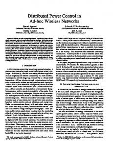
6.4 Dynamic and hybrid algorithms We consider here a hybrid of self-pruning and neighbor-designating algorithms. The first-receipt approach is still used. Upon receiving a broadcast packet from u with designated forward node set D(u) selected by u, v uses the following steps: If v is not a designated forward node and v has not sent the packet before, then v applies the coverage condition to determine its status. If v is a forward node (self selected or designated), v selects a neighbor w 6∈ u ∪ D(u) as its designated forward node (if any) based on a certain priority scheme. A neighbor that covers some nodes in N2 (v) is selected with either the lowest id or the maximum effective node degree (with respect to uncovered nodes in N2 (v)). Node id is used to break a tie in node degree. Then v forwards the packet together with D(v) = {w}. Note that the selected forward neighbor should cover at least one 2-hop neighbor. In this hybrid approach, each node v only uses 2-hop information. Consider the example in Figure 8 and suppose nodes 2 and 9 are forwarding the packet to its neighbors. Using self-pruning, nodes 4 and 6 will be forward nodes and nodes 1 and 3 will be non-forward nodes based on the coverage condition with 2-hop information. It is assumed nodes 1 and 6 receive their first copy of the packet from node 2 and node 4 from node 9. Node 3 receives 23

100

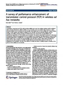
100 links non-forward nodes forward nodes (static) forward nodes (FR) forward nodes (FRB) 80 source node

80

60

60

40

40

20

20

0

links non-forward nodes forward nodes (static) forward nodes (FR) forward nodes (FRB) source node

0 0

20

40

60

80

100

0

20

40

60

80

(a) with 2-hop neighborhood informa-

(b) with 3-hop neighborhood informa-

tion.

tion.

100

Figure 9: Broadcasting on a sample ad hoc network of 100 nodes. The numbers of forward nodes are (a) 49, 45, 41 and (b) 46, 42, 36 for the static, first-receipt, and first-receipt-with-backoff algorithms, respectively. its first copy of the packet from either node 2 or node 9. Using the proposed hybrid approach with node degree as the priority, node 2 is selected as a designated forward node by node 9 and node 6 by node 2. Note that nodes 2 and 9 do not know each other’s forward status and, hence, there is no coordination in selecting their designated forward nodes. Node 4 is no longer a forward node, since nodes 2 and 9 are visited nodes under the local view of node 4 (passed from node 9). If node id is used as the priority in the hybrid approach, node 2 is selected by node 9. Node 3 is selected by node 2, since node 1 does not cover any 2-hop neighbor of node 2. Once node 3 receives the packet, it will pick node 4 to cover node 7. Using the neighbor-designating approach, node 9 selects node 2 first followed by node 4 to complete the 2-hop coverage. Similarly, node 2 selects node 6 and then node 9.

24

7

Simulation

Our simulation study of the generic distributed broadcast protocol focuses on two issues: implementation options that build the local views and special cases of the generic framework. For the first issue, our goal is to find different techniques for local view formation that are appropriate under different network situations, rather than a single optimal combination that applies to all situations. For example, using 3-hop information is more efficient (i.e., has fewer forward nodes) than 2-hop information in static networks or networks with slight mobility, but the overhead of frequent “Hello” messages may be overwhelming in a highly mobile network. An interesting finding is that a proposed dynamic hybrid algorithm outperforms both self-pruning and neighbordesignating algorithms. Seven existing special cases are divided into three groups: static, firstreceipt, and first-receipt-with-backoff, and compared within each group. Usually, self-pruning algorithms outperform neighbor-designating algorithms in the same group, which indicates potential for optimization in neighbor-designating algorithms. In each group, a new algorithm is derived from the generic framework. As the new algorithms combine the strength of existing algorithms, they have the best performance in each group. As our simulation study focuses on broadcast efficiency (i.e., the number of forward nodes), all simulations are conducted on static networks with a collision-free MAC layer. Simulations with a “real” MAC layer, such as IEEE 802.11, are more practical, but we believe the results will not be significantly different. On the other hand, a realistic mobility model and MAC layer is essential in simulations on the broadcast reliability (i.e., the percentage of nodes receiving the broadcast packet). In our custom simulator, each ad hoc network is generated by randomly placing n nodes in a restricted 100 × 100 area. The transmitter range is adjusted according to a given average node degree d to produce exactly

nd 2

links in the corresponding unit disk graph. Two

average node degrees are used in the simulation, one for relatively sparse networks (d = 6) and another for relatively dense networks (d = 18). Networks that are not connected are discarded. For each configuration, the simulation is repeated until the 90% confidence interval of the average value is within ±1%. Figure 9 shows several forward node sets derived from several broadcast algorithms on a sample ad hoc network.

25

d=6, 2-hop 60

Static FR FRB FRBD

50 Number of forward nodes


d=18, 2-hop 60

Static FR FRB FRBD

40 30 20 10

40 30 20 10

0

0 20

30

40

50 60 70 Number of nodes

80

90

100

20

30

40


80

90

100

Figure 10: Performances of broadcast algorithms with different timing options. The average node degree is 6 (left) and 18 (right).

7.1 Implementation options Many existing broadcast algorithms use 2-hop information and node id as priority, because they have the lowest cost in view update. Unless otherwise specified, they are used in the following simulations. Timing. Figure 10 compares performances of different broadcast algorithms, in terms of the size of the forward node set, where each node makes the forward/non-forward decision proactively (Static), after the first receipt of the broadcast packet (FR), after the first receipt with a random backoff delay (FRB), or after the first receipt with a backoff delay that is proportional to the inverse of node degree (FRBD). The static algorithm requires less computation and no extra end-to-end delay, but also produces more forward nodes. The FR algorithm causes no extra end-to-end delay, but recomputes the forward/non-forward status for each broadcasting. FR produces fewer forward nodes than the static algorithm. The two algorithms with backoff delays recompute node status for each broadcasting and cause extra end-to-end delay. They produce the smallest forward node set, and between them, FRBD is slightly better than FRB. Since the computation time is negligible in a broadcast process, the dynamic algorithm is more desirable than the static one. Among the dynamic algorithms, FR is appropriate for highly delaysensitive applications, and FRBD is appropriate for less delay-sensitive applications. Selection. Figure 11 compares performances of different algorithms, where the coverage condition is applied via self-pruning (SP), neighbor-designating (ND), and two hybrid schemes: one that 26

d=6, 2-hop 60

SP ND MaxDeg MinPri



d=18, 2-hop 60

SP ND MaxDeg MinPri

40 30 20 10

40 30 20 10

0

0 20

30

40


80

90

100

20

30

40


80

90

100

Figure 11: Performances of dynamic (first-receipt) algorithms with different selection options. The average node degree is 6 (left) and 18 (right). designates a neighbor with the highest degree (MaxDeg) and the other that designates a neighbor with the lowest id (MinPri). In the neighbor-designating and hybrid schemes, we use the strict rule that every designated node becomes forward node. In relatively sparse networks, the sequence from the worst performance to the best performance is MinPri, ND, SP and MaxDeg. MinPri is the worst, which suggests that designating a neighbor with the lowest priority produces more redundancy than the expected elimination effect. Performances of ND, SP and MaxDeg stay close. MaxDeg is slightly better, because it designates some nodes with large degrees and small id’s, which can be used in replacement paths of nodes that have larger id’s and are originally hard to replace. In relatively dense networks, when the number of nodes is small (n ≤ 50), ND, MinPri and MaxPri stay close and perform better than SP. This is because when the network diameter is small, most broadcast processes complete in 2 hops. In this case, a “centralized” selecting algorithm as used in ND is more effective than the “decentralized” algorithm used in SP. However, in relatively larger networks (n = 100), ND is worse than MinPri and even worse than MaxDeg and SP, because different forward nodes may designate different 1-hop neighbors to cover their common 2-hop neighbors, which causes redundancy in the forward node set. The ND algorithm has the lowest computation cost, because only designated nodes need to compute the forward node set. But ND performs poorly in relatively dense networks. SP, MaxDeg and MinPri have almost the same computation cost, because all nodes are required to check the coverage condition. Among them, MinPri is the worst in all circumstances, MaxDeg is the best in relatively sparse networks, and SP is the best in relatively dense networks. Because the computa-

27

d=6 60

2-hop 3-hop 4-hop 5-hop global



d=18 60

2-hop 3-hop 4-hop 5-hop global

40 30 20 10

40 30 20 10

0

0 20

30

40


80

90

100

20

30

40


80

90

100

Figure 12: Performances of dynamic self-pruning algorithms based on different local views. The average node degree is 6 (left) and 18 (right). tion cost is not as important as the communication cost, MaxDeg and SP are preferable over other algorithms. Note that MaxDeg is a new algorithm derived from the generic framework. Space. Figure 12 compares performances of different algorithms that are based on 2-hop, 3hop, 4-hop, and 5-hop information. Also, performance under global information (Global) is also included as a lower bound. Although the performance progressively improves as the hop count increases, the difference becomes marginal as the hop count increases. In fact, algorithms based on 2- and 3-hop information do not perform significantly worse than the one based on the global information. Considering the cost in gathering neighborhood information, algorithms based on 4-, 5-hop, or global information are not cost-effective compared with the ones based on 2- or 3-hop information. Priority. Figure 13 compares performances of different algorithms using node id (ID), node degree (Degree), and neighborhood connectivity ratio (NCR) as priority values. ID requires no extra maintenance cost but produces more forward nodes. Degree has higher maintenance cost and produces less forward nodes than ID. NCR has the highest maintenance cost and produces the smallest forward node set. Note that in relatively sparse networks, Degree is much better than ID and is very close to NCR. This is because node degree and neighborhood connectivity ratio are better indicators in selecting those nodes in some “critical” positions that are essential in replacement paths of other nodes. When node id is used as the priority, many “non-critical” nodes become forward nodes only because they have higher id’s. In relatively dense networks, all three metrics stay very close. Since there are few critical positions in a dense network, the importance of a good indicator 28

d=6, 2-hop 60

ID Degree NCR



d=18, 2-hop 60

ID Degree NCR

40 30 20 10

40 30 20 10

0

0 20

30

40


80

90

100

20

30

40


80

90

100

Figure 13: Performances of dynamic self-pruning algorithms using different priority values. The average node degree is 6 (left) and 18 (right). is reduced. Considering the cost of collecting and maintaining degree and NCR information, Degree in relatively dense networks and NCR in general has the worst cost-effectiveness. Tradeoffs must be made between performance and maintenance cost in selecting ID and Degree in relatively sparse networks. Overall, there is no single combination of implementation options that is the best for all circumstances. Fine tuning is needed to achieve better tradeoff between performance and overhead based on the types of ad hoc networks and applications.

7.2 Special cases Here we compare performances of several existing special cases of the generic framework, including Dai and Wu’s algorithm (Rule-k), the enhanced Span (Span), MPR, LENWB, dominant pruning (DP), partial dominant pruning (PDP), and SBA. These algorithms can be divided into static and dynamic algorithms, and dynamic algorithms can be further divided into first-receipt and first-receipt-with-backoff algorithms. Each category, except the last one, contains both selfpruning and neighbor-designating algorithms, as shown in Table 1. For the sake of fairness, only algorithms under the same category are compared. Three new algorithms derived from the generic framework using the coverage condition, one for each category, are simulated and compared with existing algorithms. The corresponding performance data of these new algorithms are labelled “Generic” in the result diagrams. 29

Table 1: Existing distributed broadcast algorithms compared in the simulation. Category

Self-pruning

Neighbor-designating

Static First-receipt First-receipt-with-backoff

Rule k, Span LENWB SBA

MPR DP, PDP -

d=6, 2-hop 60

MPR Span Rule k Generic




d=18, 2-hop 60

40 30 20 10

40 30 20 10

0

0 20

30

40


80

90

100

20

30

40

d=6, 3-hop 60

90

100



Number of forward nodes

80

d=18, 3-hop 60


50


40 30 20 10

40 30 20 10

0

0 20

30

40


80

90

100

20

30

40


80

90

100

Figure 14: Performances of several static broadcast algorithms based on 2-hop (the upper row) and 3-hop (the lower row) neighborhood information. The average node degree is 6 (the left column) and 18 (the right column).

30

d=6, 2-hop 60

DP PDP LENWB Generic



d=18, 2-hop 60


40 30 20 10

40 30 20 10

0

0 20

30

40


80

90

100

20

30

40

d=6, 3-hop 60

90

100

90

100




80

d=18, 3-hop 60


50


40 30 20 10

40 30 20 10

0

0 20

30

40


80

90

100

20

30

40


80

Figure 15: Performances of several first-receipt broadcast algorithms based on 2-hop (the upper row) and 3-hop (the lower row) neighborhood information. The average node degree is 6 (the left column) and 18 (the right column). Static algorithms. Figure 14 compares four static broadcast algorithms. All algorithms except MPR use NCR as the priority value, as it is the original configuration of Span. In MPR, the first designator’s transmission time is used to as the priority function in reducing the number of forward nodes. The sequence from the worst performance to the best performance is MPR, Span, Rule k, and Generic. MPR is less efficient in relative dense networks, because of un-coordinated forward node sets designated by different nodes. Span is slightly worse than Rule k, because of its restriction on the length of each replacement path. Generic performs slightly better than Rule k, because it uses the original coverage condition and has no constraint on the lengths of replacement paths; while Rule k only uses the strong coverage condition. First-receipt algorithms. Figure 15 compares three first-receipt broadcast algorithms. All algorithms use node degree as priority values, as it is the original configuration of LENWB. The sequence from the worst performance to the best performance is DP, PDP, LENWB, and Generic. 31

Both DP and PDP are much worse than the other two algorithms, because neighbor-designating in general is worse than self-pruning, and cannot take advantage of the 1-hop priority. PDP is better than DP, since it has fewer 2-hop neighbors to cover than DP does. LENWB is slightly worse than Generic, and can be viewed as a good approximation of Generic. Note that LENWB uses less broadcast state information than Generic. In LENWB, only the last visited node is used in checking the strong coverage condition. In Generic, each node also knows the second last visited node that is piggybacked in the broadcast packet. However, this extra broadcast state information has little impact on performance. A similar observation has also been reported in [28]. First-receipt-with-backoff algorithms. Figure 16 compares two first-receipt-with-backoff algorithms. Generic significantly outperforms SBA, because SBA requires direct neighbor set coverage, while Generic allows indirect coverage. More specifically, a node does not need to forward a broadcast packet even if some of its neighbors are not directly covered by any visited node, but are indirectly connected to a visited node via several intermediate nodes with higher priorities. Overall, within each category, the generic algorithm performs better than existing self-pruning algorithms, which in turn, perform better than existing neighbor designating algorithms.

8

Conclusion

A generic framework of distributed broadcasting in ad hoc networks has been proposed and its correctness has been shown. Four important implementation issues, namely timing, selection, space, and priority, have been discussed and their impacts on broadcast efficiency have been examined. Nine existing broadcast algorithms, which represent a broad spectrum of state-of-art distributed broadcast techniques in ad hoc networks, have been shown to be special cases of the generic framework. Simulation results show that, by adjusting the four implementation options, the generic distributed broadcast protocol can be well adapted to different configurations of ad hoc networks and upper layer applications. We have also shown that several new algorithms can be derived from the generic framework, and that these algorithms produce smaller forward node sets than existing broadcast algorithms under the same requirement of neighborhood information.

32

d=6, 2-hop 60

d=18, 2-hop 60

SBA Generic

SBA Generic



50 40 30 20 10

40 30 20 10

0

0 20

30

40


80

90

100

20

30

40

d=6, 3-hop 60

80

90

100

90

100

d=18, 3-hop 60

SBA Generic

SBA Generic




40 30 20 10

40 30 20 10

0

0 20

30

40


80

90

100

20

30

40


80

Figure 16: Performances of two first-receipt-with-backoff broadcast algorithms based on 2-hop (the upper row) and 3-hop (the lower row) neighborhood information. The average node degree is 6 (the left column) and 18 (the right column).

33

References [1] C. Adjih, P. Jacquet, and L. Viennot. Computing connected dominated sets with multipoint relays. Technical Report 4597, INRIA-Rapport de recherche, Oct. 2002. [2] S. Alagar and S. Venkatesan. Reliable broadcast in mobile wireless networks. In Proceedings of Milcom, pages 236–240, 1995. [3] K. M. Alzoubi, P.-J. Wan, and O. Frieder. Distributed heuristics for connected dominating sets in wireless ad hoc networks. Journal of Communications and Networks, 4(1):22–29, Mar. 2002. [4] B. Chen, K. Jamieson, H. Balakrishnan, and R. Morris. Span: an energy-efficient coordination algorithm for topology maintenance in ad hoc wireless networks. ACM Wireless Networks Journal, 8(5):481–494, Sep. 2002. [5] Y. P. Chen and L. Liestmen. Approximating minimum size weakly-connected dominating sets for clustering mobile ad hoc networks. In Proceedings of ACM MobiHoc, pages 165–172, June 2002. [6] F. Dai and J. Wu. Distributed dominant pruning in ad hoc wireless networks. In Proceedings of IEEE International Conference on Communications (ICC), May 2003. [7] F. Dai and J. Wu. Performance comparison of broadcast protocols for ad hoc networks based on self-pruning. In Procedings of IEEE WCNC, Mar. 2004. Accepted. [8] S. Guha and S. Khuller. Approximation algorithms for connected dominating sets. Algorithmica, 20(4):374–387, Apr. 1998. [9] Z. J. Haas, J. Y. Halpern, and L. Li. Gossip-based ad hoc routing. In Proceedings IEEE INFOCOM, volume 3, pages 1707–1716, June 2002. [10] H. B. Hunt, M. V. Marathe, V. Radhakrishnan, S. S. Ravi, D. J. Rosenkrantz, and R. E. Stearns. NC-approximation schemes for NP- and PSPACE-hard problems for geometric graphs. J. Algorithms, 26(2):238–274, 1998. [11] W. H. Liao, Y. C. Tseng, and J. P. Sheu. GRID: A fully location-aware routing protocol for mobile ad hoc networks. Telecommunication Systems, 18:37–60, 2001. 34

[12] H. Lim and C. Kim. Flooding in wireless ad hoc networks. Computer Communications Journal, 24(3-4):353–363, 2001. [13] C. R. Lin and M. Gerla. Adaptive clustering for mobile wireless networks. IEEE Journal on Selected Areas in Communications, 15(7):1265–1275, 1996. [14] W. Lou and J. Wu. On reducing broadcast redundancy in ad hoc wireless networks. IEEE Transactions on Mobile Computing, 1(2):111–123, Apr.-June 2002. [15] E. Pagani and G. P. Rossi. Providing reliable and fault-tolerant broadcast delivery in mobile ad hoc networks. Mobile Networks and Applications, 4:175–192, 1999. [16] A. Pelc. Handbook of Wireless Networks and Mobile Computing, chapter Broadcasting in radio networks. Edited by I. Stojmenovic, John Wiley & Sons, Inc., Feb. 2002. [17] W. Peng and X. Lu. On the reduction of broadcast redundancy in mobile ad hoc networks. In Proceedings of ACM MobiHoc, pages 129–130, Aug. 2000. [18] W. Peng and X. Lu. AHBP: An efficient broadcast protocol for mobile ad hoc netowrks. Journal of Science and Technology, Beijing, China, 2002. [19] A. Qayyum, L. Viennot, and A. Laouiti. Multipoint relaying for flooding broadcast message in mobile wireless networks. In Proceedings of the 35th Annual Hawaii International Conference on System Sciences (HICSS), volume 9, page 298, Jan. 2002. [20] V. Ramasubramanian, R. Chandra, and D. Mosse. Providing a bidirectional abstraction for unidirectional ad hoc networks. In Proceedings of IEEE INFOCOM, volume 3, pages 1258– 1267, June 2002. [21] M.A. Spohn and J.J. Garcia-Luna-Aceves. Enhanced dominant pruning applied to the route discovery process of on-demand routing protocols. In Proc. IEEE IC3N 03: Twelfth International Conference on Computer Communications and Networks, Oct. 2003. [22] I. Stojmenovic. Handbook of Wireless Networks and Mobile Computing, chapter Location Updates for Efficient Routing in Ad Hoc Networks. Edited by I. Stojmenovic, John Wiley & Sons, Inc., Feb. 2002.

35

[23] I. Stojmenovic, M. Seddigh, and J. Zunic. Dominating sets and neighbor elimination based broadcasting algorithms in wireless networks. IEEE Trans. on Parallel and Distributed Systems, 13(1):14–25, Jan. 2002. [24] J. Sucec and I. Marsic. An efficient distributed network-wide broadcast algorithm for mobile ad hoc networks. CAIP Technical Report 248, Rutgers University, Sep. 2000. [25] Y.-C. Tseng, S.-Y. Ni, Y.-S. Chen, and J.-P. Sheu. The broadcast storm problem in a mobile ad hoc network. Wireless Networks, 8(2/3):153–167, Mar.-May 2002. [26] P. J. Wan, K. Alzoubi, and O. Frieder. Distributed construction of connected dominating set in wireless ad hoc networks. Proceedings of IEEE INFOCOM, 3:1597–1604, June 2002. [27] J. Wu. Extended dominating-set-based routing in ad hoc wireless networks with unidirectional links. IEEE Transactions on Parallel and Distributed Systems, 13(9):866–881, Sept. 2002. [28] J. Wu and F. Dai. Broadcasting in ad hoc networks based on self-pruning. International Journal of Foundations of Computer Science, 14(2):201–221, Apr. 2003. [29] J. Wu and F. Dai. A generic distributed broadcast scheme in ad hoc wireless networks. In Proceedings of ICDCS, pages 460–468, May 2003. [30] J. Wu and F. Dai. Mobility management and its applications in efficient broadcasting in mobile ad hoc networks. In Procedings of IEEE INFOCOM, Mar. 2004. Accepted. [31] J. Wu and H. Li. On calculating connected dominating set for efficient routing in ad hoc wireless networks. In Proceedings of the 3rd International Workshop on Discrete Algorithms and Methods for Mobile Computing and Communications (Dial M), pages 7–14, 1999. [32] J. Wu and W. Lou. Forward-node-set-based broadcast in clustered mobile ad hoc networks. Wireless Communication and Mobile Computing, special issue on Algorithmic, Geometric, Graph, Combinatorial, and Vector, 3(2):155–173, 2003.

36