Distributed Topology Control in Wireless Ad Hoc Networks using β ...

1

Distributed Topology Control in Wireless Ad Hoc Networks using β -Skeletons Manvendu Bhardwaj, Satyajayant Misra and Guoliang Xue

Abstract— We propose a novel approach for sparse topology generation in wireless ad hoc networks based on a graph structure known as β-skeletons. Two efficient algorithms are presented in this paper for creating a connected topology from an underlying β-skeleton. One algorithm is a distributed algorithm that runs on each component of the β-skeleton. It creates a connected structure from the disconnected β-skeleton graph using a distributed leader election algorithm. The running time of this algorithm is O(n log n). The other is a localized algorithm that uses two-hop neighborhood information to generate a connected topology, with a running time of O(n). Simulations show consistent decrease in node degree in the resulting topology. The observed decrease is greater than 33% in comparison to the Relative Neighborhod Graph (RNG) and greater than 50% in comparison to other topology structures such as, the Gabriel Graph (GG) and the Yao construction on GG. Index Terms— Wireless ad hoc networks, topology control, bounded degree, localized algorithm, distributed algorithm.

I. I NTRODUCTION Recent technological advances in wireless ad hoc and sensor networks have made large scale deployment possible. As a result there is a need to reduce contention for the medium by a large number of sensors for higher network throughput. Topology control is used for this purpose. Using topology control, each node in the network can choose a set of neighbors to which it shall be connected and adjust its transmit power level. The reduced power levels of transmission can also help in reducing interference. Topology control aims at making the underlying topology sparse, while maintaining the desirable properties [2]. Many constructions for topology control like the Relative Neighborhood Graph (RNG), the Gabriel Graph (GG), and the Yao Graph have been proposed in existing literature [16]. In this paper we study topology control in wireless ad hoc networks using a more general family of graphs known as β-skeletons [16]. Both RNG and GG are members of this family. The general class of β-skeletons have not been used for topology control as these graphs are not guaranteed to be connected. We propose two distributed algorithms to generate a connected topology. The first algorithm uses a distributed leader election algorithm and distributed Depth First Search This research was supported in part by NSF grants CCF-0431167, ARO grant W911NF-04-1-0385, and a seed grant from CEINT. The information reported here does not reflect the position or the policy of the federal government. All three authors are with the Department of Computer Science and Engineering, Arizona State University, Tempe, AZ 85287-8809. Email: {manvendu, satyajayant, xue}@asu.edu.

(DFS) to create a connected graph. While, the second algorithm is a localized algorithm that uses two-hop neighborhood information for connecting the β-skeleton components. The remainder of the paper is organized as follows. In the Section II, we describe related work in the area of topology control. In Section III, we present the concepts used in the paper. In Section IV, we present two distributed algorithms for constructing connected topology based on β-skeletons. In Section V, we analyze the proposed algorithms. Section VI presents simulation results and observations. We conclude this paper in Section VII. II. R ELATED W ORK One of the first distributed topology control algorithms that reduce interference wasproposed in [12]. In [9] the authors propose topology control in multi-hop wireless networks using transmit power adjustment. Wieselthier et al. in [10] introduce energy efficient algorithms for tree construction in a wireless network using wireless multicast advantage. In [8] the authors give a detailed analysis of a distributed cone based algorithm for topology control. In [2], Wang and Li propose an algorithm that constructs a bounded degree planar spanner for wireless ad hoc networks. Song et al. extend the idea proposed in [1] by introducing two new localized algorithms for constructing energy efficient routing structures. The first structure is a bounded degree planar power spanner, obtained by a Yao construction on a GG. The second structure is a degree-k (k > 8) planar power spanner. A Local Minimum Spanning Tree (LMST) based approach is proposed in [4]. XiangYang Li et al. in [19] use a localized method to construct a bounded degree planar graph whose total edge length is within a constant factor of the minimum spanning tree (MST), bounding the degree of any node to atmost 6. III. BACKGROUND AND C ONCEPTS This section gives a brief overview of β-skeletons, an outline of other geometric structures for topology control and presents the network model used. A. β-skeletons β-skeletons [16] are a family of graphs whose structure is based on the measure of the empty neighborhoods around the edges of the graphs. A β-skeleton of a set of points is a graph defined to contain exactly those edges (v, w) such that: • if β > 1, then the union ∪ of two circles, each having v, w as a chord and having diameter distance(v, w) × β contains no points other than v and w.

2

•

•

if β = 1, then the circle having (v, w) as diameter contains no points other than v and w. if 0 < β < 1, then the intersection I of two circles each with v, w as a chord and having diameter distance(v, w)/β contains no points other than v and w.

knows its position. In our algorithms every node should know the relative position of its one-hop neighbors (by one-hop broadcast). Further, in our model we assume that there is no packet loss in the network. In this paper we focus only on the generation of initial topology. Maintenance of topology as a result of node failure, movement, etc. is a topic for future study. IV. P ROPOSED A PPROACHES

v

w v

w

v

w

A

(a)

(b)

(c)

v

(d) Fig. 1. (a) β-skeleton; (b) RNG Graph; (c) Gabriel Graph; (d) YaoGG graph

The value of β can be used to control the sparseness of the graph, higher the β value, more sparse the graph. For β > 1, however, the β-skeleton is not guaranteed to be connected. The relative neighborhood graph (RNG) of a set V of points in Euclidean space is the graph (V, E), where (p, q) ∈ E iff there is no point z ∈ V such that d(p, z) < d(p, q) and d(q, z) < d(p, q). The Gabriel Graph (GG) is defined as the graph G(V, E), where (p, q) ∈ E iff there is no other node z within the circle drawn with (p, q) as the diameter. The Yao on Gabriel graph (YaoGG) is an extension to the Gabriel Graph. Figure 1. depicts each of these graphs. B. Desirable properties of topology control structures The following are some of the desired properties for a topology in a wireless ad hoc network: • Sparseness • Bounded node degree • Planarity 1 • Spanner Property • Localized construction C. Network Model A wireless ad-hoc/sensor network consists of a set V of n wireless nodes randomly distributed in a two-dimensional plane. Each node has the same maximum transmission range R. Given proper scaling we can assume that all nodes have the maximum transmission range equal to one unit. Thus, these wireless nodes define a Unit Disk Graph, UDG(V). We also assume all nodes have distinctive identities and each node 1 A subgraph H of graph G is called a power spanner of a graph G if there is a positive real constant ρ (power stretch factor) such that for any two nodes, the power consumption of the shortest path in H is at most ρ times of the power consumption of the shortest path in G.

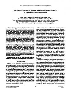
We propose a novel method to build power efficient planar structures with comparable communication costs and lower node degree bounds as compared with previously best known planar power efficient structures [1]. As a first step our algorithm constructs a β- skeleton and RNG in a localized fashion. The idea behind this construction is similar to localized construction of Gabriel Graph presented in [1]. We define the concept of Lune(u, w) for the vertices u and w of a graph as the intersection of two circles with radius dist (u, w) centered at points, u and w respectively. Further, we use the term N (u, v, β) defined as the neighborhood of the vertices u and v in the β-skeleton. A. Algorithm 1: Constructing UDG, RNG and β-skeleton Components Let EU DG (u), ERN G (u) and EBS (u) be the set of edges adjacent to node u in the UDG, RNG and the β-skeleton respectively. To start, each node u sets EU DG (u), ERN G (u) and EBS (u) to be empty. 1) Each node u locally broadcasts a message with its ID and its position (x,y) to all nodes in its transmission range. 2) If u gets a message from another node v, then it does the following: • Adds the edge (u, v) to EU DG (u). • Checks if there is another edge (u, w) in EU DG , where w is inside lune(u,v). If no such edge (u, w) exists then u adds edge (u, v) to ERN G (u). • Checks if there is another edge (u, w) in EU DG , where w is inside (N(u, v, β). If no such edge (u, w) exists then u adds edge (u, v) to EBS (u). • Node u checks if v is in (N(u, w, β) of some other edge (u, w) in EBS (u). If YES, it removes (u, w) from EBS (u). • Node u checks if v is in (lune(u, w) of some other edge (u, w) in ERN G (u). If YES, it removes (u, w) from ERN G (u). Node u repeats 2 until no new messages are received. The structure we get as a result of the above algorithm is not connected. The following sub-sections describes two algorithms to generate a connected topology in a distributed and localized fashion, from the components generated by the above construction. Figure 2 shows the construction of the YaoGG and the corresponding β-skeleton for a randomly chosen network topology. The black lines represent the edges in the β-skeleton and the red edges show the significant number of extra edges that exist in the YaoGG in addition to the black edges.

3

iii) Finally each node v on receiving a delete-edge message from u deletes u from Neighbors(v) in the final topology. iv) Node v repeats this until no other CCI packet is received. 4) Each node reduces its transmission power level, and sets it based on its longest outgoing edge. C

A

Fig. 2.

YaoGG and Connected β-skeleton comparison

C’

B D’

B. Algorithm 2: Two-hop Neighborhood Leader based Algorithm (2NBA) This localized algorithm decides which, edges from RNG to use for connecting the disconnected β-skeletons, based on two-hop neighborhood information at each node. We define, NBS (u) as the set of immediate neighbors of u (including itself) in the β-skeleton obtained from Algorithm 1. Also, we define, NRN G (u) as the set of immediate neighbors of u in the RNG obtained from Algorithm 1. A total neighborhood of u is also defined, Neighbors(u), this set is initialized to all nodes in NBS (u). 1) Two-hop Leader Election: Each node u stores the largest ID among all nodes in NBS (u) as its potential leader, PL(u). u broadcasts its PL(u) to all its immediate neighbors. A node v on receiving the PL(u) information from all its neighbors (u), sets its final LocalLeaderID (v) as max(PL(u)) for all u in NBS (v). 2) RNG edge selection: Each node u broadcasts its NodeID and LocalLeaderID to all nodes v in NRN G (u). a) Each node v on receiving the NodeID and LocalLeaderID from its RNG neighbor u, adds u to Neighbors(v) if LocalLeaderID (u) 6= LocalLeaderID (v). 3) Edge Pruning: a) Each node u generates a connected component information (CCI) packet containing its ID and the LocalLeaderID (v) of all nodes it connects to in Step 2. The packet has a Time To Live (TTL) field with its value set to 4. b) Each node v on receiving a CCI packet from u does the following : i) if LocalLeaderID (w) of any of its neighbors w in Neighbors(v) is equal to any LocalLeaderID in the CCI packet and NodeID(u) > NodeID(v) it broadcasts a delete-edge message to all such w. ii) if TTL > 0 v decreases the TTL value in the packet by 1 and broadcasts the packet to all u in Neighbors(v). else it drops the CCI packet.

Fig. 3.

Node degree in a β-skeleton

C. Algorithm 3: Complete Neighborhood Leader based Algorithm (CNBA) The basic idea behind this algorithm is that each disconnected β-component elects a leader on the basis of node ID. 1) Leader Election: A leader is elected in each of the βskeleton components using a distributed leader election protocols like [17]. After the election each component is assigned a Component ID, which is the ID of the leader (largest ID node in the component). The leader election protocol uses only edges that are a part of the constructed β-skeletons. Due to space limitation details are omitted here. 2) Step 1 - Depth First propagation of component ID: The elected leader is responsible for propagating its own ID as the β component ID to all the nodes in the βcomponent. Thus each connected β-component is now identified by its component ID. 3) Step2 - Components Connection: At the end of Step 1 each node in a component knows its component ID. The following algorithm is executed at each component to ensure connectivity of the overall graph. a) Each node, u broadcasts its component ID to all nodes in NRN G (u). b) If for a receiving node ComponentID(v) 6= ComponentID(u), a v adds u as its neighbor the v also store componentID(u). 4) Step 3 - Edge pruning: The leader node of a βcomponent sends out a message containing the component IDs of the other β-components it is connected to. The message is propagated using the DFS tree generated in step 1. Each node u on receiving the message does the following: • For all neighbors v of u if component ID(v) is equal to any of the component IDs in the received message, u broadcasts a delete-edge message containing the node IDs of all such v.

4

If for any neighbor v of u componentID(v) is not equal to any componentIDs in the message adds the componentIDs of all such v’s to the message. • Node u sends the updated message to its DFS successor. • Lastly, any node v receiving the delete-edge message from u deletes u from its neighbor list in the final topology. 5) Each node reduces its transmission power level, and sets it based on its longest outgoing edge. •

B. Message Complexity of CNBA The message complexity of Leader election algorithm is n lg n+|E|, where n is the number of vertices and |E| number of edges. Step 1 has a complexity of O(n) as it is DFS traversal of the tree formed from the Leader Election Algorithm. Step 2 has a complexity of O(n) and step 3 has a complexity of O(n) again. So the total message complexity is bounded by n lg n + |E|. The number of edges, |E| in a β-skeleton is bounded from above by the number of edges in a RNG for the same graph which, is 3n-6. Hence the message complexity of CNBA is O(n lg n).

V. A NALYSIS Theorem 1: The minimum angle between two edges (u, v) and (u, w) of a β-skeleton for a node u and the neighboring nodes v and√w is given by (π − α)/2, where sin(α) = 1/β, and β > 2/ 3. Proof: As shown in figure 3. Let AB be an edge in the βskeleton. So for an edge AB to exist, no node can lie in the circle based neighborhood N(A, B, β). Let C is a point such that, 6 BAC = (π − α)/2. Lets assume that there exists a node C’ such that 6 BAC ′ < 6 BAC. By the definition of β-skeletons, only the following 2 cases are possible: • Case 1: C’ lies on the periphery of the circle based neighborhood √ N(A, B, β): For β ≥ 2/ 3, 6 ACB = α (≤ π/3). Therefore, AC’ > AB. Therefore, if a circle based neighborhood N(A, C’, β) is drawn for AC’ (as AB in figure 4). B will always lie in the interior of the neighborhood.Hence, edge AC’ can not exist. • Case 2: C’ lies beyond the periphery of N(A, B, β): Here the length of AC’ is even more than that considered in case 1. Therefore, again B would lie in the interior of N(A, C’, β). So, edge AC’ can not exist. Hence we conclude, that the minimum value of 6 BAC ′ = 6 BAC. Where 6 BAC = (π − α)/2. This concludes the proof. Corollary 1: Maximum √ node degree of a β-skeleton is 4π ⌊ π−α ⌋, where β ≥ 2/ 3. Proof: Directly follows from theorem 1. A. Message Complexity of 2NBA The message complexities of the steps are as follows: • β-skeleton, UDG and RNG construction: As each node broadcasts its location information only once, this step requires n messages. • Two hop leader election: Each node broadcasts its PL(u) information. This step also requires n messages. • RNG edge selection: Each node broadcasts one message to all its RNG neighbors requiring a total of n messages. • Edge Pruning: Each node generates a CCI packet for its β-skeleton neighbors with a TTL value of 4 hops. 4π ⌋ From corollary 1, each node has a maximum of ⌊ π−α neighbors. Therefore, this step requires a maximum of 4π ⌋)3 n. (⌊ π−α 3

4π Hence message complexity of 2NBA is (⌊ π−α ⌋ + 3)n, i.e., O(n).

VI. S IMULATION AND R ESULTS We evaluate the topology generated by our algorithm for: Power Spanning Ratio, Average and Maximum node degree and Number of edges. The results are compared with that from RNG, GG and YaoGG graphs. A. Simulation Setup The setup consists of n nodes spread randomly in a square region of size 30×30. All nodes are assigned a maximum transmit (Tx) power 10. A UDG is generated by connecting two nodes u and v if they are in each other’s Tx region, given by d(u, v)α , α = 2 is the attenuation factor. From the UDG the GG, RNG, YaoGG and the two β-skeleton graphs, obtained from CNBA and 2NBA are constructed. The properties of the graphs were studied by varying number of nodes from 30 to 300 in increments of 30. For a given number of nodes the simulation was run for 100 iterations to allow convergence. The value of k used for YaoGG was 9 and the value of β used √ was 2. B. Analysis of Results 1) Power Spanning Ratio: Figure 4 shows the comparison of the average power spanning ratio (power stretch factor). The power spanning ratio for CNBA and 2NBA is higher than that of YaoGG / GG as only a small subset of the RNG edges are used to connect the β-skeleton. But, results in an average increase of the number of hops from a source to destination. 2NBA fares better than CNBA because of extra edges that added due to the use of two hop information for connection of the β-skeleton. 2) Node Degree: A smaller, bounded node degree is an extremely desirable property. Both CNBA and 2NBA perform significantly better (almost twice) than any other (figure 5) scheme as we use a sparse β-skeleton graph and connect it. CNBA performs better than 2NBA because, in CNBA each component may connect to another only once. CNBA and 2NBA perform better in average node degree as well (figure 6). 3) Number of Edges in the Graph: Figure 7 shows the number of edges. Both CNBA and 2NBA √ have lesser edges than YaoGG or GG. We have used β = 2 which separates the graph into small components with average maximum number of hops of value 4. Hence, both the CNBA and the 2NBA give almost similar results.

5

3 RNG GG YaoGG CNBA 2NBA

RNG GG YaoGG CNBA 2NBA

1400

1200

Average Power Spanning Ratio

2.5

Number of edges

1000

2

800

600

400

1.5

200

0

1 0

Fig. 4.

50

100

150 Number of nodes

200

250

Fig. 7.

Average Power Spanning Ratio

RNG GG YaoGG CNBA 2NBA

Maximum node degree

14

12

10

8

6

4

Fig. 5.

50

100

150 Number of nodes

200

250

300

Maximum Node Degree

10 RNG GG YaoGG CNBA 2NBA

9

Average node degree

8

7

6

5

4

3 0

Fig. 6.

50

100

150 Number of nodes

200

250

50

100

150 Number of nodes

200

250

300

Number of Edges in Graph

R EFERENCES

16

0

0

300

300

Average Node Degree

VII. C ONCLUSIONS AND F UTURE W ORK In this paper we have explored the use of β-skeletons as a topology control structure in wireless ad hoc networks. We propose two algorithms to make the β-skeletons connected. Our algorithms perform significantly better than other well known existing topology control structures. We intend to extend our work in future to focus on application of this topology control structure under real traffic conditions. We plan to optimize the algorithms for a dynamic topology.

[1] W.Z Song, Y.Wang, X-Y Li and O.Frieder, ”Localized Algorithms for Energy Efficient Topology in Wireless Ad Hoc Networks”, in The fifth ACM International Symposium on Mobile Ad Hoc Networking and Computing (MobiHoc) ’04, 2004. [2] Yu Wang and Xiang-Yang Li, ”Localized Construction of Bounded Degree and Planar Spanner for Wireless Ad Hoc Networks”, in DIALMPOMC ’03, 2003 [3] Baruch Awerbuch, ”Optimal Distributed Algorithms for Minumum Weight Spanning Tree, Counting, Leader Election and related problems”, in Annual ACM Symposium on Theory of Computing, 1987. [4] Baruch Awerbuch, ”Applications of k-Local MST for Topology Control and Broadcasting in Wireless ad Hoc Networks”, in IEEE Transaction on Parallel and Distributed Systems (TPDS), 2004. [5] Martin Burkhart, Pascal von Rickenbach, Roger Wattenhofer and Aaron Zollinger, ”Does Topology Control Reduce Interference?”, in MobiHoc ’04, 2004. [6] Ning Li and Jennifer C. Hou, ”Topology Control in Heterogeneous Wireless Networks: Problems and Solutions”, in IEEE INFOCOM ’04, 2004. [7] Ning Li, Jennifer C. Hou and Lui Sha, ”Design and Analysis of an MSTBased Topology Control Algorithm”, in IEEE INFOCOM ’04, 2004. [8] Li Li, Joseph Y. Halpern, Paramvir Bahl, Yi-Min Wang and Roger Wattenhofer, ”Analysis of a Cone-Based Distributed Topology Control Algorithm for Wireless Multi-hop Networks”, in Microsoft Research MSR-TR-2001-53, 2001. [9] Ram Ramanathan and Regina Rosales-Hain, ”Topology Control of Multihop Wireless Networks using Transmit Power Adjustment ”, in IEEE INFOCOM ’00, 2000. [10] Jeffrey E. Wieselthier, Gam D. Nyugen and Anthony Ephremides, ”On the Construction of Energy-Efficient Broadcast and Multicast Trees in Wireless Networks”, in IEEE INFOCOM ’00, 2000. [11] Intae Kang and Radha Poovendran, ”Maximizing Static Network Lifetime of Wireless Broadcast Adhoc Networks”, in IEEE International Conference on Communications, (ICC) ’03, 2003. [12] Limin Hu, ”Topology Control for Multihop Packet Radio Networks”, in IEEE Transactions on Communications, Vol. 41, No. 10, 1993. [13] Piyush Gupta and P.R. Kumar, ”The Capacity of Wireless Networks”, in IMA Workshop on Applied Probability at the Chinese University of Hong Kong, 1999. [14] R. G. Gallagher, P. A. Humblet and P. M. Spira, ”A Distributed Algorithm for Minimum-Weight Spanning Trees”, in ACM Transactions on Programming Languages and Systems (TOPLAS), 1983. [15] I.F. Akyildiz, W. Su, Y. Sankarasubramaniam, E. Cayirci, ”Wireless Sensor Networks: A Survey”, in Computer Networks, 2002. [16] David G. Kirkpatrick and John D. Radke, ”A Framework for Computational Morphology”, in ACM/Kluwer Wireless Networks, 2001. [17] Navneet Malpani, Jennifer L. Welsh and Nitin Vaidya, ”Leader Election Algorithms for Mobile Ad Hoc Networks”, in DIAL-M Workshop, 2000. [18] Brad Karp and H. T. Kung, ”Gpsr: Greedy perimeter stateless routing for wireless networks”, ACM/IEEE International Conference on Mobile Computing and Networking (MobiCom), 2000. [19] Xiang-Yang Li, Yu Wang, Peng-Jun Wan, Wen-Zhan Song and Ophir Frieder, ”Localized Low-Weight Graph and Its Applications in Wireless Ad Hoc Networks”, IEEE INFOCOM ’04, 2004.