models in ATM switches with queues at the end. A new model based on cell loss is presented in section 3. Next, section 4 introduces a genetic algorithm to solve ...
A GENETIC ALGORITHM BASED ON CELL LOSS FOR DYNAMIC ROUTING IN ATM NETWORKS 1
1
1
P Cortes , J Muñuzuri , J Larrañeta and L Onieva
1
1
Seville University, Escuela Superior Ingenieros. Grupo Ingeniería Organización. Camino de los Descubrimientos s/n. Sevilla 41092. Spain.
Abstract. New B-ISDN will have to ensure a high standard of quality of service measured as delay in the communications, guarantee of safety communications and of course no loss of information. Although the routing optimization problem has been previously dealt with in the bibliography, not many works have been presented according to the routing in ATM networks using cell loss as the overall criterion. Here a new model based on cell loss is presented for an ATM network with matrix switches and queues at the end. A quickly evaluated genetic algorithm is proposed to solve the model.
1 Introduction In the near future telecommunication networks with higher capacity and speed will be needed to give solution to the set of transport and traffic volume requirements. In the eighties of the past century, the ITU-T recommended the adoption of Asynchronous Transfer Mode (ATM) as switching mode and the Synchronous Digital Hierarchy (SDH) as transmission mode for the future broadband network. In this context, the routing algorithms will have to ensure a high standard of quality of service measured as delay in the communications, guarantee of safety communications and of course no loss of information. Several references based on soft computing techniques can be found dealing with the routing operation, most of them are based on circuit or packet switched networks. So, diverse authors (e.g. [5] or [12]) have shown the use of neural approaches to solve the real time traffic routing problem. A fuzzy multiobjective optimization model to develop a routing algorithm to guarantee the various quality of service characteristics requested by the wide range of applications supported by B-ISDN has been presented in [1]. The use of cutting planes has been analyzed to deal with the routing problem with capacity limitations, [4]. A hybrid neuralgenetic procedure to deal with the bandwidth allocation of virtual paths in ATM networks has been developed in [3]. Here we propose the use of a genetic algorithm to route the communications in an ATM operation mode ensuring no relevant loss of information through a new model based on cell loss. The rest of the paper deal with the ATM mode description in section 2, including the different time scales to be considered in ATM operation and the loss models in ATM switches with queues at the end. A new model based on cell loss is presented in section 3. Next, section 4 introduces a genetic algorithm to solve
the problem. Section 5 shows the results in randomly generated and real life problems. Finally, we review the main aspects in the latest section.
2 The Asynchronous Transfer Mode The Asynchronous Transfer Mode (ATM) was created to provide fastest communications in both public and private networks. ATM can be characterized as a hybrid between circuit and packet switched networks, [11]. ATM combines circuit and packet switched networks maintaining the channel structures, by means of timeslot division, as in circuit switched, and the packet structure, by means of ATM cells, as in packet switched. ATM cells are 53 bytes sized, 5 bytes for the header and 48 bytes for the payload. Into the header, the VCI (Virtual Channel Identifier) and VPI (Virtual Path Identifier) fields specify the circuit and path that each cell should flow. The VPI and VCI identifiers are only valid into each connection link, and acts identifying a logic circuit into the physical link, see figure 1. When the cell arrives to the switch, the VPI/VCI are found into the routing tables and the cell is routed trough the output port changing the identifier when necessary. The virtual circuit (or channel) concept is an abstraction representing the cell unidirectional transport associated to an identifier (VCI). The VCI as the VPI indicate an ordered cell flow associated to a concrete connection. The virtual connection channel (VCC) concept means the connection of the different virtual paths from the origin of communication until the destination of communication, as next figure 1 depicts.
Fig. 1. Virtual circuits, virtual paths and virtual connection channel
Into the switches, the communication is transported from an inflow logic channel into an outflow logic channel. This procedure is known as routing. Cell loss in ATM switches appears when very much cells are routed onto the same link, being higher the cell number than the switch buffer size. Habitual -8 -11 values for cell loss probability are from 10 to 10 . The switches can be classified in accordance with the structure of the switching fabric architecture. The matrix switch is one of the most recommended switches, where a connection matrix establishes the interconnection of any input point with any output point. One of the better delay-performance relations is obtained for matrix switches with queues at the end. This option allows transmit more than one cell in the same timeslot. To ensure no cell loss the transference must be N (number of input ports) times faster than the cell homing rate. Moreover, the queue location at the end avoids the line header blocking.
The ATM service categories are four. Constant Bit Rate service (CBR) to maintain real time communications as video or audio with very strict delay requirement. The CBR service provides a connection with large bandwidth and very low cell loss probability. Variable Bit Rate service (VBR) indicated for frame relay traffic. Available Bit Rate service (ABR) used for unknown characteristics traffic and moderately restrictive attending to cell loss and without delay requirement as real time applications. Finally, Unspecified Bit Rate service (UBR) to use the remaining available bandwidth. 2.1 Time scales in ATM networks The traditional Erlang model considers one unique time scale: the connection scale or call scale. In bandwidth traffic this only consideration is not possible. At this respect, a detailed study is done in [10], considering three time scale levels: the call level, the burst level and the cell level proposing a control procedure acting at the burst and call level. Here, we consider the cell level necessary to deal with the switch cell loss analysis, so the flow variables must be referred to the cell level scale. In addition, we consider the call level to ensure the call routing. In ATM, once the first cell is routed onto a virtual circuit all the remaining cells follow the first one through the same circuit, so the path variables must be referred to the call level scale. Figure 2 reveals the different levels and their interrelations. 1LYHO�GH�OODPDGD��FDGD�UDQXUD�UHSUHVHQWD�HO�WLHPSR “Call level: each slot represents the average time for a call” PHGLR�GH�GXUDFLyQ�GH�XQD�OODPDGD��W�
�
�
�
�
�
7
���������� W
“Cell level: each 1LYHO�GH�FpOXOD��FDGD�OODPDGD�VH�GLYLGH�HQ�XQ�FRQMXQWR�GH�FpOXODV� call is divided into a set of cells. Each one of them is assigned to a fixed time” &DGD�XQD�GH�HOODV�RFXSD�XQ�WLHPSR�ILMR�
Fig. 2. Timescales in ATM networks
The cell loss function depends on the switch internal structure. In our case, we are considering matrix switches with queues at the end. In ATM switches, the transmission time for one cell is measured as a slot, approximately 2.8 Pseg at 155.52 Mbps. The ATM networks are synchronized, so when a cell leaves the buffer at the end of the slot, it is synchronized and served at the beginning of the following slot. The cell arrivals can take place in any instant during a slot. The precise arrival instant is no relevant because the cells arriving during the slot n will not leave the buffer before the slot n+1. We use the term port to designate each of the inputs and outputs at the switch, so we deal with input ports and output ports relative to the input links and the output links. We will use independently the terms port or link. The following figure 6 depicts the previous description.
Input port, -3XHUWRV�GH� HQWUDGD� 3 li
OL
Switch (node) i 1RGR�L
Output port, -ij
3XHUWRV�GH VDOLGD�3LM
5HG�GH�LQWHUFRQH[LyQ
Switching fabric
Fig. 3. Ports in an ATM switch
2.2 Cell loss model in ATM networks In ATM networks, each switch is composed by a set of buffers and a switching fabric. The buffers are finite capacity queues where the cells wait to be served; each buffer can be well modeled as a Markov chain. The switching fabric can be implemented by means of an interconnection matrix, central memory, bus or interconnection ring. Therefore, the problem can be assimilated to a queuing system. In this line, the cell loss rate, / , is described in [11] as
/
(� N � U
(1)
Being U the average number of served cells per timeslot and E(K) the expected cell number arriving to the system. According to these expressions we can obtain the total number of lost cells in each switch output port, supposing size-b buffers in a timeslot and measured as cells/slot. We note this cell loss function as LijW(O) meaning the cell loss in the output port j, relative to the switch i in the instant • when the arrival rate is •. It is habitual to use the cell loss probability (CLP) calculated as CLP=L/E(k) or the cell loss rate (CLR) calculated as the total lost cells with respect to the total transmitted cells during a period. In this paper, we make use of the total cell loss as the objective function for evaluating the routing options, as well as the CLR. Finally, we have to remark that the buffer size is a critical parameter. Each ATM switch must have a size of queue enough to ensure low cell loss and low delay conditions. These two conditions are opposing. Next figure 8 represents the CLP versus the queue capacity. It can be appraised how a not very large queue size guarantees acceptable CLP. Anyhow, we implement a buffer size based on standard sizes for control admission call, [6], as can be seen in the appendix.
Fig. 4. Cell loss probability versus queue size
3 Model based on cell loss ATM networks can be well suited by graphs G = (N, E) being N the set of nodes or switches and E the set of links. Many research has been done under the perspective of minimizing the delay [2], in such cases the only delay considered is the delay into the switch due to the queue and the real switching process because the rest of sources of delay, electric-optic conversion or signal propagation, are second order factors. ATM cells can be lost through four manners: due to line transmission failures, Usage Parameter Control (UPC) in the switching network, buffer sizes or switching fabric limitation. We consider as cell loss only those inside the switch. It is not a strong limitation because it represents the largest part of the cell loss in ATM networks. Moreover, in our model, we consider only CBR traffic, also this is not a strong restriction because of VBR, ABR and UBR traffic are much less restrictive with the quality conditions according to cell loss (our objective function). Under these conditions, the input data are the network topology and the demand of communication under CBR service conditions and the maximum allowed cell loss. Moreover, we assume links of extra capacity. It is a realistic supposition because telecommunication links are over dimensioned due to the prevision of future traffic increments. So here, we do not consider the capacity problem. Parameters: N Set of nodes (switches). E Set of links. M Set of communication origin-destination pairs (O(m) origin of communication m and D(m) destination of communication m). H(m) Set of feasible paths to connect each origin-destination pair m. T Temporal horizon at call scale. This horizon is composed by call time division W 7 . Subsequently, the call time scale is divided into the cell time scale, W W . N(h) Set of nodes belonging to path h. E(h) Set of links belonging to path h. B(i) Set of nodes located before node i. A(i) Set of nodes located after node i. Variables: m,t Ph Binary variable indicating if the connection between the origin and destination of communication O(m) and D(m) is established by the path h, referred at the call scale W 7 . m, Xh,ij W Continuous flow variable (cell/slot) associated to the pair m over the link (i,j) in the expressed direction (from i to j), being (i,j) a link of the path h, referred to the cell scale. m, lh,ij W Continuous variable (cell/slot) determining the cell loss at the link (i,j) due to the port j into the switch i in the connection path h used by the pair of communication m, in the timeslot W W (so it is referred to the cell scale). FijW Total cell flow variable (cell/slot) that should be routed from node i to node j. It is referred to the cell scale W W .
It is important to note the difference between the variables FijW and Xh,ij W. The first of them refers to the total flow of cells that ideally should go through the link (i,j), supposing no cell loss, meanwhile the second variable has in account the cell loss possibility. Next figure 5 depicts an example. The switches v, w, y, z are previously located to the node i, and the nodes j, k are located after the node i. For an instant •, there is a flow of cells from nodes v, w, y, z to the node i, the flow from nodes v, z must be routed to the node j meanwhile the flow from nodes w, y must be routed to the switch k. m,
;K��YLP��WW
Y
Z \
;K��ZLP��WW
6
;K��\LP���WW
]
$P��W
6
)LMW
)LN W
3LM
3LN
OK�LM P�W OK�LN
;K�LM P��WW ;K�LNP��WW
P�W
;K��]LP���WW
Fig. 5. Total flow and cell loss into the switch
Demand of the origin-destination pair m in the timeslot W W . It is referred to the cell scale and expressed in cell/slot. GoSm Grade of service. Maximum number of lost cells for each connection m, measured as cells/slot.
Data: A mW
0,1
¦¦ ¦ ¦ ¦O
Once has been introduced the notation the model can be written as follows: P�W K�LM W7 W W � L� M ( P0 K+ � P
¦3
s.t.
K+� P
P�W K
�
; KP�LM�W � OKP�LM�W
(2)
�P 0� �W 7
$PW 3KP�W LI L 2�P ° ® ° ; P�W �� LI L z 2�P ¯ K�NL
(3)
(4)
�W W��W 7��K +�P ��P 0��L 1 � ��L� M (�K ���N�L (�K � L� M� N 1�K
)LMW
¦
¦
¦;
P0 K+ � P � T% �L � T�L ( � K � M1 � K
¦ ¦O
P�W K �LM P0 K+ � P
P�W �� K�TL
t /WLM � )LMW
¦¦
¦O
�
W P P0 � L �� P
; t� P�W K�LM
3 ���� P�W K
��L� M (� �W W� �W 7
�L 1 � ��L� M (� �W W� �W 7
P�W K�LM W K + � P � L � M ( � K � M W $�L
OKP�LM�W t �
¦$
d *R6P
�P 0� �W 7
��L� M (��P0��W W��W 7
��L� M (��P0��W W��W 7
�P 0� K +�P �W 7
(5) (6) (7) (8) (9) (10)
The constraint (3) is referred to the call scale and it determines how the communication for pair m must be done trough one only path, h, according to the ATM mode. The constraint (4) is the flow balance equation; the term on the left shows the flow through the link (i,j) belonging to path h, that is used to connect the pair m, plus the loss in the buffer j of the switch i. The term on the right shows two situations: in the first of them, the node i is the origin of communication, so all the created traffic is sent over the path h; in the second one, the node i is an intermediate node of the path h, so the expression must include the flow sent by the node before the switch i in the path h, i.e. the link (k,i), this traffic will carry a timeslot delay due to the switching process and includes the losses into the previous switches. This balance equation is imposed at the cell scale. The constraint (5) determines the total flow including all the flows homing from the nodes located previously to the node i and being routed to the switch j. In constraint (6), the cell loss is characterized as LijW(FijW) for the output port j relative to the switch i in the instant • when the arrival rate is the total flow homing to the switch i and out flowing to port j, i.e. FijW. The term on the left reflects the sum for all the origin-destination pairs and their feasible paths for the connection including the link (i,j) and the term on the right sets the losses at the output port j. Finally, the constraint (7) is a bound on the network grade of service, so a maximum cell loss is imposed for each path of communication. The objective function (2) has been discussed in section 2.2 and it includes the total amount of losses for all the pairs of communication, for each path, for each link and for the entire horizon.
4
The genetic algorithm
To solve the problem, our proposal is a genetic algorithm. We state as individuals of the population the routing structure for each connection. So, the genetic encoding, figure 6, is determined by a binary matrix with the next considerations: � Each individual must contain so many lines as periods of connection. We consider t as the time for an ATM communication (call scale). � Each of the lines is composed by a number of fields, M, representing the different origin-destination pairs of communication. � The field associated to each pair is shaped by so many elements as feasible paths exist between that pair of communication. Only one route is feasible for each communication, having the value of 1.
Fig. 6. Individual chromosome
The population is randomly generated and is composed by N individuals as defined in the previous figure 6. With these conditions, we propose a genetic algorithm with the following characteristics: � Random parents selection. All the individuals from the size N population are randomly selected. This will enrich the population genetic variety. � Uniform crossover operators. If both parents use the same route for the same call scale time, t, and the same pair m, the offspring maintains this connection in the same time t. Otherwise, it is elected the alternative of each of the parents with the same ½ probability. Crossovers are done with preventing incest from happening and duplicate generation control to enrich the genetic variety of the population. � Mutation operator. A mutation process acts changing an active route per other. � Ranking based replacement. We use a hypergeometric function to let more probability of replacement to the individuals with worse fitness. So, the i individual in ranking position-i, have a replacement probability equal to q(1-q) , being q the replacement probability of the worst individual. � Stop criterion. We propose a dual control for the stop criterion. First, we set a maximum number of iterations, N_MAX. Second, we follow the suggestion in [7] to control the population entropy level. We calculate the entropy of each pair of communication, Sm, as function of the activation frequency,
IUKW� P , of
each route h of the pair m in instant t (11). After that the population entropy, S, can be calculated as the sum of the origin-destination pair entropies weighted with respect to the number of alternative routes for each pair (12). �¦
6P
¦ IU
W 7 K + � P
6
W K� P
§ ¨ _ + � P _
OQ IUKW� P
¦ ¨¨ ¦ _ + � P _ 6
P0
© P0
· ¸ P¸ ¸ ¹
(11) (12)
� Fitness evaluation. Each individual of the population is evaluated according to the algorithm described in section 6.1. m,t Once the variable Ph has been fixed, and grouping constraints (5) and (6) into one, the resultant model is given by (13), (14), (15) and (16):
¦O
P0
P�W LM
$PW LI L 2�P ° P�W P�W ; LM � OLM ® °; P�W LI L z 2�P ¯ NL �W W��P0��L 1 � ��L� M (�K ���N�L (�K �� L� M� N 1�K t /WLM � ¦ ¦ ; TLP�W �� � ¦$PW �L 1� ��L� M (�K � T $�L ��W W P0 T%�L
OLMP�W t �
P0 � L 2� P
��L� M (��P0��W W
(13)
(14)
(15) (16) The grade of service constraint is erased from the model and it will be had in account as a feasibility control of the individuals, discarding those individuals not satisfying the grade of service control. ;LMP�W t �
��L� M (��P0��W W
4.1 Fitness evaluation algorithm 1.
For each W in t: 1.1. Calculate:
¦
)LMW
P0
OLMW
¦
T% � L T �L � MK
¦O
; TLP �W �� �
P�W LM
¦$
W P P0 � L 2 � P
/WLM � )LMW
(17)
1.2.
Calculate:
1.3.
The total lijW is demand proportionality distributed into each
Xij
m,W
(18)
§ · ¨ $PW ¸ O ¨ W ¸ ¨ ¦ $P ¸ © P� �L� M K� P ¹
connection as: O P�W LM 1.4.
P0
W LM
(19)
is calculated substituting lij W into the flow balance equation as: $PW LI L 2�P ° (20) P�W P�W ; LM � OLM ® °; P�W �� LI L z 2�P ¯ NL �L 1 � ��L� M (�K ���N�L (�K �� L� M� N 1�K m,
2.
The fitness is calculated as:
3.
Test the grade of service feasibility:
¦ ¦ ¦ ¦O W7 WW �L � M ( � K P0
¦ ¦O
P�W LM WW �L� M (� K
P�W LM
t *R6P
(21) (22)
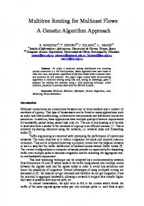
5 Computational results All the tests have been run on a 200 MHz PC Pentium MMX workstation. We note that ATM routing is done among nodes at the same hierarchical level, so the number of nodes has not to be too much large for realistic problems, [9]. The test networks were randomly generated and one additional real life network has been considered. The parameters are given bellow and are shown in figure 7: � Network A: 7 nodes and 18 links. Network B: 12 nodes and 46 links. � Network C: 15 nodes and 62 links. Network D: 18 nodes and 52 links. � Network E: Real life transport network with 9 nodes and 24.
Fig. 7. Test networks
We consider three different CBR demand scenarios representing three peak levels of demand. The lowest level (scenario I) is equivalent to a demand of 0.265 Mbps between every origin-destination pair, the medium level (scenario II) is equivalent to 0.8 Mbps and the highest level (scenario III) is equal to 1.55 Mbps. The five networks and the three demand levels imply a total amount of 15 different scenarios being analyzed. In table 1, we have used CLR parameter as an appropriated indication of the routing quality. Table 1. CLR and CPU time results. Network
-14
Demand scenario I II III I II III I II III I II III I II III
A
B
C
D
E
CLR (×10 ) 4.76 2.24 1.4 3.37 1.64 4 1.67×10 2.82 80.3 7 2.11×10 2.05 3 1.21×10 7 7.2×10 3.89 1.82 1.05
Average CPU time (seconds) 125.1
375.2
585.6
618.5
179.67
The table shows the increment of CLR when the number of nodes grows up because of the new connections with the rest of nodes. On the other hand, the different demand scenario affects directly to CLR excepting in network A case. For such case, the volume of traffic is very low and CLR does not grow up due to an upper increment of the total transmitted cells than the lost cells. The situation turns to critical only for very high density of nodes and traffic (cases C and D in scenario III). All of them are cases with a very large number of switches, even -14 higher than realistic problems. Figure 8 reveals CLR (×10 ) behavior versus the -14 number of nodes represented in a logarithmic scale: CLR* = ln (CLR×10 ). &/5 ��ORJDULWKPLF�VFDOH
���� ����
OQ�&/5 ��'HPDQG VFHQDULR�,,, OQ�&/5 ��'HPDQG VFHQDULR�,, OQ�&/5 ��'HPDQG VFHQDULR�,
���� ���� ���� ��� ���
�
�
��
��
��
QXPEHU�RI�QRGHV
Fig. 8. CLR in demand scenario I
Finally, with respect to the CPU time consumption we have to state that solutions are calculated in efficient time when we are dealing with real life dynamic routing in ATM networks, solving them in the order of seconds.
We have considered also for the real life network E the total number of lost cells for comparison with parameter CLR. Moreover, we have considered two additional demand scenarios: scenario IV with a demand of 3.11 Mbps and scenario V with a demand of 3.9 Mbps. The next table 2 summarizes the results. Table 2. CLR versus total lost cells for network E Network
E
Demand scenario I II III IV V
-6
Total lost cells (×10 ) 1.58 2.16 2.5 3 1.75×10 8 1.4×10
-14
CLR (×10 ) 3.89 1.82 1.05 2 3.68×10 4 2.25×10
The global losses increase in line with the traffic demand. While the network is not very saturated the total lost cells behavior shows bounded levels, however when the increment of traffic leads to the network congestion (critical point) the total lost cells grow strongly up. The figure 9 reveals the critical points for both -6 -14 total lost cells ×10 and CLR×10 parameters.
Fig. 9. Total lost cells and CLR as function of the demand scenario. Case network E
6 Conclusions In this paper, we have dealt with the routing problem in ATM networks considering matrix switches and queues at the end. We have presented a new model based on cell loss and a genetic algorithm to solve it with random parent selection, replacement based on fitness ranking, uniform crossover operators and entropy control. The fitness estimation is quickly evaluated by means of the individual chromosome encoding. The procedure showed an adequate behavior related to the cell loss rate (CLR), the total lost cells and the CPU time consumption. The tests were evaluated in both randomly generated and real life networks.
Appendix. Algorithm pseudo-code and parameters �� 5DQGRPO\�
JHQHUDWLRQ� RI� DQ� LQLWLDO SRSXODWLRQ� �� 3RSXODWLRQ�LQGLYLGXDOV�ILWQHVV�HYDOXDWLRQ�
VL]HG�1�
�� 'R� ZKLOH ^QXPEHU� RI� LWHUDWLRQV� �� 1B0$;` ^HQWURS\� !
6PLQLPXP` ���� ���� ���� ���� ����
&URVVRYHU�PXWDWLRQ�UDQGRPO\�VHOHFWLRQ� 3DUHQW�V �UDQGRPO\�VHOHFWLRQ� &DOFXODWH�WKH�QHZ�LQGLYLGXDO�ILWQHVV� &DOFXODWH� WKH� UHSODFHPHQW� SUREDELOLW\� RI WKH� LQGLYLGXDOV� DFFRUGLQJ� WR� WKH K\SHUJHRPHWULF�UXOH� 5HSODFH� WKH� VHOHFWHG� LQGLYLGXDO� E\ WKH� QHZ JHQHUDWHG�LQGLYLGXDO�
Table 3. Genetic algorithm parameters Population size, N Crossover probability, pc (mutation probability, 1-pc) Ranking based replacement probability, q Maximum number of iterations, N_ MAX Minimum entropy level, Sminimum Buffer size, b a
50 0.8 (0.2) a 0.2/0.7 50 0.25 10 cells
Replacement probability: 0.2 for first 20 iterations and 0.7 for following iterations
References 1.
Aboelela, E. and Douligeris, C. (1999) Fuzzy generalized network approach for solving an optimization model for routing in B-ISDN. Telecommunication Systems 12, 237-263. 2. Amiri, A. and Pirkul, H. (1999) Routing and capacity assignment in backbone communication networks under time varying traffic conditions. European Journal of Operational Research 117, 15-29. 3. Chou, L-D and Wu, J.L. (1998) Bandwidth allocation of virtual paths using neuralnetworks based genetic algorithms. IEE Proceedings on Communications Vol 145, No.1, 33-39. 4. Dahl, G., Martin, A. and Stoer, M. (1999) Routing through virtual paths in layered telecommunication networks. Operations Research 47, 693-702. 5. Ghanwani, A. (1998) Neural and delay based heuristics for the Steiner problem in networks. European Journal of Operational Research 108, 241-265. 6. Giroux, N. and Ganti, S. (1999) Quality of Service in ATM Networks (Prentice Hall). 7. Grefenstette, J.J. (1987) Incorporating problem-specific knowledge into genetic algorithms, in: L. Davis, ed., Genetic Algorithms and their Applications (Morgan Kaufmann, Los Angeles). 9. Lee, M-J and Yee, J-R (1994) An algorithm for optimal minimax routing in ATM networks. Annals of Operations Research 49, 185-206. 10. Medova, E. (1998) Chance-constrained stochastic programming for integrated services network management. Annals of Operations Research 81, 213-229. 11. Pitts, J.M. and Schormans, J.A. (1996) Introduction to ATM Design and Performance (Wiley&Sons). 12. Wang, C. and Weissler, P.N. (1995) The use of artificial neural networks for optimal message routing. IEEE Network, March-April,16-24.