A SAT-Based Routing Algorithm for Cross-Referencing ... - CiteSeerX

A SAT-Based Routing Algorithm for Cross-Referencing Biochips Ping-Hung Yuh∗ , Cliff Chiung-Yu Lin† , Tsung-Wei Huang‡ , Tsung-Yi Ho‡ , Chia-Lin Yang§ , Yao-Wen Chang†† ∗ Taiwan Semiconductor Manufacturing Company, Taiwan † Department of Electrical Engineering, Stanford University, Stanford, CA

‡ Department of Computer Science and Information Engineering, National Cheng Kung University, Tainan, Taiwan § Department of Computer Science and Information Engineering, National Taiwan University, Taipei, Taiwan

†† Department of Electrical Engineering and the Graduate Institute of Electronics Engineering, National Taiwan University, Taipei, Taiwan

Abstract—CAD problems for microfluidic biochips have recently gained much attention. One critical issue is the droplet routing problem. On cross-referencing biochips, the routing problem requires an efficient way to tackle the complexity of simultaneous droplet routing, scheduling and voltage assignment. In this paper, we present the first SAT based routing algorithm for droplet routing on cross-referencing biochips. The SAT-based technique solves a large problem size much more efficiently than a generic ILP formulation. We adopt a two-stage technique of global routing followed by detailed routing. In global routing, we iteratively route a set of nets that heavily interfere with each other. In detailed routing, we adopt a negotiation based routing algorithm and the droplet routing information obtained in the global routing stage is utilized for routing decision.. The experimental results demonstrate the efficiency and effectiveness of the proposed SAT-based routing algorithm on a set of practical bioassays.

I. I NTRODUCTION Due to the advances of microfabrication, there are many developments in the microfluidic technology [11]. Various conventional laboratory procedures can now be performed on microfluidic biochips with advantages such as the reduced sample/reagent volume, the shorter assay completion time, and the improved portability. As a result, microfluidic biochips are getting their popularity in molecular biology. Lately, the second-generation (digital) microfluidic biochips have been proposed [9]. On digital microfluidic biochips, droplets are controlled by the electrohydrodynamic forces generated by a 2D array of electrodes to achieve different droplet manipulations. Under the control of the electrodes, the droplets can move anywhere in the 2D array to perform the desired reactions. On a same biochip, the control sequences for the electrodes can be reconfigured for different bioassays. This is impossible on the first-generation (analog) microfluidic biochips, which manipulate continuous liquid using fixed micropumps. A typical digital microfluidic biochip contains a 2D array of cells for droplet movement. The simplest control scheme is to connect each electrode with a dedicated control pin, and thus each electrode can be individually controlled. In this paper, we refer to this type of biochips as direct-addressing biochips. Such a control scheme provides the highest flexibility for droplet movement. The only limit on the droplet movement is the fluidic constraint that prevents unexpected merging between distinct droplets. However, the number of control wires increases dramatically with the system complexity, and raises the production cost and control wiring complexity. Therefore, this architecture is only suitable for smallscale biochips [12]. To overcome this limitation, a new digital microfluidic biochip architecture has been proposed [5] recently. The architecture, referred to as cross-referencing biochips, uses a row/column addressing scheme for droplet movement, where a row/column of electrodes are connected to a control pin. In this way, the number of control pins can be greatly reduced. However, the major limitation of this architecture is the electrode interference problem, where a row/column of electrodes can potentially affect the movement of all droplets in the same row/column. This problem incurs a higher complexity for droplet movement than that of directaddressing biochips, and leads to performance degradation. Note that the

electrode interference problem is a global effect that affects all droplets in the same row/column. Therefore, we cannot naively extend the previous routing algorithms on the direct-addressing biochips [3], [4], [6], [10], [15] to solve the droplet routing problem on cross-referencing biochips. In this paper, we deal with the droplet routing problem on crossreferencing biochips. The main challenge is to ensure the correct droplet movement under the constraint imposed by the fluidic property of droplets, which prevents unexpected mixing among droplets, and the electrode activation problem, which prevents multiple droplets to move simultaneously. The goal of droplet routing is to minimize the maximum droplet transportation time for fast bioassay execution and better integrity.

A. Previous Work There are several works that handle the droplet routing problem in the literature [3], [4], [6], [10], [15], and all of them focus on direct-addressing biochips. However, due to the electrode interference problem, their method cannot be applied directly. Recently, several droplet manipulation methods have been proposed for cross-referencing biochips [6], [13], [14]. Griffith et al. [6] and Xu et al. [13] both proposed a graph-based method for droplet manipulation that based on given routing solutions for direct-addressing biochips. However, the initial routing solutions are not directly optimized for the cross-referencing architecture. Yuh et al. [14] proposed the first routing algorithm that directly targets at cross-referencing biochips. They proposed a progressive integer linear programming (ILP) based formulation that determines the droplet position progressively, one time step at a time. Therefore, their algorithm is not able to consider the routing information of other droplets when routing a droplet. This may lead to unnecessary droplet movement or detours, which increase the maximum droplet transportation time.

B. Our Contribution In this paper, we propose the first Boolean Satisfiability (SAT) based routing algorithm for the droplet routing on cross-referencing biochips. We adopt the SAT-based approach in our droplet routing algorithm regarding the nature of the problem and the recent advances of SAT solvers. The droplet routing problem, which will be formulated in Section III, involves only boolean variables in its constraints and is naturally more suitable to be solved as a boolean satisfiability problem. On the other hand, current state-of-art SAT solvers can solve problem instances with tens of thousands of variables and millions of clauses [2] and are much more efficient in handling large problem size when compared to ILP solvers. Furthermore, in order to utilize the routing information of other droplets when routing a droplet, we take a two-stage approach of global routing followed by detailed routing. In global routing, we iteratively identify a set of nets that heavily interfere with each other and find the optimal routing path and schedule the selected nets based on a SAT formulation. In detailed routing, we adopt a negotiation based method to simultaneously perform droplet routing, scheduling and voltage assignment with the aid of a 3D routing graph, which is used to offer higher flexibility. In this stage, the droplet routing information obtained in the global routing stage is utilized for routing decision. Our method

is also capable of handling multi-pin nets for efficient mix operations. Followings are the major contributions of this paper: • To reflect the nature of the problem, and to tackle the high routing complexity of cross-reference biochips, we propose the first SATbased routing algorithm for cross-referencing biochips. SAT-based techniques are more efficient than generic ILP formulations, therefore, they are more suitable of handling the complexity of the routing problem of cross-reference biochips, which requires simultaneous droplet routing, scheduling and voltage assignment. • Unlike [14] which does not have the routing information of other droplets when routing a droplet, our two-stage routing method allows the routing information obtained from the first-stage global routing to be utilized in detailed routing for routing decision. This avoids unnecessary droplet movement or detours thereby achieving better solution quality. • In detailed routing, we use a 3D routing graph, which allows the droplets to move back and forth in different time spans, and thus offers a higher flexibility for droplet movement than that in the 2D one, which implicitly implies that one droplet can visit one basic cell at most once. This flexibility is important for droplet routing on cross-referencing biochips due to the high complexity of droplet movement and the need for concessions between droplets. Experimental results demonstrate the effectiveness of the proposed routing scheme compared with previous indirect and direct approaches. For example, the proposed routing algorithm obtains smaller maximum droplet transportation time (19 cycles vs. 24 cycles) within reasonable CPU time for the in-vitro diagnostics, compared with the progressiveILP based routing scheme [14]. Our algorithm also obtains much better solution compared with indirect algorithms which require a directaddressing routing solution. The remainder of this paper is organized as follows. Section II describes the routing concerns on cross-referencing biochips and the problem formulation. Section III presents the proposed routing algorithm. Section IV shows our experimental results. Finally, concluding remarks are provided in Section V.

II. ROUTING ON C ROSS -R EFERENCING B IOCHIPS In this section, we first introduce the architecture of cross-referencing biochips. Then we describe the routing constraints for droplet routing on cross-referencing biochips. Finally, we present the problem formulation for the droplet routing problem.

A. Cross-Referencing Biochips

V

Y

Top electrode X

Figure 1.

Droplet

Bottom electrode

Top view of a cross-referencing biochip.

Figure 1 shows the top view of a cross-referencing biochip. A droplet is sandwiched by two plates. A set of orthogonal electrodes span a full row in the X -direction (the top plate) and a full column in the Y -direction (the bottom plate). Each set of the electrodes are assigned either a driving or reference voltage for droplet movement. A droplet can move to a basic cell (i.e., unit cells for droplet movement) only when the basic cell is “activated”; i.e., there is a voltage difference between the upper and lower electrodes. The advantage of this architecture is twofold [5]. First, we do not need a multi-layer architecture for electrodes. Second, the number of control wires for activating electrodes can be greatly reduced - it needs W + H

instead of W H control wires, where W (H ) is the width (height) of a biochip in terms of the number of electrodes in one dimension.

B. Routing Constraints (x+1, y+1, t+1)

(x, y, t)

t

y x

(x-1, y-1, t-1) Figure 2.

Illustration of the fluidic constraints.

There are two routing constraints in droplet routing: the fluidic constraint [10], [15] and the electrode constraint [14]. Both constraints are used to guarantee the correct droplet movement on cross-referencing biochips. The fluidic constraint says that if a droplet d uses a basic cell (x, y) at time t for routing, then no other droplets can use the eight neighboring cells of (x, y) from times t − 1 to time t + 1 for routing. Therefore, the fluidic constraints can be modeled as a 3D cube in the 3D space shown in Figure 2 [15], where the X and Y dimensions represent the biochip width and height, while the T dimension represents the droplet transportation time. Under this 3D models, to satisfy the fluidic constraints, no other droplet is allowed in the 3D cube defined by d. Cell (x+1, y) Cell that must be deactivated Cell that must be activated Droplet

Figure 3.

Cell (x, y)

The modeling of the electrode constraint.

When moving multiple droplets in a cross-referencing biochip, the assignments of voltage in rows/columns may cause unwanted or incorrect droplet movement, since a single row/column can be assigned only one voltage (high, low, or floating) at a time [13], [14]. This scenario is called electrode interference, and it must be avoided during droplet transportation. We refer to the restriction used to avoid the electrode interference as the electrode constraint. Figure 3 shows how we model the electrode constraint [14]. If a droplet d moves to cell (x + 1, y) from cell (x, y) at time t, then the eight neighboring cells of (x + 1, y) and (x, y); i.e., the green cells in Figure 3, must be deactivated, with only the cell (x + 1, y ) activated for droplet movement. If d stays at its original location instead, then the eight neighboring cells must be deactivated, but the underlying cell may or may not need to be activated. To make sure that these specific cells are deactivated, restrictions must be applied on the electrodes on the same row/column.

C. Problem Formulation In this paper, we deal with the droplet routing problem on crossreferencing biochips. We use the same partitioning method in [10], [15], in which the bioassay reactions are divided into a set of 2D planes based on the time they are scheduled. Since the reactions on different planes happens in different time slots, the routing problem can be solved independently. Thus, in this subsection, we focus our problem formulation on the subproblem on one 2D plane at a time. Several issues should be considered about the droplet transportation. Besides the fluidic and electrode constraints, the problem formulation takes obstacles and 3-pin nets into account. When we are routing the droplets on a 2D plane, the modules being used for reactions and the

TABLE I

T HE NOTATIONS USED IN OUR ALGORITHM . N (N 0 ) D dij ˆ C (C) (x, y, t) Uf (x, y, t) Ue (x0 y 0 , x, y, t)

set of all (3-pin) nets set of droplets j-th droplet of net ni ; j = {1, 2} set of basic (global) cells a basic cell (x, y) at time t 0 0 0 s{(x , y , t )||x − x0 | ≤ 1, |y − y 0 | ≤ 1, |t − t0 | ≤ 1} set of eight neighboring basic cells of (x0 , y 0 ) and (x, y), except (x, y), at time t a global cell (xg , yg ) at time tg global cell location of the source of dij global cell location of the sink of net ni set of global cells with the same xor y-coordinate as (xg , yg ) except (xg , yg ) set of basic cells with the same xor y-coordinate as (x, y) except (x, y) four adjacent global cells of (xg , yg ) and (xg , yg ) itself a 0-1 variable to represent that every droplet reaches its sink at time tg a 0-1 variable to represent the congestion of (xg , yg ) at time tg is greater than or equal to k a 0-1 variable to represent that at least one variable c˜(xg , yg , tg , k) is one a 0-1 variable to represent that droplet dij locates at the global cell (xg , yg ) at time tg a 0-1 variable to represent that the two droplets of net ni are merged at (xg , yg ) at time tg . a 0-1 variable to represent that the droplet of two nets ni and ni0 are in their common sink at time tg base cost for the node vx,y,t in detailed routing fluidic penalty for node vx,y,t in detailed routing electrode penalty for node vx,y,t in detailed routing activation penalty for node vx,y,t in detailed routing deactivation penalty for node vx,y,t in detailed routing

(xg , yg , tg ) i,j (si,j g,x , sg,y ) (tˆig,x , tˆig,y ) g Ex /Eyg b Ex /Eyb

˜ g , yg ) A(x a(tg ) c˜(xg , yg , tg , k) c˜M k pij (xg , yg , tg ) i

m (xg , yg , tg ) t˜(i, i0 , tg ) ˆ B(x, y, t) Fˆ (x, y, t) ˆ 0 , y 0 , x, y, t) E(x ˆ A(x, y, t) ˆ D(x, y, t)

surrounding segregation cells are considered as obstacles. And 3-pin nets are necessary for practical bioassays since two droplets need to be merged during their transportation for efficient mix operations [10]. Therefore, we formulate the droplet routing problem as follows: Input: A list of m nets N = {n1 , n2 , . . . , nm }, where each net ni can be a 2-pin net (one droplet) or a 3-pin net (two droplets), and the locations of pins and obstacles. Objective: Route all droplets from their source pins to their target pins while minimizing the maximum time to route all droplets. Constraint: Both fluidic and electrode constraints must be satisfied, and the droplet routing should not step on the obstacles.

III. B IOCHIP ROUTING A LGORITHM Obstacles introduced by d 2 Droplet d1

Droplet d 2

t1 Sink of d1

t2

t1

t2

t1 (a)

Figure 4.

t2 Sink of d 2

(b)

The motivation. Droplet d1 moves one cell left (a) or stay at its original

location (b).

The proposed biochip routing algorithm is a two-stage technique of global routing followed by detailed routing. There are two main advantages of the two-stage approach. First, a subset of the nets which heavily interfere with each other are first routed in the global routing phase. With the reduced problem size, the optimal routing solution could be found through a SAT formulation. Second, the global routing information could be utilized in detailed routing for better routing decision.

Unlike the previous works that route the droplets independently and incrementally, we maintain the routing information of all droplets during the whole process. Figure 4 illustrates the importance of considering the routing information of other droplets when routing a droplet. Note that droplet d2 is considered as a 3 × 3 obstacle when determining the routing cost of d1 due to the fluidic constraints. Previous works determine droplets’ movement cost based only on the current positions of all droplets. Therefore, d1 may move one cell left due to shorter distance to its sink and less routing congestion, as shown in Figure 4 (a). However, if the routing path of d2 is known, then d1 may stall, resulting with lesser cycles to move to its sink, as shown in Figure 4 (b). In other words, the absence of routing path information of other droplets may introduce unnecessary detours, which increases the droplet transportation time. Therefore, it is important to know the routing path of all other droplets while routing a droplet. In this section, we first introduce the overview of the proposed algorithm. We then detail the global and detailed routing algorithms. The notations used in our algorithm are given in Table I.

A. Routing Algorithm Overview Inputs: 1. Net list 2. Pin locations

3. Obstacle locations

Net criticality determination Global Routing

Detailed Routing 3D routing (routing and scheduling) and voltage assignment

Net selection ILP formulation construction

Yes

Nets routing All nets are routed?

No

Failed nets reroute Refinement

Yes

Figure 5.

Routing success or iteration limit is reached? No

Termination

The routing algorithm overview.

Figure 5 shows the overview of the proposed routing algorithm. There are three phases in our algorithm: (1) net criticality calculation, (2) SATbased global routing formulation, and (3) detailed routing based on a negotiation based routing scheme. In net criticality calculation, we estimate the level of interference between net pairs and the criticality of each net. This information will be used in both global routing and detailed routing. In global routing, the goal is to determine a rough routing path and schedule of each droplet and to minimize the interference among droplets. We divide a biochip into a set of global cells. We first select a set of nets that heavily interfere with each other. Based on these global cells, we construct the SAT formulation and then transform it into an equivalent conjunctive normal form (CNF) for routing, where CNF is the conjunction of disjunctions of boolean variables. In detailed routing, the goal is to simultaneously perform routing and scheduling and voltage assignment based on the result of global routing. A 3D routing graph is used, where each node represents a basic cell at a time step. Performing routing and scheduling is equivalent to finding a routing tree on the 3D routing graph. A post-step refinement is performed after finding a feasible solution. The whole algorithm terminates when there is no further improvement or no feasible solution can be found within a specified maximum number of iterations.

B. Net Criticality Calculation We say a net ni is critical if many other nets interfere with ni . Let ˜ i0 ) denote the level of interference between two nets ni and ni0 . I(i,

˜ i0 ) is defined in the following equation: I(i,

X

˜ i0 ) = I(i,

ˆ ,(x0 ,y 0 ,t0 )∈U (x,y,t) (x,y,t)∈U i f

u ˆi0 (x0 , y 0 , t0 ) + ˆi ||U ˆ 0| |U i

0

X ˆ ,(x0 ,y 0 )∈E b ∪E b ∪{(x,y)} (x,y,t)∈U i x y

u ˆi0 (x , y 0 , t) , ˆi ||U ˆ 0| |U

(1)

i

ˆi is the set of (x, y, t) that can be used by di , j = 1, 2, for routing where U j 0 and u ˆi0 (x0 , y 0 , t0 ) is one if dij , j = 1, 2, can use (x0 , y 0 , t0 ) for routing; otherwise, u ˆi0 (x0 , y 0 , t0 ) is zero. The first term represents the possibility of violating the fluidic constraints while the second term represents the ˜ i0 ) is large, then the possibility of violating the electrode constraint. If I(i, routing solution of ni is very likely to be affected by the routing solution of ni0 . Finally, we define the criticality of ni , denoted as crit(i), as

X

crit(i) =

I(i, i0 ).

(2)

∀i0 6=i,ni0 ∈N

C. Global Routing

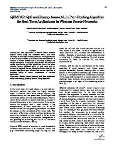
global cell. Thus, the two cases must be allowed in the global routing formulation. Due to obstacles, droplets may not move from a global cell to another global cell. This restriction must be modeled in our SAT formulation. We say that three adjacent global cells {(xg1 , yg1 ), (xg2 , yg2 ), (xg3 , yg3 )} as a turn. Obstacles may prevent a droplet from moving from a global cell (xg1 , yg1 ) to another global cell (xg2 , yg2 ) via cell (xg3 , yg3 ). For example, as shown in Figure 6, droplets are not allowed to move from (0, 3) to (1, 2) via (1, 3). If no droplets can move via a turn, we say that this turn is prohibited. The constraint that uses no prohibited turns is called turn prohibition constraint and must be satisfied in global routing. A simple maze routing algorithm can be used to determine all prohibited turns. The sources (sinks) of maze routing are the basic cells along the boundary of (xg1 , yg1) ((xg3 , yg3 )). Only basic cells that are in the global cell (xg2 , yg2 ) (and sources/sinks) can be used for routing. If there is a path from a source to a sink, then this turn is not a prohibited turn. For example, the turn {(0, 3), (1, 3), (1, 2)} shown in Figure 6 is a prohibited turn. In the following subsections, we first introduce how to construct the SAT formulation.

Obstacle Sources for maze routing Sinks for maze routing

(0,3)

(1,3)

(2,3)

(3,3)

(0,2)

(1,2)

(2,2)

(3,2)

(0,1)

(1,1)

(2,1)

(3,1)

(0,0)

(1,0)

(2,0)

(3,0)

Net 3

(0,3)

(1,3)

(2,3)

(3,3)

(2,2)

(3,2)

Net 4

(0,2)

Net 1

(0,1)

(1,1)

(2,1)

(3,1)

(0,0)

(1,0)

(2,0)

(3,0)

Net 2

Figure 6. The illustration of a biochip being partitioned into a set of global cells and

Figure 7.

The illustration of the congestion in global routing.

the determination of a prohibited turn.

The purpose of global routing is to determine a rough routing path and schedule for droplets and to minimize the interference among droplets. We decompose the global routing problem into a set of subproblems by selecting a set of nets that heavily interfere with each other. In this subsection, we first explain how the net selection is done. Then we present the SAT formulation for the global routing problem on the selected nets. 1) Net Selection: We use a heuristic for net selection. We first select na and nb with the maximum interference value, denoted as I M , into a set Ng . Then we iteratively add a net nc into Ng if it satisfies the following equation: 0.5 ×

X

Objective Function: The goal of the global routing is to minimize the maximum droplet transportation time and the interference among droplets by minimizing the maximum congestion of all global cells. The congestion of a global cell is defined as the number of droplets that may affect the movement of droplets in it. Note that a droplet introduces one unit of congestion to all cells (x0g , yg0 ) ∈ Exg ∪ Eyg at time t if (xg , yg , tg ) is used for routing at time t, as shown in Figure 7. Note that if there are no droplets in a global cell, we do count for the congestion of it. Therefore, the objective function is defined by the following equation:

β I(a, c) + 0.5 × max I(a, c) ≥ α × I

M

,

(3)

na ∈Ng

X

tg (a(tg ) − a(tg − 1)) + γ

1≤tg