314
ACTA ELECTROTEHNICA
A Hopfield Solution to Economic Dispatch Problem with Transmission Losses F. BENHAMIDA ABSTRACT: This paper concentrates on the solution of economic dispatch (ED) problem of thermal generators with transmission losses using a fast-solver which is a Hopfield Neural Network (HNN) algorithm. A direct computation Hopfield neural network method has been developed and used for solving problem, which employs a linear input-output model for the neurons. Formulations for solving the ED problem are explored. Through the application of these formulations, direct computation instead of iterations for solving the problem becomes possible. Unlike the usual Hopfield methods, which select the weighting factors of the energy function by trials, the proposed method determines the corresponding factors by calculations. The effectiveness of the developed method is identified through its application to the 15-unit system. Computational results manifest that the method has a lot of excellent performances. KEYWORDS: Economic Dispatch, Hopfield model, Energy function, Linear input-output model.
1. INTRODUCTION The economic dispatch problem (EDP) objective is to minimize production cost while satisfying demand and working area constraints for a given combination of active units. Aside from using the solutions of the EDP (combination of units with the least production cost) for its own merits in system operation, they are used to guide the solution method that solves the combinatorial part of the unit commitment problem. When the combinatorial part of the unit commitment problem is solved, solutions from the EDP are used to estimate the quality of different unit combinations. In this chapter the construction and implementation of an exact method using the Hopfield Neural Network that solves both the economic dispatch problem is presented. The performance of such method with respect to time and solution quality is a crucial part in the solution process of solving the unit commitment problem. The use of the Hopfield neural network methods to solve the EDP is therefore justifiable if the method produces
© 2008 – Mediamira Science Publisher. All rights reserved.
optimal solutions and outperforms nearoptimal solver with respect to computation time. 2. PROBLEM FORMULATION Economic dispatch (ED) is defined as the process of allocating generation levels to the thermal generating units in service within the power system, so that the system load is supplied entirely and most economically [1] and [2]. The objective of the ED problem is to calculate, for a single period of time, the output power of every generating unit so that all demands are satisfied at minimum cost, while satisfying different technical constraints of the network and the generators. The problem can be modeled by a system which consists of N generating units connected to a single bus-bar serving an electrical load D. The input to each unit shown as Fi, represents the generation cost of the unit. The output of each unit Pi is the electrical power generated by that particular unit. The total cost of the system is the sum of the costs of each of the individual units. The essential constraint on
Volume 49, Number 3, 2008
the operation is that the sum of the output powers must equal the load demand. The standard ED problem can be described mathematically as an objective with two constraints as: N
min FT = ∑ Fi (Pi )
(1)
i =1
Subject to the following constraints: N
∑P = D + L i =1
i
(2)
Pi min ≤ Pi ≤ Pi max Where Pi : Real power output of i-th generator (MW); FT : Total Operating cost ($ /h); Fi ( Pi ) : Operating cost of unit i ($ /h); D : Total demand (MW); L : Transmission losses (MW); Pi min , Pi max : Operating power limits of unit i (MW); N: total number of units in service.
The fuel cost function or input-output characteristic of the generator may be obtained from design calculations or from heat rate tests. Many different formats are used to represent this characteristic. The data obtained from heat rate tests or from the plant design engineers may be fitted by a polynomial curve. It is usual that, quadratic characteristic is fit to these data. A series of straight-line segments may also be used to represent the input-output characteristic [1]. The fuel cost function of a generator that usually used in power system operation and control problem is represented with a second-order polynomial. (3) Fi(Pi) = ai + bi Pi + ci Pi 2 Where, ai, bi and ci are the cost coefficients (non-negative constants) of the i th generating unit. For some generators such as large steam turbine generators, however, the input-output characteristic is not always as smooth as (2.3). Large steam turbine generators will have a number of steam admission valves that are opened in sequence to obtain ever-increasing
315
output of the unit [3], [4]. The fuel cost function in this case can be expressed as: Fi ( Pi ) = ai + bi Pi + ci Pi 2 + ei sin( f i ( Pi min − Pi )) (4) Where ei and fi are non-negative constants. Alternatively, fuel cost functions may be represented by piecewise-linear cost functions, such as the Willans line [5] described by: (5) Fi(Pi) = incikPi+nlik k=1,2,…,3 Where: incik: incremental cost of segment k of unit i ($/MWh), k = 1, 2, and 3; k nli : no-load cost of segment k of unit i ($/h), k = 1, 2, and 3; Eq(5) can be written in more detail as: (6) Fi(Pi)=inci1Pi+nli1, Pimin≤Pi θ i The continuous or deterministic model of the Hopfield Neural Network is based on continuous variables. The output variable of neuron i has the range Vi0 < Vi < Vi1 and the input-output function is a continuous and monotonically increasing function of the input Ui to neuron i. The model is a mutual coupling neural network and of non-hierarchical structure. The dynamic characteristic of each neuron can be described by the following differential equation [9] and [10]. N dU i T ijV j + I i = ∑ dt , j =1
(13)
Where Tii is the self-connection conductance of neuron i. The output of neuron is given by Vi = fi (Ui) (14) Where fi (Ui) is the input-output function of the neuron i. The energy function of the continuous Hopfield model can be defined as: E =−
N 1 N N T V V − I iV i ∑∑ ij i j ∑ 2 i =1 j =1 i =1
(15)
The time derivative of the energy function can be proved to be negative [11]. Therefore, in the computation process the model state always moves in such a way that the energy function gradually reduces and converges to a minimum. This model is suitable for economic dispatch, while the discrete model is suitable for unit commitment. 3.2. Mapping Economic Dispatch to Hopfield Neural Network
The Hopfield model of neural networks [12] has been employed to solve the ED problem for units having continuous or piece wise quadratic fuel cost function [9] and [13], and even for units having prohibited zones
Volume 49, Number 3, 2008
constraint [14] and [15]. The conventional Hopfield model belongs to the kind of continuous and deterministic model, and the input-output relationship for its neurons is described by a modified sigmoidal function. Due to the use of sigmoidal function in the conventional Hopfield model, in solving the ED problems, a method involving numerical iterations is inevitably applied; this numerical iteration method often suffers from large amount of computational requirements. Adopting a modified sigmoidal function causes two other problems. The first, it incurs unreasonable or incorrect generation dispatch, which is attributable to the serious saturation phenomena existing in the input-output relationship represented by the sigmoidal function. The second; it is troublesome to select shape constant of the sigmoidal function. A fast Hopfield Neural Network method to solve the ED problem is presented. The method employs a linear input-output model for the neurons. Formulations for solving the ED problem are explored. Through the application of these formulations, direct computation instead of iterations for solving the problem becomes possible. Not like the usual Hopfield methods, which select the weighting factors of the energy function by trials, this method determines the corresponding factors by calculation. The adoption of a linear model describing the input-output relationship of the neuron has resulted in the avoidance of the aforementioned problems. To solve the ED problem using the Hopfield method, energy function including both power mismatch, Pm and total fuel cost F is defined as follows: 2
N A⎛ ⎞ E = ⎜ ( D + L ) − ∑ Pi ⎟ + ... 2⎝ i =1 ⎠
B N (16) ∑ ( ai + bi Pi + ci Pi 2 ) 2 i =1 A B = Pm 2 + FT 2 2 A and B introduce the relative importance of their respective associated terms.
317
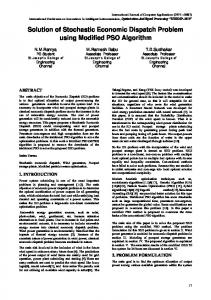
Comparing eq(15) with eq(16), we get: Tii = − A − B . ci (17) Tij = − A (18) Ii = A (D + L) – B (bi /2) (19) At this stage the transmission losses L can be neglected and reconsidered later in section 4. Substituting eq(17), eq(18) and eq(19) into (13), the dynamic equation becomes, dUi B ⎛ dF ⎞ (20) = APm − ⎜⎜ i ⎟⎟ dt ' 2 ⎝ dPi ⎠ Application of the conventional Hopfield method to the ED problem, the power output value can be represented by the output Vi of neuron i using a modified sigmoidal function, described as follows [13] and [14]: Pi = f i (U i ) ⎛ U ⎞ (21) 1 max Pi − Pi min ) ⎜1 + tanh i ⎟ ( 2 u0 ⎠ ⎝ Where u0 is the shape constant of the sigmoidal function. To avoid the problems resulting from curve saturation, a linear model shown in figure 1 is used to describe the input-output relationship for the neuron instead of the sigmoidal function. Linear transfer function of the ith neuron is defined as follows: = Pi min +
Pi = fi (U i ) ⎧ U i − U min max min min U min ≤ U i ≤ U max ⎪U − U .( Pi − Pi ) + Pi max min ⎪ ⎪ U i ≥ U max = ⎨ Pi max ⎪ min U i ≤ U min ⎪ Pi ⎪⎩
(22) Pi max
...
Pi min
Umin
Umax
Fig. 1. The proposed linear input-output function.
Substituting eq(22) in eq(20) the dynamic equation becomes:
318
ACTA ELECTROTEHNICA
dU i B = APm − ( bi + 2ci ( K 1i U i + K 2i ) ) (23) , 2 dt Pi max − Pi min , K 2i = Pi min − K1iU min . U max − U min Solving (23) the neuron’s input function, , Ui( t ) is obtained as: With K1i =
, ⎛ K ⎞ K U i (t , ) = ⎜ U i (0) + 4i ⎟ e K3it − 4i K 3i ⎠ K 3i ⎝ With K 3i = − Bci K 1i
B bi − Bci K 2i 2 From eq(22), the neuron’s function, Pi( t , ), is obtained as: K 4i = APm −
Pi (t , ) =
(24)
4. INCLUSION OF TRANSMISSION LOSSES IN A HYBRID ALGORITHM
(25)
The transmission losses L can be either given from a load flow study or approximated by traditional representation using B coefficients:
(26) output
N
N
N
L = ∑∑ PB i cij Pj + ∑ B0 i Pi + B00 i =1 j =1
2K AB Pm − bi + .... 2ci
(32)
i=1
L = P Bc PT + B0 PT + B00 (Matrix form) (33)
⎛ ⎛ 2K P − b ⎞ ⎞ ... ⎜⎜ K1iUi (0) + K2i − ⎜ AB m i ⎟ ⎟⎟ eK3it ' 2ci ⎝ ⎠⎠ ⎝
(27)
A . B The second term in eq(27) decays exponentially, finally becomes vanishingly small and eventually setting t , = ∞ , eq(27) gives, 2 K AB Pm − bi P i (∞ ) = (28) 2ci Where KAB =
P i (∞) represents the optimal Here generation level of unit i, which is the required solution. Back substituting of eq(28) in eq (27), a more simple formula for the generation function is given as: Pi (t , ) = Pi (∞) + ( P i (0) − P i (∞) ) e K3it
N ⎛ ⎛ 1 ⎞⎞ 1 K + ⎜ ⎟ ⎟ (31) AB ∑ ⎜ c = 1 i i ⎝ ⎠ ⎝ ⎠ Equations (28) through eq(31) constitute the Hopfield model for the economic dispatch problem. A non iterative direct computation process is, therefore, possible.
⎛ 1 N b⎞ Pm = ⎜ D + ∑ i ⎟ 2 i =1 ci ⎠ ⎝
,
(29)
Where P i (0) is obtained from eq(27) by letting t’= 0, to give: Pi (0) = K 2i + K1iU i (0) (30) It should be noted here that t’ is not representing real time, it is a dimensionless variable. Using the power mismatch definition and eq(28) we obtain:
Where P: vector of generator loading ( P1 , P2 ,… , PN ) , Bc: loss-coefficient matrix, B0: loss-coefficient vector, B00: loss constant. A Bisection solution method for solving the economic dispatch including transmission losses combined to the Hopfield Neural Network is presented in the following steps: Step1: initialization of the interval search [D3 D1]. ε : a pre-specified tolerance. Initialize the iteration counter k =1. D3 k = D ; D1 k = D3 k + 0.1 * D3 k ; D2 k = D3 k + (D1 k-D3 k) / 2 ; Step2: Determine the optimal generators’ power outputs Pi , i = 1,..., N using the Hopfield Neural Network algorithm, by neglecting losses and setting the power demand as D k = D2 k ; Step3: Calculate the transmission losses Lk for the current iteration k using eq(32); Step 4: if D1k -D3k < ε , stop otherwise go to step 5; Step5: if D2k-Lk < D, update D3 and D2 for the next iteration as follows: D3k+1 = D2k D2k+1=D2k + ( D1k - D2k ) /2;
Volume 49, Number 3, 2008
Replace k by k+1 and go to step 2; Step 6: if D2k-Lk > D, update D1 and D2 for the next iteration as follows: D1k+1=D2k D2k+1=D2k - ( D2k – D3k ) /2; Replace k by k+1 and go to step 2.
319
constraints must be not violated. The system consists of 15-units where data is given in table1. For comparison the case of a load demand of 2650 MW is considered as in [16]. The total operating cost of the system is represented by the following polynomial, N
FT = ∑ Fi ( Pi ) =
5. RESULTS AND DISCUSSION
i =1
N
∑(a + b P + c P ) 2
i =1
i
i i
i i
(34)
Where the polynomial coefficients are listed in table 1 along with generator minimum and maximum operating limits.
To demonstrate the performance of the Hopfield based ED solver, a 15-unit test system [16] is used, where the convergence criteria considered here is the unit generation
Table 1. Input data of 15-unit system and the computational results. Unit 1 2 3 4 5 6 7 8 9 10 11 12 13 14 15
Pi min (MW) 150 150 20 20 150 135 135 60 25 20 20 20 25 15 15
Pi max (MW) 455 455 130 130 470 460 465 300 162 160 80 80 85 55 55
b c a $/hr $/MWhr $/MW2hr 671.03 10.07 0.000299 574.54 10.22 0.000183 374.59 8.8 0.001126 374.59 8.8 0.001126 461.37 10.4 0.000205 630.14 10.1 0.000301 548.2 9.87 0.000364 227.09 11.5 0.000338 173.72 11.21 0.000607 175.95 10.72 0.001203 186.86 11.21 0.003586 230.27 9.9 0.005513 225.28 13.12 0.000371 309.03 12.12 0.001929 323.79 12.41 0.004447 Transmission losses L (MW) Total production power generation (MW) Total production cost FT ($)
Pi (MW) 455 455 130 130 317.8331 460. 465 60 25 20 20 57.1659 25 15 15 0 2650 32542.30
Pi (MW) 455 455 130 130 348.7724 460. 465 60 25 20 20 58.3164 25 15 15 32.1138 2682.0898 32880.42
The loss coefficients matrix Bc 10−2 , vector B0 and constant B00 are shown in the following: 0.0014 0.0012
0.0012 0.0015
0.0007 0.0013
-0.0001 0.0000
-0.0003 -0.0005
-0.0001 -0.0002
-0.0001 0.0000
-0.0001 0.0001
-0.0003 -0.0002
-0.0005 -0.0004
-0.0003 -0.0001
-0.0002 -0.0000
0.0004 0.0004
0.0003 0.0010
-0.0001 -0.0002
0.0007
0.0013
0.0076
-0.0001
-0.0013
-0.0009
-0.0001
0.0000
-0.0008
-0.0012
-0.0017
-0.0000
-0.0026
0.0111
-0.0028
-0.0001
0.0000
-0.0001
0.0034
-0.0007
-0.0004
0.0011
0.0050
0.0029
0.0032
-0.0011
-0.0000
0.0001
0.0001
-0.0026
-0.0003
-0.0005
-0.0013
-0.0007
0.0090
0.0014
-0.0003
-0.0012
-0.0010
-0.0013
0.0007
-0.0002
-0.0002
-0.0024
-0.0003
-0.0001
-0.0002
-0.0009
0.0004
0.0014
0.0016
-0.0000
-0.0006
-0.0005
-0.0008
0.0011
-0.0001
-0.0002
-0.0017
0.0003
-0.0001
0.0000
-0.0001
0.0011
-0.0003
-0.0000
0.0015
0.0017
0.0015
0.0009
-0.0005
0.0007
-0.0000
-0.0002
-0.0008
-0.0001
0.0001
0.0000
0.0050
-0.0012
-0.0006
0.0017
0.0168
0.0082
0.0079
-0.0023
-0.0036
0.0001
0.0005
-0.0078
-0.0003
-0.0002
-0.0008
0.0029
-0.0010
-0.0005
0.0015
0.0082
0.0129
0.0116
-0.0021
-0.0025
0.0007
-0.0012
-0.0072
-0.0005
-0.0004
-0.0012
0.0032
-0.0013
-0.0008
0.0009
0.0079
0.0116
0.0200
-0.0027
-0.0034
0.0009
-0.0011
-0.0088
-0.0003
-0.0004
-0.0017
-0.0011
0.0007
0.0011
-0.0005
-0.0023
-0.0021
-0.0027
0.0140
0.0001
0.0004
-0.0038
0.0168
-0.0002
-0.0000
-0.0000
-0.0000
-0.0002
-0.0001
0.0007
-0.0036
-0.0025
-0.0034
0.0001
0.0054
-0.0001
-0.0004
0.0028
0.0004
0.0004
-0.0026
0.0001
-0.0002
-0.0002
-0.0000
0.0001
0.0007
0.0009
0.0004
0.0001
0.0103
-0.0101
0.0028
0.0003
0.0010
0.0111
0.0001
-0.0024
-0.0017
-0.0002
0.0005
-0.0012
-0.0011
-0.0038
-0.0004
-0.0101
0.0578
-0.0094
-0.0001
-0.0002
-0.0028
-0.0026
-0.0003
0.0003
-0.0008
-0.0078
-0.0072
-0.0088
0.0168
0.0028
0.0028
-0.0094
0.1283
B0 i = [ -0.000l -0.0002 0.0028 -0.0001 0.0001 -0.0003 -0.0002 -0.0002 0.0006 0.0039 -0.0017 -0.0000 -0.0032 0.0067 0.0064] B00 = 0.0055.
320
ACTA ELECTROTEHNICA
The seventh column of table 1 shows the optimal generators’ power outputs when the transmission losses is neglected. Total production cost is $ 32542.30. The problem was carried out on Pentium M 1.73 MHz using the presented Hopfield method with Umin = 0.5, Umax = 0.5 and Pm = 0.001. The computation time was about 0.14 s. The same test system was solved in [16], the total production cost is obtained as $ 32549.8. It can be seen that the presented Hopfield approach could provide a better solution within a much shorter time.
The last column of table 1 shows the optimal generators’ power outputs when the transmission losses is taken into account. The pre-specified tolerance was taken as 0.001. Total production cost is $ 32880.42, and the transmission losses equal to 32.1138 MW. The computation time was about 0.51 s for 21 iterations. The iterative search results using the HNN method for iterations (1 to 11 and last iteration 21) are given in table 2.
Table 2. Iterative search results using HNN method for the 15-unit system.
Transmission losses Lk (MW) Total production power generation D2 k(MW) D2k-Lk (MW) Total production cost FT k($) Pi (k =6) (MW) 455 455 130 130 345.7783 460 465 60 25 20 20 58.2051 25 15
Pi (k =7) (MW) 455 455 130 130 347.7744 460 465 60 25 20 20 58.2793 25 15
Pi (k =8) (MW) 455 455 130 130 348.2734 460 465 60 25 20 20 58.2979 25 15
Pi (k =1) (MW) 455 455 130 130 445.5827 460 465 60 25 20 20 61.9163 25 15 15 38.50 2782.50 2744.00 33941.04
Pi (k =2) (MW) 455 455 130 130 381.7079 460 465 60 25 20 20 59.5411 25 15 15 34.097 2716.25 2682.15 3240.80
Pi (k =9) (MW) 455 455 130 130 348.52 460 465 60 25 20 20 58.3071 25 15
Pi (k =3) (MW) 455 455 130 130 349.7705 460 465 60 25 20 20 58.3535 25 15 15 32.17 2683.125 2650.95 32891.33
Pi (k =10) (MW) 455 455 130 130 348.64 460 465 60 25 20 20 58.3118 25 15
Pi (k =4) (MW) 455 455 130 130 333.8018 460 465 60 25 20 20 57.76 25 15 15 31.27 2666.562 2635.28 32716.76
Pi (k =11) (MW) 455 455 130 130 348.71 460 465 60 25 20 20 58.3141 25 15
Pi (k =5) (MW) 455 455 130 130 341.7861 460 465 60 25 20 20 58.0566 25 15 15 31.71 2674.843 2643.12 32804.036
Pi (k =21) (MW) 455 455 130 130 348.7724 460. 465 60 25 20 20 58.3164 25 15
Volume 49, Number 3, 2008
15 31.94 2678.9844 2647.041 32847.6826
15 32.056 2681.055 2648.9979 32869.5082
15 32.085 2681.5723 2649.487 32874.9649
15 32.01 2681.83 2649.73 32877.693
6. CONCLUSION
A Hopfield neural network method combined to bisection has been developed for ED problems solution with transmission losses. This fast-computation solver, overcomes the drawbacks of the conventional segmoidal function by adopting a linear input/output transfer function, resulting in a superior Hopfield neural network as one calculation process is required (i.e. No iterations). This led to a very short computing time and suitability for on-line usage. The proposed method is relatively simple, straightforward, efficient, easy to apply and requires no training. Its connective conductances and external input can be determined directly by employing system data. REFERENCES 1. A.J. Wood and B.F. Wollenberg, “Power Generation, Operation and Control,” New York, John Wiley and Sons, 1984. 2. B.H. Chowdhury and S. Rahman, “A Review Of Recent Advances In Economic Dispatch,” IEEE Transactions on Power Systems, Vol. 5, No. 4, Nov. 1990, pp. 1248-1259. 3. P. Attaviriyanupap, “The Applications of Evolutionary Programming-based Optimization Method to Power System Generation before and after Deregulation,” PHD thesis, Systems and Information Engineering, Hokkaido University, Dec. 2002 4. T.A.A. Victoire, A.E. Jeyakumar, “A modified hybrid EP–SQP approach for dynamic dispatch with valve-point effect,” Electrical Power and Energy Systems, Vol. 27, Nov. 2005, pp. 594-601. 5. C.j.S. Shan., “Development of a Profit Maximization Unit Commitment Problem,” Msc Thesis University of Manchester, Institute of science and technology, Sept. 2000. 6. J.O. Kim, D.J. Shin, J.N. Park and C. Singh, “Atavistic Genetic Algorithm for Economic Dispatch with Valve Point Effect,” Electric Power Systems Research, Vol. 62, No. 3, Jul. 2002, pp. 201-207. 7. M. Aganagic and S. Mokhtari, “Security Constrained Economic Dispatch Using Nonlinear
15 32.106 2681.96 2649.85 32879.057
321
15 32.11 2682.025 2649.915 32879.7396
15 32.1138 2682.0898 2649.975 32880.42
Dantzig-Wolfe IEEE Decomposition,” Transactions on Power Systems, Vol. 12, No. 1, Feb. 1991, pp. 105-112. 8. Y.S. Kim, I.K. Eoz and J.H. Park. “Economic Power Dispatch for Piecewise Quadratic Cost Function using Neural Network,” IEE International Conference on Advances in Power System Control, Operation and Management, Hong Kong, Nov. 1991. 9. C.T. Su and G.J. Chiou, “Hopfield Neural Network Method for Economic Load Dispatch of Power System,” Proceedings of the IASTED international Conference on Modeling and Simulation, Colombo, Sri Lanka , Jul. 1995, pp. 209-212. 10. G.G. Lendaris, K. Mathia, and R. Saeks, “Linear Hopfield Networks and Constrained Optimization,” Accurate Automation Corp. of Chattanooga, submitted for Government Review, Sept. 1994. 11. J.M. Zurada, “Introduction to Artificial Neural Network Systems,” Mumbai, Jaiko Publishing house, 1996. 12. J.J. Hopfield and D.W. Tank, “Neural Computation of Decisions in Optimization Problems,” Biological Cybernetics, Vol. 52, 1985, pp. 141-152. 13. S. Matsuda and Y. Akimoto, “The Representation of Large Numbers in Neural Networks and its Application to Economical Load Dispatching of Electric Power,” Proceedings of the International Conference on Neural Networks (ICNN), Vol. 1, 1989, pp. 587-592. 14. J.H. Park and al., “Economic Load Dispatch for Piecewise Quadratic Cost Function using Hopfield Neural Network,” IEEE Transactions on Power Systems, Vol. 8, No.3, 1993, pp. 1030-1038. 15. C.T. Su and G.J. Chiou, “A Hopfield Neural Network Approach to Economic Dispatch with Prohibited Operating Zones,” Proceedings of the IEEE international Conference on Energy Management and power delivery, 1995, pp. 382387. 16. Z.L. Gaing, “Particle Swarm Optimization to Solving the Economic Dispatch Considering the Generator Constraints”, IEEE Transactions on Power Systems, Vol. 18, No. 3, pp. 1187-1195 August 2003.
Farid BENHAMIDA BP 823, Ghazaouet 13400, Tlemcen, Algeria Tel: 00213791789960 E-mail:
[email protected]
322
ACTA ELECTROTEHNICA
AUTHORS’ INFORMATION F. Benhamida was born in Algeria. He received his BS degree electrical engineering from the Electrical Engineering Institute of Sidi Bel-Abbes University in 1999, Algeria, the MS degree from the Electrical Engineering department of University of Technology of Baghdad in 2003, and the PhD from the Electrical Engineering
department of Alexandria University (Egypt) in 2006. He is currently teacher in the Electrical Engineering Institute of Sidi Bel-Abbes University (Algeria) and a member of IRECOM Laboratory. Dr. F. Benhamida has many international publications in different international journals. Field of interest: Power system analysis, Economic dispatch, Unit commitment, Optimal power flow, load flow, optimization…