tions, Machine Learning, Genetic Algorithms, Cache Bandwidth. 1. Introduction.
The “memory wall” [1] has become a significant factor in the performance of ...
A Genetic Algorithms Approach to Modeling the Performance of Memory-bound Computations Mustafa M Tikir‡
Laura Carrington‡
Erich Strohmaier†
Allan Snavely‡
[email protected]
[email protected]
[email protected]
[email protected]
‡
†
Performance Modeling and Characterization Lab San Diego Supercomputer Center 9500 Gilman Drive, La Jolla, CA
Future Technology Group Lawrence Berkeley National Laboratory One Cyclotron Road, CA 94720
Abstract
cally fragmented while at the same time local memory hierarchies become deeper. Indeed, a memory-intensive application may spend most of its processing time moving data up and down the memory hierarchy—and thus its time-tosolution may primarily depend on how efficiently it uses the memory subsystem of a machine. We call such applications “memory-bound” (note that they are not necessarily main memory bound). Because the time-cost of a memory operation today can be 10 or 100 times more compared to a floating-point or other arithmetic operation, most scientific applications are memory-bound by this definition. Recognition of these trends has resulted in increasing popularity for benchmarks to measure the memory performance of machines, with an associated implication being the results of these benchmarks convey some useful information about likely application performance on the machines.
Benchmarks that measure memory bandwidth, such as STREAM, Apex-MAPS and MultiMAPS, are increasingly popular due to the "Von Neumann" bottleneck of modern processors which causes many calculations to be memory-bound. We present a scheme for predicting the performance of HPC applications based on the results of such benchmarks. A Genetic Algorithm approach is used to "learn" bandwidth as a function of cache hit rates per machine with MultiMAPS as the fitness test. The specific results are 56 individual performance predictions including 3 full-scale parallel applications run on 5 different modern HPC architectures, with various CPU counts and inputs, predicted within 10% average difference with respect to independently verified runtimes.
Categories and Subject Descriptors C.4 [Computer Systems Organization]: Performance of Systems – modeling techniques, measurement techniques.
The MAPS (Memory Access Pattern Signature) [5] benchmarks, which differ only in implementation details, measure achievable bandwidth as a function of varying spatial and temporal locality for a machine. For example, Apex-MAP [3] is a synthetic benchmark that stresses a machine’s memory subsystem according to parameterized degrees of spatial and temporal locality. Among others, the user provides two parameters, L and α, related to spatial locality and temporal reuse respectively. Apex-MAP then chooses a configurable number of indices into a data array that are distributed according to α, using a non-uniform random number generator. The indices are most dispersed when α=1 (uniform random distribution) and become increasingly crowded as α approaches 0. Apex-MAP then performs L stride 1 references starting from each index. This process is repeated a configurable number of times. Parameter sweeps of Apex-MAP have been used to map the locality space of certain systems with respect to L and α. Figure 1 shows how bandwidth varies as a function of L and α on a sample architecture.
General Terms Algorithms, Measurement, Performance
Keywords Performance Modeling and Prediction, Memory Bound Applications, Machine Learning, Genetic Algorithms, Cache Bandwidth
1. Introduction The “memory wall” [1] has become a significant factor in the performance of many scientific applications due to their increasing dataset sizes with associated large memory footprints, which stress the memory hierarchy of today’s machines. Moreover, the memory wall is exacerbated by architectural trends whereby the system memory is physi-
(c) 2007 Association for Computing Machinery. ACM acknowledges that this contribution was authored or coauthored by a contractor or affiliate of the [U.S.] Government. As such, the Government retains a nonexclusive, royalty-free right to publish or reproduce this article, or to allow others to do so, for Government purposes only.
For another example, MultiMAPS [5] is a memory benchmark similar to the STREAM [2] memory benchmark in that it accesses a data array repeatedly; for MultiMAPS the access pattern is varied in two dimensions of 1) stride and 2) size of the array (that is, effectively, varied spatial and temporal locality). MultiMAPS measures the bandwidth
SC07 November 10-16, 2007, Reno, Nevada, USA (c) (c) 2007 ACM 978-1-59593-764-3/07/0011…$5.00
1
achieved by a simple loop template accessing 54 arrays of increasing size ranging from 1 KB to 50 MB and 7 different strides ranging from stride = 1 to stride = 64 by powers of 2. The kernel of the benchmark traverses an array of array_size by stride by_m for nreps times (as in Figure 2).
measure its locality independently, and then read its expected bandwidth performance off of a MultiMAPS curve. This would provide insight as to why it performs as it does on existing machines and also predict how interaction with the memory hierarchy is anticipated to affect its performance on future machines. Indeed in previous work [4] we provided a framework for exploring the exact question “is the spatial and temporal locality of a loop, function, or application predictive of its achieved bandwidth?” Limited results in the affirmative were presented. However work of Snir and Yu [38] showed that, in general, temporal locality scores constrained to a be single number [0,1] are not unique. In other words, different locality behaviors, and by extension different cache hit rates, can get the same temporal locality score if that temporal locality is constrained to be a single number.
3.00-4.00
Altix - 256 proc
2.00-3.00 1.00-2.00 0.00-1.00
10000.0
-1.00-0.00 1000.0 100.0 MB/s
10.0 1.0
65536
4096
16384
256
1024
64
16
4
0.1
1
0.001 0.010 0.100 a 1.000
Memory Bandwidth vs. Size
L
1.E+04 MultiMAPS stride-two
Memory Bandwidth (MB/s)
call pmactimer(t1) !call the timer before the test do irep=1, nreps !repeat the test nreps times do i=1, access_count, by_m !traverse the array by by_m stride sum(1) = sum(1) + A(i) !operation is one of summation enddo enddo call pmactimer(t2) !call the timer after the test diff = t2 - t1 !measure the time spent bw =(array_size*nreps)/diff !calculate the bandwidth for the test
MultiMAPS stride-eight 8.E+03
6.E+03
4.E+03
2.E+03
0.E+00 1.E+03
1.E+04
1.E+05
1.E+06
1.E+07
1.E+08
Size of array in 8-byte words
Figure 3. Sample MultiMAPS output for Opteron.
This work takes a different approach on the same basic idea: the context is towards improving the accuracy for an automated framework that can predict the memory performance of arbitrary loops, functions, and applications on arbitrary machines. In our previous work [4] we had reported that while measuring spatial locality via tracing was not too expensive, calculating accurate reuse distances for temporal locality is significantly expensive for real applications; therefore they approximated reuse distance via simulation of a series of temporal caches of increasing size. Our latest observation is, if one can afford cache simulation to measure locality, one can also afford explicit simulation to predict cache hit rates on machines of interest. Since MetaSim [5] uses cache simulation to produce temporal locality scores, it can also, at little additional expense (and well short of the expense of full cycle-accurate simulation) simulate the same address stream against a target machine of interest. If one has expected hit rates, perhaps one can then read off expected bandwidth from a surface, such as that shown in Figure 4, which plots bandwidths of the 3 MultiMAPS curves from Figure 3 as a function of their L1 and L2 cache hit rates (rather than stride and size). MultiMAPS hit rates are easily obtainable by either instrumenting MultiMAPS with performance monitoring tools, such as PAPI and TAU, as described by Moore et al [36] on an existing machine, or by simulating address sequence via MetaSim against the cache structure of the machine if the machine
Figure 2. Kernel from MultiMAPS; array size and stride information are input parameters.
Figure 3 plots partial results of MultiMAPS run on an Opteron processor1 and shows achievable bandwidth on this machine as a function of stride and array size. In Figure 3, there are plotted 3 bandwidth curves corresponding to the bandwidths achieved for stride-2, stride-4 and stride-8 access patterns for different sizes of arrays. In this way of plotting one notes clear “plateaus” corresponding to cache levels and sizes. Apex-MAPS and MultiMAPS results have both been projected for several machines that do not exist yet as part of the DARPA HPCS [37] and DoD Technical Insertion [15] projects. These projections have been done by analysis in conjunction with architects and also via cycle-accurate simulation. A salient feature of Figure 1 and Figure 3 is that the bandwidth of today’s (and presumably tomorrow’s) machines is apparently a complicated function of spatial and temporal locality – which is not too surprising from architectural trends. One would like to be able to take an arbitrary memory-bound application, loop, or function, 1
MultiMAPS stride-four
1.E+04
Figure 1. Apex-MAP parameter sweep for SGI Altix
Opteron configuration is a 2.8GHz with 2 level of caches where L1 cache is a 64KB 2-way associative cache with 64 byte line size and L2 cache is a 1MB 16-way associative cache with 64 byte line size. 2
has not been built yet. Observed or predicted cache hit rates of applications to-be-predicted can be obtained in the same way. It is important to understand that obtaining cache-hit rates from counters or cache simulation is far less expensive than cycle-accurate simulation (which for fullscale applications is a nearly hopeless task).
captured by MultiMAPS spans the space of those of loops from real applications and 2) whether bandwidths can be accurately interpolated from MultiMAPS when there is no closely-corresponding hit rates. In the remainder, we will address these two questions.
2. Hit Rate Coverage of MultiMAPS
Predicting application bandwidths using MultiMAPS and cache simulation is then the topic elaborated in what follows. The PMaC framework for performance prediction [5] has three primary components, 1) benchmarks such as MultiMAPS for characterizing machines (called Machine Profiles), 2) trace and simulation tools for collecting application attributes including spatial and temporal locality and simulated cache hit rates (called Application Signatures), and 3) a tool for applying performance hypotheses on the second in light of the first (called Convolver).
Because of its usefulness for making comparisons among different processor’s memory hierarchy performances, MultiMAPS is included in the Department of Defense Technical Insertion synthetic benchmarks suite [7], and is planned for forthcoming inclusion in the HPC Challenge Benchmark suite [8]. As a hard requirement for its inclusion in widely run benchmark suites—it must execute in under 1 hour on typical HPC machines; this time constraint limits the range of hit rates and corresponding bandwidths that can be measured. In practice, MultiMAPS captures 378 bandwidths and associated cache hit rate tuples. Attribute Basic block number Function name Source line number Number of memory references Number of floating-point operations Spatial locality score Temporal locality score L1 cache hit rate for target system L2 cache hit rate for target system
Value 1021 Calc 112 1.E10 1.E8 0.95 0.85 98.5% 99.7%
Table 1. Sample information collected by MetaSim tracer for a basic block.
Figure 4. Measured bandwidth as function of cache hit rates for Opteron
To investigate the first question above, i.e. whether MultiMAPS captures representative hit rates of real applications, we first divided the hit rate space for some representative L1 and L2 caches into 8 bins of increasing sizes. The bins for each cache include percentile ranges of [100,99), [99,98), [98,96), [96,92), [92,84), [84,68), [68,36), and [36,0]. Using these bins, we counted the number of hit rate tuples that fall into each bin for MultiMAPS and a set of real HPC applications by putting both through the MetaSim cache simulator. Thus, if the intersection of the bins from MultiMAPS and the application set are not empty, one can assume that MultiMAPS potentially represents at least part of the tuples from real applications.
MetaSim tracer is a binary instrumentation tool used to capture each address generated by a loop or other program structure of interest during execution, and to calculate spatial and temporal locality scores as well as cache hit rates for the address stream of every constituent basic block (sequence of instructions between branches). MetaSim tracer has recently become fast enough [39] such that the process is not unduly onerous to apply even for full applications. The slowdown of on-the-fly cache simulation is now on the order of 10-fold over un-instrumented execution and is many orders of magnitude faster than cycle-accurate simulation, which can be up to one million-fold. After an application has been processed by MetaSim, the output is a report such as that shown in Table 1 for every constituent basic block. MetaSim processes the address stream on the fly, counts the number of memory references in the block and computes a spatial and temporal locality score, as well as cache-hit rates for several different cache configurations in parallel (hit rates for only one machine is listed in the sample in Table 1). The goal is to then read the expected bandwidth off of MultiMAPS results such as in Figure 4 from a report such as that in Table 1.
Figure 5 illustrates the hit rate coverage for MultiMAPS and a set of real applications in terms of hit rate bins based on simulation of an Opteron processor. The applications are Hycom [9], Avus [10] and Overflow2 [11] from the Department of Defense TI-07 benchmarks suite [7]. Each point in Figure 5 indicates whether a bin includes one or more hit rate tuples that correspond to the bin. Figure 5 shows that the majority of the hit rate tuples captured by MultiMAPS are exhibited by the applications with MultiMAPS covering an additional two bins that are hardto-exhibit in real codes. Figure 5 also illustrates how the hit rate space covered by MultiMAPS intersects with the space covered by the applications. It shows that these applica-
To be able to use cache hit rates to read off the bandwidth of an arbitrary loop along these lines, it is important to investigate two questions: 1) whether the cache hit rate space 3
teaus) and the pis are the exponential “damping functions” to model the drops. This is certainly not the only form of function we could consider, and the framework we describe next could be used with more architecturally detailed analytical functions containing parameters to capture more machine attributes and also we could consider using other statistical function-fitting methods. Such investigations are reserved for future work. We chose this particular function simply because it preserves some attributes of the processors discernable from MultiMAPS plots (it uses the sustainable bandwidths explicitly) and approximates a piecewise linear fit as a continuous function while attributing the parameters to either the plateau regions where bandwidths are sustained and latencies tolerated, or to the drops.
tions cover significantly more space than MultiMAPS. The challenge remains in determining how to use the MultiMAPS results to predict the entire space of an application’s constituent loop hit rates and bandwidths. 8 Applications
MultiMaps
L2 Hit Rate Bins
7 Bin to Hit Rates 1 --- [100,99) 2 --- [99,98) 3 --- [98,96) 4 --- [96,92) 5 --- [92,84) 6 --- [84,68) 7 --- [68,36) 8 --- [36,0]
6 5 4 3 2 1 1
2
3
4
5
6
7
3.1 Derivation of an Analytical Formula
8
Figure 5. Hit rate space coverage for MultiMAPS and a set of real applications.
More specifically, for an HPC system with n levels (n including the main memory level) of caches in the memory subsystem, we want a function F
3. Curve-fitting MultiMAPS Data
2)
L1 Hit Rate Bins
Before proceeding to second question above (i.e. can MultiMAPS results be interpolated), we investigate curvefitting the MultiMAPS data for interpolation.
If we assume each cache level i has an average access time of ci cycles, for a given hit rate tuple (h1,h2,……hn), we can calculate the average time spent ti, in each cache level as in Equation 3 and the total time spent T, as in Equation 4
We thought of two extremes of philosophy for fitting: 1) attempt to find an analytical model based on such processor attributes as clock-speed, bus-speed, cache-line length, replacement policy, latency, prefetch policy, number of outstanding memory references tolerated, TLB size etc. etc. that can explain the shape of the MultiMAPS curves. 2) Use a high-order polynomial (or some other technique such as Regression Splines) to do a Least Squares minimization to fit the observed data. The focus of our work is performance prediction; it would certainly be an interesting investigation to attempt to attribute the features, such as the height of the plateaus, and the slopes of the drops, in plots such as Figures 1 and 3, to detailed architectural features of each processor on a case-by-case basis. That is outside the scope of this paper. We are interested mainly in seeing whether we can predict bandwidth of arbitrary loops as a function of their cache-hit rates.
F(h1, h2 ,.....,hn ) =
n
⎛
i
i =1
⎝
t i = (h i − h i-1 ) * c i
4)
T = ∑ ti
for
1≤ i ≤ n
i =1
where hi corresponds to progressive hit rate of ith level cache and ci corresponds to the latency of memory accesses to the ith level. For our study, we use cumulative hit rates, thus hit rate for a cache level already includes the hit rate of the previous level, that is hi ≥ hi-1. Moreover, we represent the hit rates as 0 ≤ hi ≤ 1. Note that, the nth level cache is the main memory, thus the hit rate of the nth level is always 1 for our purposes. For derivation, we also assign a cache at level 0 and assign 0 hit rate for this level, that is h0=0. Intuitively, we can approximate the bandwidth achieved from each cache (and memory) based on the sustainable bandwidth for the cache and the fraction of time spent in the cache with respect to the total time spent. If each cache level i has a sustainable bandwidth of bi, in its simplest form based on this intuition, bandwidth for a given hit rate tuple (h1,h2,……hn) can be approximated with a function defined as in Equation 5.
⎧- (pi + pi +1) if i =1⎫⎞ ⎬⎟ if i ≠ 1⎭⎟⎠ i -1
∑ T ∗ b ∗ ⎜⎜1+ ⎨⎩ p ti
3)
n
At the same time, while certainly a variety of statistical methods can be used to fit MultiMAPS curves we would prefer that the predictive function have a form and coefficients with plausible physical interpretation. Therefore, in what follows, we took a hybrid approach between the philosophical extremes and chose to fit the MultiMAPS data with Equation 1 (derived in next subsection). 1)
Bw = F (h 1 , h 2 ,......., h n )
n
5)
Bw = F(h 1 , h 2 ,....., h n ) = ∑ i =1
Where hi is the cache hit rate of a loop in the ith level of cache, ti is a function of hi and hi-1 and the latency of memory accesses to the ith level of cache, bi is the bandwidth sustainable by the ith level of cache at equilibrium (the pla-
ti ∗ bi T
More specifically, Equation 5 calculates the fraction of time spent in each cache level with respect to the total time 4
is, pi = 0 for i = 3,4,…,n. The non-linear penalty factors are defined in Equation 6.
spent, and adds the same fraction of bandwidth from the cache level to the overall bandwidth. Even though Equation 5 seems a reasonable bandwidth predictor for a given hit rate tuple, previous investigations indicated that using such a simple calculation of bandwidth cannot accurately fit the observed drops in MultiMAPS curves from one level of cache to the next lower one (it does capture the plateaus in the curves accurately). More specifically, it does not fully capture the exponentially decaying aspect of cache penalties when data is falling almost completely out of cache. Moreover, we observed that the drops actually are steeper rather than smooth transitions that would result from a simple linear model of Equation 5 and are not easily attributable to one or a few system attributes. Rather something non-linear happens that may be a complex function of machine attributes and other latency-tolerating mechanisms of modern processors.
6)
⎛ ⎛ 1- h ⎞ ⎞ ⎜ ⎜ i ⎟⎟ ⎜ ⎜1- h + x ⎟ ⎟ ⎜ 1 - e⎝ i i ⎠ ⎟ t1 p = f ∗⎜ ⎟∗ i i ⎜ 1− e ⎟ T ⎟ ⎜ ⎟ ⎜ ⎠ ⎝
for i = 1, 2
Where fi and xi are free parameters to Equation 6 and define the significance of the non-linear penalty term and the rate of drop from the ith level cache. To derive the final bandwidth function F, we include the non linear penalty terms as a multiplication factor in addition to the ti and bi terms in Equation 5. Finally, Equation 1 above then embodies the full bandwidth prediction function.
4. Genetic Algorithm to Model Bandwidths The next task then is to answer question 2) above. The hypothesis is that we can fit free terms and coefficients of Equation 1 to instantiate a continuous function that closely agrees with the points measured by MultiMAPS and allows accurate interpolation between them. We used a generation-based Genetic Algorithm (GA) [12] to find coefficients that reduce the relative fitting error. We chose to use a GA from among many options from both statistics and machine learning due to the fact that GAs are particularly suited to multidimensional global search problems [13] with potentially multiple local minima. However we make no claim here that other machine learning approaches might not work equally well and the following scheme could be employed with other approaches in future work. The scheme, in essence, is to allow the GA to train on the MultiMAPS results for a machine, finding the best fit for the free parameters in Equation 1, then test the predictive power of the resulting function on arbitrary loops not used in the training process.
Figure 6. Bandwidth as predicted by (simplistic) Equation 4 for Opteron
For a quantitative example, Figure 6 presents the bandwidth surface for an Opteron predicted using the simple Equation 5 to compare to he shape of Figure 4, which is the measured bandwidth surface for the Opteron. The average absolute error between the bandwidths predicted using Equation 5 and measured (difference between data in Figure 4 and Figure 6) is 54% with a standard deviation of 39%. As an approximation then, to handle the steep drops in MultiMAPS curves between caches, and thus to model more accurately, we add non-linear terms to Equation 5.
The intuition is as follows: think of a certain (arbitrary) setting of parameters in Equation 1 as a “gene sequence”. A particular parameter setting corresponds to a gene. We start with a “generation”, a set of function instantiations of Equation 1 with parameters set. Classically then, GA involves the following steps a) Mutation where some genes are varied, b) Crossover where some offspring are generated by combining genes of two different sequences, and c) Adaptation where (optionally) some gene sequences can be altered by some predetermined rules, and d) Fitness where some gene sequences are killed off because they fail some test. The survivors become the next generation and the process can iterate an arbitrary number of generations unless an entire generation dies.
Since we are seeking, not full explicability, but reasonable functional fidelity, to real or simulated MultiMAPS results, we add coefficients that only become significant when a hit rate drops below a certain cache hit rate (i.e. data starts to fall out of a cache level). The coefficients are exponential terms to fit the various drop patterns exhibited by different systems. In essence they are further cache miss penalty terms that come into play when a hit rate drops out of a cache level. We refer to these terms as penalties for caches and denote pi. Since the majority of the HPC systems we predicted have two levels of caches, in this study, we use only two non-zero non-linear terms, p1 and p2, for level 1 and 2 caches and rest of the penalties are assumed 0. That 5
Our Fitness test is simply the sum of the absolute relative error between the measured and modeled bandwidths for all points in MultiMAPS. For the implementation, we used the Genetic Algorithm Utility Library (GAUL) [14]. We used the generation-based evolution with the “island” model in GAUL—islands confer a greater probability of Crossover to genes on the same island. Genes move between islands with some probability. We used 6 islands where two islands are assigned to three evolutionary schemes, namely Darwinian, Lamarckian or Baldwinian. Unlike the Darwinian scheme, the other two schemes support adaptation in addition to mutation and crossover operations. Table 2 lists the additional GA parameters we used to train for each target machine bandwidth function. After the 200th generation we chose the most-fit predictor (the choice of 200 generations is somewhat arbitrary, in our observations genes exhibited little improved fitness afterwards). Parameter Population Size in Entities Generation Count Mutation Probability Two-Point Crossover Probability Migration Probability
stride 1 or all long stride; stride 4 is a fairly typical average stride value). Figure 8 shows that the accuracy is high on the plateaus and not quite so high on the drops, which are the regions between two cache levels (a general trend of our results). Nevertheless the model on average is much more accurate than the simple version of Equation 4. Figure 9 presents the measured and modeled bandwidth curves for MultiMAPS on NAVO’s P655 processors (Kraken). It shows that the modeled bandwidths using the GAevolved function fit for the machine are similar to the measured bandwidths. The overall relative error between the measured and modeled bandwidths is 3.6%. The results for the rest of the systems (Figure 10 through Figure 12) are of similar quality. Level of detail error point-by-point, such as in Figure 8 is omitted here for the rest of these systems due to space constraints. Table 4 summarizes the average absolute model error and standard deviation of each of the systems in Table 3. Overall the relative error is 6.4% and thus these function-fits seem reasonably representative of all the systems studied and certainly a large improvement on simplistic models such as Equation 4. Typically the model is very accurate on the plateaus and somewhat less so on the drops.
Value 10,000 200 0.8 0.8 0.01
Table 2. Values of parameters used in GA training
Avg Error Std Dev.
We evolved function fittings for the 5 HPC systems listed in Table 3. These systems are part of the Department of Defense’s High Performance Computing Modernization Program (HPCMP) [15]. Machine Name Falcon JVN Eagle Sapphire Kraken
System Type
HPCMP Center
HP Opteron Intel Xeon SGI Altix Cray XT3 IBM P655
ASC2 ARL3 ASC ERDC4 NAVO5
Falcon
JVN
Eagle
7.4% (18.3)
3.8% (16.6)
7.2% (16.1)
Sapphire Kraken 8.2% (11.3)
3.6 % (15.0)
Table 4. Average absolute error and standard deviation of GA BW predictor for target systems.
5. Genetic Algorithms to Predict Bandwidth We used the Integrated Performance Monitoring (IPM) [16] toolkit to instrument all loops and functions accounting for more than 95% of total execution time (a total of 876 loops) in two parallel applications that experience very little communication and are highly memory bound on systems with very fast interconnects and high floating-point issue rate [6]. The applications are Hycom (with 124 tasks) and Overflow (with 128 tasks) and the systems are ERDC Cray XT3 and NAVO IBM P655. IPM uses performance counters to measure time spent by the application in memory, floating-point, I/O, and communications.
Table 3. HPC systems for which bandwidth function is fitted.
Figure 7 presents the measured and modeled bandwidth curves of MultiMAPS on ERDC’s Cray XT3 processors (Sapphire). The measured MultiMAPS results plotted are the average of 5 runs. Figure 7 shows qualitatively that the majority of the modeled bandwidths using the function-fit closely agree with the measured bandwidths. It also shows that for the stride-2 curve, the modeled bandwidths slightly differ from the measured bandwidths in the L2 region. It is possible that in this case the GA should have been run beyond 200 generations as some “genes” had better predictions for L2 cache stride 1 though worse predictions overall. However, overall relative error between the measured and modeled bandwidths is only 7.4%.
We instrumented these same application’s loops and functions with MetaSim and simulated their address streams against the cache configurations of the same machines. We then used the GA fit to predict bandwidth, and then calculated memory work time. HPC System ERDC Cray XT3 NAVO IBM p655
At the next level of detail, Figure 8 shows error point by point for the stride 4 curve (stride 4 chosen for this “zoomin” example simply because most loops are neither all
Average ABS Error % Hycom Overflow 4.7 1.3
13.1 7.2
Table 5. Predicted bandwidth versus IPM measured error. Overall average error is 6.6%.
2
Aeronautical Systems Center Army Research Laboratory (ARL). 4 Engineer Research and Development Center 5 Naval Oceanographic V Center (NAVO)
Table 5 summarizes the average absolute errors between the bandwidth observed for these loops by IPM and the bandwidth predicted by the GA fit. The overall average
3
6
error (6.6%) is not much different from that achieved by the predictor on the MultiMAPS fitness test. Moreover, Table 5 also validates the notion that the performance of these memory-bound calculations on these machines is determined primarily by their cache hit rates. We turn then to evaluating the efficacy of the function-fit within a performance modeling framework that accounts for other performance bottlenecks such as communications and I/O.
3 HPCMP applications (the two above plus one more) and with various CPU count and input data, including regimes not strictly (or only) memory bound, on these systems, by including the GA fit in the PMaC [5] performance prediction framework. The fit was used within the framework to predict the time each application spends doing memory work, which is then added to time the framework predicts for floating-point work, communications, and I/O.
We used the GA bandwidth function-fit for the five HPCMP systems listed in Table 3 to predict the runtimes of 9000
9000
Modeled MultiMAPS stride-two Measured MultiMAPS stride-two Modeled MultiMAPS stride-four Measured MultiMAPS stride-four Modeled MultiMAPS stride-eight Measured MultiMAPS stride-eight
8000
7000
6000
error
8000
predicted
7000 6000 B W (MB /s)
5000 5000
4000
4000 3000 2000
3000
1000
2000
0 1000
-1000 0 1.E+03
1.E+04
1.E+05
1.E+06
1.E+07
-2000
1.E+08
Size in 8-byte words
Figure 7. BWs for ERDC Cray XT3 (Absolute Error of 8.2%). 16000
Figure 8. BWs error for stride-four curve from Figure 7 12000
Modeled MultiMAPS stride-two Measured MultiMAPS stride-two Modeled MultiMAPS stride-four Measured MultiMAPS stride-four Modeled MultiMAPS stride-eight Measured MultiMAPS stride-eight
14000
12000
Modeled MultiMAPS stride-two Measured MultiMAPS stride-two Modeled MultiMAPS stride-four Measured MultiMAPS stride-four
10000
Modeled MultiMAPS stride-eight Measured MultiMAPS stride-eight
8000
10000
6000
8000
6000
4000
4000 2000
2000 0
0 1.E+03
1.E+04
1.E+05
1.E+06
1.E+07
1.E+03
1.E+08
1.E+04
Figure 9. BWs for NAVO IBM P655 (Absolute Relative Error of 3.6%). 12000
1.E+07
1.E+08
Figure 10. BWs for ARL Xeon 3.6 GHz cluster (Absolute Error of 3.8%). Modeled MultiMAPS stride-two Measured MultiMAPS stride-two Modeled MultiMAPS stride-four Measured MultiMAPS stride-four Modeled MultiMAPS stride-eight Measured MultiMAPS stride-eight
10000
8000
8000
6000
6000
4000
4000
2000
2000
0
0 1.E+03
1.E+06
12000
Modeled MultiMAPS stride-two Measured MultiMAPS stride-two Modeled MultiMAPS stride-four Measured MultiMAPS stride-four Modeled MultiMAPS stride-eight Measured MultiMAPS stride-eight
10000
1.E+05
Size in 8-byte words
Size in 8-byte words
1.E+04
1.E+05
1.E+06
1.E+07
1.E+03
1.E+08
1.E+04
1.E+05
1.E+06
1.E+07
1.E+08
Size in 8-byte words
Size in 8-byte words
Figure 12 BWs for ASC SGI Altix (Absolute Error of 7.2%).
Figure 11. BWs for ASC Opteron (Absolute Error of 7.4%).
7
We used the MetaSim [5] tracer to simulate expected cache hit rates of the 5 target systems of all of the basic blocks in the applications. As mentioned above, MetaSim tracer works by using a binary instrumentor to trace and capture memory and floating-point operations performed by each basic block in the application. The tracer runs on a base system (we used Lemieux at PSC for this work) and captures the memory address stream of the running application on the base system. Additionally, the address stream gathered is processed on-the-fly with a parallel cache simulator to produce expected cache hit rates across a set of target memory hierarchies.
to results of Carrington et al [6] that used a simpler rulebased memory model to predict a subset of these application/machine combinations; we include their reported accuracy in parenthesis—because that study included fewer applications and machines, several fields are N/A in the following tables. Table 7 shows that our framework was able to predict the performance of Hycom within 10% for the majority of the cases. It also shows that the prediction error for Hycom ranges from 0.5% to 23.5% where the average absolute prediction error is 8.7% and the standard deviation is 6.0%. Overall, Table 7 suggests that the GA fit did not introduce much error in full system predictions for Hycom. On the subset of predictions that overlap with Carrington et al they achieved an average of 17.8% average error with 17.2% standard deviation for Hycom. There are a few cases where the GA was slightly less accurate than the simple model and these are bolded in Table 7. Note the GA removed some large outliers from the simple model.
The output from the MetaSim tracer corresponds to an application signature containing information on the number of memory and floating-point operations performed by each basic block in an application as in Table 1. These simulated cache hit rates are of course the input to the fit used by the framework to predict achievable bandwidths, and thus the total time for the memory work portion of the application’s total work.
HPC Systems
The fit is used by the convolver to take a basic block’s hit rates and calculate an expected memory bandwidth on the target machine. This bandwidth can be converted into time by dividing the number of memory references by it. When combined with similar predictions for floating-point work, the resulting “serial computation time” is next used to inform the network simulator component about the relative ratio of per-processor (between communications events) computation progress rates compared to those of the base system. The final output of the simulator is the predicted execution time of the application on the target system.
ASC HP Opteron ARL Intel Xeon ASC SGI Altix ERDC Cray XT3 NAVO IBM P655
59 0.5 (23.1) 6.6 (1.6) 23.5 (49.1) 13.7 (NA) 3.2 (0.5)
CPU Counts 80 96
124
9.6 (13.3) 5.4 (5.9) 12.9 (43.2) 15.8 (NA) 5.3 (1.24)
9.1 (5.6) 3.4 (15.1) 8.4 (39.2) 11.8 (NA) 1.3 (16.2)
5.9 (NA) 2.6 (NA) 16.8 (NA) 13.3 (NA) 4.0 (NA)
5.1 Experimental Results
Table 7. Absolute Prediction Error (%) for Hycom – Carrington error shown in parenthesis
We predicted the performance of the 3 large-scale scientific applications, Hycom, Avus and Overflow2, from TI-07 Benchmark suite for several CPU counts ranging from 32 to 128. Table 6 lists the input data size and the exact CPU counts for the applications we used in our experiments.
Table 7 does show that the absolute prediction errors for ASC’s Altix and ERDC’s XT3 systems were higher for Hycom compared to the other systems. We believe that some of this error is due to the simplicity of our network model (and not the GA memory bandwidth fit). In the case of the XT3, the actual network topology is more complex than the commodity cluster fat tree networks supported by our in current network simulator’s model. Improving the fidelity of the network model is on our future research path. For the Altix, there are a few factors that contribute to error, the main one being the memory model’s handling of the cc-NUMA(cache-coherent non-uniform access) aspect of this system. This can affect both the memory subsystem behavior (as processors share memory) as well as the communications model. The model is currently not able to adequately capture these effects. Again, planned future research and additional model complexity may reduce the error of these predictions.
Application HYCOM6 AVUS8 OVERFLOW29
Input Size 7
Standard Standard Standard
CPU Counts 59,80,96,124 32,64,96,128 32,64,128
Table 6. HPC Applications predicted.
To ensure integrity of predictions, the actual runtimes of applications were measured by an independent team cited in the acknowledgments. The actual runtimes are given in Table 10. Our access to the machines was limited to running MultiMAPS and other synthetic benchmarks [7] used by the network and I/O portions of the prediction framework, Table 7 through Table 9 present the prediction results. For measuring accuracy improvement, we compare these predictions not only to real runtimes in Table 10 but
Table 8 presents the prediction results for Avus on the target HPC systems in terms of absolute difference to reported runtimes. Table 8 shows that our framework was able to predict the performance of Avus within 15% for the majority of cases. It also shows that the prediction error for
6
HYbrid Coordinate Ocean Model Standard data size as defined by the TI-07 benchmark suite. 8 AVUS is a CFD application. 9 Overflow2 is a CFD application 7
8
Avus ranges from 0.1% to 19.7% where the average absolute relative error is 8.8% and the standard deviation is 6.4%. Carrington et al had reported average 14.6% absolute error on a subset of predictions (shown in parenthesis) with a standard deviation of 8.6%. There are no cases where GA does not predict Avus more accurately than the Carrington model.
HPC Systems ASC HP Opteron ARL Intel Xeon ASC SGI Altix
Table 8 shows that the absolute prediction errors for Avus on ASC’s Altix and ERDC’s XT3 systems do not exhibit the same behavior as in Table 7. Instead, it shows that the prediction errors on ASC’s Altix are quite accurate. This is a result of the effect of the cc-NUMA complexity being reduced because not only does Avus have limited amounts of communication but the memory footprint of even the 128 processor run still remains down in main memory. In the case of the larger error for the XT3, this is probably a result of the main memory plateau of the MultiMAPS curves being slightly lower than expected due to compiler inefficiencies on the benchmark. Investigations into variation in MultiMAPS data when using different compiler flags is also reserved for future research. HPC Systems ASC HP Opteron ARL Intel Xeon ASC SGI Altix ERDC Cray XT3 NAVO IBM p655
32 11.2 (21.3) 18.3 (28.1) 6.0 (7.2) 15.6 (NA) 1.7 (3.5)
CPU Counts 64 96 13.5 (22.4) 14.7 (20.4) 0.1 (7.5) 15.4 (NA) 2.1 (6.4)
13.1 (NA) 19.7 (NA) 1.4 (NA) 15.5 (NA) 3.5 (NA)
ERDC Cray XT3 NAVO IBM P655
32
CPU Counts 64 128
11.3 (NA) 28.9 (NA) 15.9 (6.12) 8.1 (NA) 2.8 (2.34)
13.7 (NA) 13.6 (NA) 18.8 (22.0) 1.9 (NA) 4.3 (1.28)
11.3 (NA) 3.4 (NA) 27.1 (NA) 6.3 (NA) 2.0 (NA)
Table 9. Absolute Prediction Error (%) for Overflow2– Carrington error shown in parenthesis
The results overall indicate that the framework accurately predicts the performance of all applications on NAVO’s P655 system. They also show that our framework did a slightly better job predicting the performance of each application on specific systems compared to other systems, such as Hycom on ARL’s Xeon or Overflow2 on ERDC’s XT3. Overall, results of our experiments show that the framework, when using the fitted bandwidth functions based on MultiMAPS data, is effective in predicting the performance of real applications on HPC systems within 9.3% in overall average with respect to the actual reported times of these applications with 6.9% standard deviation. Figure 13 summarizes the overall results for each application on the HPC systems.
128 3.8 (20.2) 7.9 (17.7) 5.4 (NA) 3.9 (NA) 3.4 (5.7)
6. Related Work Several benchmarking suites have been proposed to represent the general performance of HPC applications. Probably the best known are the NAS Parallel [17] and the SPEC [18] benchmarking suites, the latter of which is often used to evaluate micro-architecture features of HPC systems. Both, however, are composed of “mini-applications”, and are, therefore, fairly complicated to relate to the performance of general applications, as opposed to the simple benchmarks considered here. Gustafson and Todi [19] performed seminal work relating “mini-application” performance to that of full applications, but they did not extend their ideas to large scale systems and applications, as this paper does.
Table 8. Absolute Prediction Error (%) for Avus – Carrington error shown in parenthesis
Table 9 presents the prediction results for Overflow2 on the target HPC systems in terms of absolute relative difference to reported runtimes. As with Avus, Table 9 shows that our framework was able to predict the performance of Overflow2 within 15% for majority of the cases. It also shows that the prediction error for Overflow ranges from 1.9% to 28.9% where the average absolute prediction error is 11.3% and the standard deviation is 8.6%. Carrington et al had reported average absolute error of 11.9% with a standard deviation of 12.3%. Again there are a few instances where they did slightly better (shown in bold in Table 9).
McCalpin [20] showed improved correlation between simple benchmarks and application performance, but did not extend the results to parallel applications. Marin and Mellor-Crummey [21] show a clever scheme for combining and weighting the attributes of applications by the results of simple probes, similar to what is implemented here, but their application studies were mostly focused on “mini application” benchmarks, and were not extended to parallel applications and systems.
Table 9 shows that the prediction error of Overflow2 with 32 processors on ARL’s Xeon is significantly higher compared to the other predictions. This was due the fact that the reported actual execution time for Overflow2 is incorrect (all reported runtimes are provided by an independent teams at the HPCMP sites, to be cited in Acknowledgements). This was concluded after analysis of the runtime results of several machines for this application and noting that the scaling from the 32 to 64 processor cases for the Xeon did not fit the normal observed behavior.
Eeckhout et al use genetic algorithm for performance prediction but only machine ranks are predicted, not cache miss rates or run times [41]. Phansalker and John predict cache miss rates but do not use genetic algorithms [42]. 9
30 count1
count2
count3
count4
20
10
% Prediction Error
0
-10
-20
hycom
avus
NAVO P655
ERDC XT3
ASC Altix
ARL Xeon
ASC Opteron
NAVO P655
ERDC XT3
ASC Altix
ARL Xeon
ASC Opteron
NAVO P655
ERDC XT3
ASC Altix
ARL Xeon
ASC Opteron
-30
overflow
Figure 13. Average absolute prediction error for applications on HPC systems—count 1-4 refers to the CPU for each application as appropriate from tables. The overall average is 9.3% error with 6.9% standard deviation.
ASC HP Opteron AVUS HYCOM OVERFLOW
ARL Intel Xeon
ASC SGI Altix
3610,1762,1185,886 4406,2278,1487,1149 5366,2503,1662,1245 1358,910,824,635 2111,1607,1351,1052 2148,1456,1241,980 6121,3260,1721 8259,3576,1911 3556,1907,1086
ERDC Cray XT3
NAVO IBM P655
3743,1864,1245,944 5585,2793,1871,1409 1718,1267,1070,820 2508,1442,1222,1245 5829,2799,1412 7254,3695,1911
Table 10. Measured execution times (seconds) of applications on target HPC systems (increasing CPU count)
The use of detailed or cycle-accurate simulators in performance evaluation has been used by many researchers [22][23]. Detailed simulators are normally built by manufactures during the design stage of architecture to aid in the design. For parallel machines, two simulators might be used, one for the processor and one for the network. These simulators have the advantage of automating performance prediction from the user’s standpoint. The disadvantage is that these simulators are proprietary and often not available to HPC users and Centers. Also, because they capture all the behavior of the processors, simulations can take upwards of 1,000,000 times, than the real runtime of the application [24]. Direct execution methods are commonly used to accelerate architectural simulations [25] but they still can have large slowdowns. To avoid these large computational costs, cycle-accurate simulators are usually only used to simulate a few seconds of an application. This causes a modeling dilemma, for most scientific applications the complete behavior cannot be captured in a few seconds of a production run.
In the second area of performance evaluation, functional and analytical models, the performance of an application on the target machine can be described by a complex mathematical equation. When the equation is fed with the proper input values to describe the target machine, the calculation yields a wall clock time for that application on the target machine. Various flavors of these methods for developing these models have been researched. Below is a brief summary of some of this work but due to space limitations it is not meant to be inclusive of all. Saavedra [27] proposed applications modeling as a collection of independent Abstract FORTRAN Machine tasks. Each abstract task was measured on the target machine and then a linear model was used to predict execution time. In order to include the effects of memory system, they measured miss penalties and miss rates to include in the total overhead. These simple models worked well on the simpler processors and shallower memory hierarchies of the mid 90’s. The models now need to be improved to account for increases in the complexity of parallel architectures including processors, memory subsystems, and interconnects.
Cycle-accurate simulators are limited to modeling the behavior of the processor for which they were developed, so they are not applicable to other architectures. In addition, the accuracy of cycle-accurate simulation can be questionable. Gibson et al [26] showed that simulators that model many architectural features have many possible sources for error, resulting in complex simulators that produce greater than 50% error. This work suggested that simple simulators are sometimes more accurate than complex ones.
For parallel system predictions, Mendes [28] proposed a cross platform approach. Traces were used to record the explicit communications among nodes and to build a directed graph based on the trace. Sub-graph isomorphism was then used to study trace stability and to transform the trace for different machine specifications. This approach has merit and needs to be integrated into a full system for applications tracing and modeling of deep memory hierarchies in order to be practically useful today. 10
Simon [29] proposed to use a Concurrent Task Graph to model applications. A Concurrent Task Graph is a directed acyclic graph whose edges represent the dependence relationship between nodes. In order to predict the execution time, it was proposed to have different models to compute the communication overhead, (FCFS queue for SMP and Bandwidth Latency model for MPI) with models for performance between communications events. As above, these simple models worked better in the mid 1990’s than today.
an inversion by saying one machine is faster than another when in fact it is slower?” This certainly is possible when relative performance is within the margin of error. However, Table 10 gives the real runtimes of the applications on the machines while Table 11 below distills that data to give the average relative speed and standard deviation of machine speeds relative to Kraken. It will be seen that these machines are all separated by average 7% relative speed on average so that a predictive framework with less than 10% error has a relatively low probability of producing inversions between performance-similar machines, an even lower probability of inverting machines that are not performance similar (though individual inversions in cases where the machines performance is very close can still occur). In this study comprised of 56 predictions there were 5 inversions produced in cases where the difference in actual runtimes of the machines was less than 5% and 5 more inversions where the difference in actual runtimes was less than 12% and no other inversions. We refer the reader to Chen et al [40] for a more thorough treatment of inversion probability.
Crovella and LeBlanc [30] proposed complete, orthogonal and meaningful methods to classify all the possible overheads in parallel computation environments and to predict the algorithm performance based on the overhead analysis. Our work adopts their useful nomenclature. Xu, Zhang, and Sun [31] proposed a semi-empirical multiprocessor performance prediction scheme. For a given application and machine specification, the application first is instantiated to thread graphs which reveal all the possible communications (implicit or explicit) during the computation. They then measured the delay of all the possible communication on the target machine to compute the elapsed time of communication in the thread graph. For the execution time, of each segment in the thread graph between communications, they use partial measurement and loop iteration estimation to predict the execution time. The general idea of prediction from partial measurement is adopted here. Abandah and Davidson [32], and Boyd et al [33] proposed hierarchical modeling methods for parallel machines that is kindred in spirit to our work, and was effective on machines in the early and mid 90’s.
Avg. Error Std Dev.
Falcon JVN
Eagle Sapphire Kraken
-31.6% (13.2)
-19.3% (19.3)
-7.0% (13.9)
-26.6% (8.5)
0% (0)
Table 11. Average percent relative speed (negative is faster) and standard deviation of machines to Kraken
Acknowledgments This work was supported in part by the DOE Office of Science through the SciDAC2 award entitled Performance Engineering Research Institute, in part by NSF NGS Award #0406312 entitled Performance Measurement & Modeling of Deep Hierarchy Systems, in part by NSF SCI Award #0516162 entitled The NSF Cyberinfrastructure Evaluation Center, and in part by the DOD High Performance Computing Modernization Program.
A group of expert performance modelers at Los Alamos have been perfecting the analytical model of applications important to their workload for years [34]. These models are quite accurate in their predictions, although the methods for creating them are time consuming and not necessarily easily done by non-expert users [35].
References [1] W. A. Wulf and S. A. McKee, Hitting the memory wall: implications of the obvious. SIGARCH Computer. Architecture News, 23 (1), pp 20-24. March 1995. [2] J. McCalpin, “Memory bandwidth and machine balance in current high performance computers”. IEEE Technical Committee on Computer Architecture Newsletter. [3] E. Strohmaier and H. Shan, Architecture independent performance characterization and benchmarking for scientific applications. In International Symposium on Modeling, Analysis, and Simulation of Computer and Telecommunication Systems. 2004. Volendam, The Netherlands. [4] J. Weinberg, M. O. McCracken, A. Snavely, E. Strohmaier, Quantifying Locality In The Memory Access Patterns of HPC Applications. SC 05. November 2005, Seattle, WA. [5] A. Snavely, L. Carrington, N. Wolter, J. Labarta, R. Badia, A. Purkayastha, A Framework for Application Performance Modeling and Prediction. SC 02. November 2002., Baltimore MD. [6] L. Carrington, M. Laurenzano, A. Snavely, R. Campbell, L. Davis, How well can simple metrics represent the performance of HPC applications? SC 05. November 2005, Seattle, WA.
7. Conclusions A function predicting achievable bandwidth from cache hit rates, developed using GA methods, can closely model observed bandwidths as a function of cache hit rates on many of today’s HPC architectures. More importantly, for memory-bound applications, the function can allow interpolation so that if one has measured or simulated cache hit rates for loops and/or basic blocks, one can predict bandwidth with useful accuracy. Using this approach we modeled the achieved bandwidths of loops from two real applications within 6.6% and then did a larger set of more complex predictions (accounting for other computational work besides just memory work) on 3 large scale applications, with more processor counts and inputs, at 9.3% accuracy and 6.9% standard deviation. One might reasonably ask “is this level of accuracy useful?” No doubt the answer depends on the proposed use of the models. For performance ranking, one might wonder “what is the probability the prediction framework creates 11
[7] Department of Defense, High Performance Computing Modernization Program. Technology Insertion 07. http://www.hpcmo.hpc.mil/Htdocs/TI/. [8] HPC Challenge Benchmarks, http://icl.cs.utk.edu/hpcc/. [9] R. Bleck, An oceanic general circulation model framed in hybrid isopycnic-cartesian coordinates. Ocean Modelling, 4, 55-88. 2002. [10] C. C. Hoke, V. Burnley, C. G. Schwabacher, Aerodynamic Analysis of Complex Missile Configurations using AVUS (Air Vehicles Unstructured Solver). Applied Aerodynamics Conference and Exhibit. August 2004, Providence, RI. [11] P. G. Buning, D. C. Jespersen, T. H. Pulliam, G. H. Klopfer, W. M. Chan, J. P. Slotnick, S. E. Krist, and K. J. Renze, Overflow Users Manual, Langley Research Center, 2003. Hampton, VA. [12] J. H. Holland, Adaptation in Natural and Artificial Systems. University of Michigan Press, 1975 [13] D. E. Goldberg, Genetic Algorithms in Search, Optimization and Machine Learning. Addison-Wesley, Boston, MA. 1989. [14] Reference Guide for The Genetic Algorithm Utility Library. http://gaul.sourceforge.net/gaul_reference_guide.html.2005. [15] High Performance Computing Modernization Program, http://www.hpcmo.hpc.mil. [16] D. Skinner, Performance monitoring of parallel scientific applications, Lawrence Berkeley National Laboratory, LBNL/PUB—5503. May 2005. Berkeley, CA. [17] D. Bailey, J. Barton, T. Lasinski, H. Simon, “The NAS parallel benchmarks”, International Journal of Supercomputer Applications, 1991. [18] SPEC, http://www.spec.org/. [19] J. Gustafson and R. Todi, “Conventional benchmarks as a sample of the performance spectrum”, Hawaii International Conference on System Sciences, 1998. [20] J. McCalpin, “Memory bandwidth and machine balance in current high performance computers”, IEEE Technical Committee on Computer Architecture Newsletter. [21] G. Marin and J. Mellor-Crummey, “Cross-architecture performance predictions for scientific applications using parameterized models”, SIGMETRICS Performance 04, 2004. [22] R.S., Ballansc, J.A. Cocke, and H.G. Kolsky, The Lookahead Unit, Planning a Computer System, (McGraw-Hill, New York, 1962). [23] G.S. Tjaden and M.J. Flynn, “Detection and Parallel Execution of Independent Instructions”, IEEE Trans. Comptrs., vol. C-19 pp. 889-895, 1970. [24] J. Lo, S. Egger, J. Emer, H. Levy, R. Stamm, and D. Tullsen, “Converting Thread-Level Parallelism to Instruction-Level Parallelism via Simultaneous Multithreading”, ACM Transactions on Computer Systems, August, 1997. [25] B. Falsafi and D.A. Wood, “Modeling Cost/Performance of a Parallel Computer Simulator”, ACM Transactions on Modeling and Computer Simulation, vol. 7:1, pp. 104-130, 1997. [26] J. Gibson, R. Kunz, D. Ofelt, M. Horowitz, J.Hennessy, and M. Heinrich,” FLASH vs. (Simulated) FLASH: Closing the Simulation Loop”, The 9th International Conference on Arc-
[27]
[28]
[29]
[30]
[31] [32]
[33]
[34]
[35]
[36]
[37] [38]
[39] [40]
[41]
[42]
12
hitectural Support for Programming Languages and Operating Systems (ASPLOS), November, pp. 49-58, 2000. R.H. Saavedra and A.J. Smith, “Analysis of Benchmark Characteristics and Benchmark Performance Prediction”, TOCS14, vol. 4, pp. 344-384, 1996. C.L. Mendes and D.A. Reed, ”Integrated Compilation and Scalability Analysis for Parallel Systems”, IEEE PACT, 1998. J. Simon and J. Wierun, “Accurate Performance Prediction for Massively Parallel Systems and its Applications”, EuroPar, vol. 2, pp. 675-688, 1996. M.E. Crovella and T.J. LeBlanc, “Parallel Performance Prediction Using Lost Cycles Analysis”, SuperComputing 1994, pp. 600-609, 1994. Z. Xu, X. Zhang, L. Sun, “Semi-empirical Multiprocessor Performance Predictions”, JPDC, vol. 39, pp. 14-28, 1996. G. Abandah, E.S. Davidson, “Modeling the Communication Performance of the IBM SP2”, Proceedings Int'l Parallel Processing Symposium, April, pp. 249-257, 1996. E.L. Boyd, W. Azeem, H.H. Lee, T.P. Shih, S.H. Hung, and E.S. Davidson, “A Hierarchical Approach to Modeling and Improving the Performance of Scientific Applications on the KSR1”, Proceedings of the 1994 International Conference on Parallel Processing, vol. 3, pp. 188-192, 1994. A. Hosie, L. Olaf, H. Wasserman, “Scalability Analysis of Multidimensional Wavefront Algorithms on Large-Scale SMP Clusters”, Proceedings of Frontiers of Massively Parallel Computing ’99, Annapolis, MD, February, 1999. A. Spooner and D. Kerbyson, “Identification of Performance Characteristics from Multiview Trace Analysis”, Proc. Of Int. Conf. On Computational Science (ICCS), part 3 2659, pp. 936-945, 2003. S. Moore, D. Cronk, F. Wolf, A. Purkayastha., P. Teller, R. Araiza, M. Aguilera, J. Nava, “Performance Profiling and Analysis of DoD Applications using PAPI and TAU”, DoD HPCMP UGC 2005, IEEE, Nashville, TN, June, 2005. High Productivity Computer Systems, www.highproductivity.org M. Snir, and Jing Yu, “On the Theory of Spatial and Temporal Locality”, Technical Report No. UIUCDCS-R-20052611, University of Illinois at Urbana-Champaign, Urbana, IL, July 2005. X. Gao. PhD Thesis. 2006. University of California Computer Science Department. Y. Chen and A. Snavely: Metrics for Ranking the Performance of Supercomputers, Cyberinfrastructure Technology Watch Journal: Special Issue on High Productivity Computer Systems, J. Dongarra Editor, Volume 2 Number 4, February 2007. E. Ïpek,, S. McKee, R. Caruana, B. R. de Supinski,, and Schulz, M. 2006. Efficiently exploring architectural design spaces via predictive modeling. SIGPLAN Not. 41, 11 (Nov. 2006), 195-206. DOI= http://doi.acm.org/10.1145/1168918.1168882 A. Phansalkar, L. K. John. Performance Prediction using Program Similarity, Proceedings of SPEC Benchmark Workshop 2006.