FUZZ-IEEE 2009, Korea, August 20-24, 2009
A Genetic Learning of the Fuzzy Rule-Based Classification System Granularity for highly Imbalanced Data-Sets Pedro Villar, Alberto Fern´andez and Francisco Herrera Abstract— In this contribution we analyse the significance of the granularity level (number of labels) in Fuzzy Rule-Based Classification Systems in the scenario of data-sets with a high imbalance degree. We refer to imbalanced data-sets when the class distribution is not uniform, a situation that it is present in many real application areas. The aim of this work is to adapt the number of fuzzy labels for each problem, applying a fine granularity in those variables which have a higher dispersion of values and a thick granularity in the variables where an excessive number of labels may result irrelevant. We compare this methodology with the use of a fixed number of labels and with the C4.5 decision tree.
I. I NTRODUCTION The problem of imbalanced data-sets occurs when the number of instances for each class are very different among them, and usually the less representative class is the one which has more interest from the point of view of the learning task. We must stress the importance of imbalanced data-sets, since such type of data appears in most of the real domains of classification. Some examples are face recognition [1], risk management [2] and medical applications [3] among others. We try to develop an empirical analysis in the context of imbalance classification for binary data-sets when the class imbalance ratio is high. In this study, we will make use of Fuzzy Rule Based Classification Systems (FRBCSs), a very useful tool in the ambit of Machine Learning, since they provide a very interpretable model for the end user [4]. The good behavior of FRBCS when dealing with imbalanced data-sets has been recently analysed in [5]. An FRBCS presents two main components: the Inference System and the Knowledge Base (KB). The KB is composed of the Rule Base (RB) constituted by the collection of fuzzy rules, and of the Data Base (DB), containing the membership functions of the fuzzy partitions associated to the linguistic variables. The composition of the KB of an FRBCS directly depends on the problem being solved. If there is no expert information about the problem under solving, an automatic learning process must be used to derive the KB from examples. The number of labels per linguistic variable (granularity) is an information that has not been considered to be relevant for the majority of FRBCS learning methods. However, the fuzzy partition granularity of a linguistic variable can be viewed as Pedro Villar is with the Department of Software Engineering. University of Granada. Granada, Spain (email:
[email protected]) Alberto Fern´andez and Francisco Herrera are with the Department of Computer Science and Artificial Intelligence. University of Granada. Granada, Spain (emails: {alberto,herrera}@decsai.ugr.es
978-1-4244-3597-5/09/$25.00 ©2009 IEEE
1689
a sort of context information with a significative influence in the FRBCS behavior. Considering a specific label set for a variable, some labels can result irrelevant, that is, they can contribute nothing and even can cause confusion. In other cases, it would be necessary to add new labels to appropriately differentiate the values of the variable. The high influence of granularity in fuzzy modeling has analysed in [6] and some approaches for automatic learning of the KB in fuzzy modeling and fuzzy classification include the granularity learning [7], [8], [9], [10] Our objective is to analyse wether the granularity learning is important for data-sets with high imbalance. Thus, we develop a genetic learning process to obtain an FRBCSs. This method uses a Genetic Algorithm (GA) for granularity learning and considers a classical FRBCS learning method to derive the rule base, the Chi et al.’s approach [11]. We compare the results obtained using an appropriate granularity level with the ones obtained by Chi et al.’s method, that requires a predefined number of labels per variable (normally, the same in all the variables is chosen). We also want to check the performance of our method compared with a non-FRBCS classification model, C4.5 [12], a decision tree algorithm that has been used as a reference in the imbalanced data-sets field [13], [14], [15]. We have selected a large collection of data-sets with high imbalance from UCI repository [16] for developing our empirical analysis. In order to deal with the problem of imbalanced data-sets we will make use of a preprocessing technique, the “Synthetic Minority Over-sampling Technique” (SMOTE) [17], to balance the distribution of training examples in both classes. Furthermore, we will perform a statistical study using non-parametric tests [18], [19], [20] to find significant differences among the obtained results. This contribution is organized as follows. First, Section II introduces the problem of imbalanced data-sets, describing its features, how to deal with this problem and the metric we have employed in this context. Next, in Section III we will expose the characteristics of our proposal, a GA for granularity learning. Section IV contains the experimental study. Finally, in Section V, some conclusions will be pointed out. II. I MBALANCED DATA -S ETS IN C LASSIFICATION Learning from imbalanced data is an important topic that has recently appeared in the Machine Learning community [21]. The significance of this problem consists in its presence in most of the real domains of classification, such as face
FUZZ-IEEE 2009, Korea, August 20-24, 2009
recognition [1], risk management [2] and medical applications [3] among others. We refer to imbalanced data when the class distribution is not uniform. In this situation, the number of examples that represents one of the classes of the data-set (usually the concept of interest) is much lower than that of the other classes. Standard classifier algorithms have a bias towards the majority class, since the rules that predicts the higher number of examples are positively weighted during the learning process in favour of the accuracy metric. Consequently, the instances that belongs to the minority class are misclassified more often than those belonging to the majority class [22]. Other important issue of this type of problem is the small disjuncts that can be found in the data-set [23] and the difficulty of most learning algorithms to detect those regions. Furthermore, the main handicap on imbalanced data-sets is the overlapping between the examples of the positive and the negative class [24]. These facts are depicted in Fig. 1.a and 1.b. Small Disjuncts
a)
b)
Fig. 1. Example of the imbalance between classes: a) small disjuncts b) overlapping between classes
We will use the imbalance ratio (IR) [25] as a threshold to categorize the different imbalanced scenarios, which is defined as the ratio of the number of instances of the majority class and the minority class. We consider that a data-set presents a high degree of imbalance when its IR is higher than 9 (less than 10% of positive instances). In a previous work on this topic [5], we analysed the cooperation of some preprocessing methods with FRBCSs, showing a good behaviour for the oversampling methods, specially in the case of the SMOTE methodology [17]. According to this, we will employ in this contribution the SMOTE algorithm in order to deal with imbalanced datasets. In short, its main idea is to form new minority class examples by interpolating between several minority class examples that lie together. Thus, the overfitting problem is avoided and causes the decision boundaries for the minority class to spread further into the majority class space. Most of proposals for automatic learning of classifiers use some kind of accuracy measure like the classification percentage over the example set. However, these measures can lead to erroneous conclusions working with imbalanced data-sets since it doesn’t take into account the proportion of examples for each class. Therefore, in this work we use
1690
the Area Under the Curve (AUC) metric [26], which can be defined as 1 + T Prate − F Prate (1) 2 where T Prate is the percentage of positive cases correctly classified as belonging to the positive class and F Prate is the percentage of negative cases misclassified as belonging to the positive class. AU C =
III. G ENETIC A LGORITHM FOR G RANULARITY L EARNING In this section, we propose an standard generational GA for the DB that allows us to learn the number of labels for each variable (granularity learning). Once the granularity for each feature are determined, the DB is built. Uniform partitions with triangular membership functions are considered due to its simplicity. Next, we use a quick method that derives the fuzzy classification rules and then the chromosome can be evaluated. Fuzzy learning methods are the basis to build a FRBCS. The algorithm used in this work is the method proposed in [11], that we have called the Chi et al.’s rule generation method. A brief description of this algorithm is presented next: To generate the fuzzy RB this FRBCSs design method determines the relationship between the variables of the problem and establishes an association between the space of the features and the space of the classes by means of the following steps: 1) Establishment of the linguistic partitions. Once the domain of variation of each feature Ai is determined, the fuzzy partitions are computed. 2) Generation of a fuzzy rule for each example xp = (xp1 , . . . , xpn , Cp ). To do this is necessary: 2.1 To compute the matching degree µ(xp ) of the example to the different fuzzy regions using a conjunction operator (usually modeled with a minimum or product T-norm). 2.2 To assign the example xp to the fuzzy region with the greatest membership degree. 2.3 To generate a rule for the example, whose antecedent is determined by the selected fuzzy region and whose consequent is the label of class of the example. 2.4 To compute the rule weight. We must remark that rules with the same antecedent can be generated during the learning process. If they have the same class in the consequent we just remove one of the duplicated rules, but if they have a different class only the rule with the highest weight is kept in the RB. We denote our proposal as GA-GL (Genetic Algorithm for Granularity Learning). The main purpose of GA-GL is to obtain FRBCSs with good accuracy and reduced complexity taking the granularity learning as a base. Unfortunately, it is not easy to achieve these two objectives at the same time. Normally, FRBCSs with good performance have a high
FUZZ-IEEE 2009, Korea, August 20-24, 2009
number of rules, thus presenting a low degree of readability. On the other hand, the KB design methods sometimes lead to a certain overfitting to the training data-set used for the learning process. In order to avoid these problems, our genetic process try to design a compact and interpretable KB by penalizing FRBCSs with high granularity average as it will be explained in Section III-C. The next four subsections describe the main components of GA-GL. A. Encoding the DB For a classification problem with N variables, each chromosome will be composed of an integer array of length N to encode the number of linguistic terms for variable (i.e. the granularity). In this contribution, the possible values considered are taken from the set {2, . . . , 7}. If gi is the value that represents the granularity of variable i, a graphical representation of the chromosome is shown next: C = (g1 , g2 , . . . , gN ) B. Initial Gene Pool The initial population is composed of three parts. The generation of the initial gene pool is described next: • In the first group all the chromosomes have the same granularity in all its variables. This group is composed of #val chromosomes, with #val being the cardinality of the significant term set, in our case #val = 6, corresponding to the six possibilities for the number of labels, 2 . . . 7. For each number of labels, one individual is created. • The second part is composed of 10 chromosomes and each one of them has the same granularity in all its variables. This value is randomly selected. • The third part is composed for the remaining chromosomes, and all of their components are randomly selected. C. Evaluating the chromosome There are three steps that must be done to evaluate each chromosome: • Generate the DB using the information contained in the chromosome. For all the variables a uniform fuzzy partition with triangular membership functions is built considering the number of labels of the variable (gi ). • Generate the RB by running the the Chi et al.’s method using the DB obtained. • Calculate the value of the evaluation function: The usual way to proceed in this type of genetic learning is to choose a kind of accuracy measure over the training data-set, like the AU C metric. However, as mentioned before, we will lightly penalize FRBCSs with a high granularity levels in order to avoid the possible overfitting, thus improving the generalization capability of the final FRBCS. To do that, once the RB has been generated and its AUC over the training set has been calculated, the fitness function to be minimized is:
1691
FC = ω1 · (1 − AU C) + ω2 · AL being AL the granularity average of all the variables. In order to normalize these two values, we calculate ω2 taking two values as a base: the AUC of the FRBCS obtained with the RB generation method considering the DB with the maximum number of labels (max g) per variable and uniform fuzzy partitions: ω2 = αω2 ·
AU Cmax g max g
with αω2 being a weighting percentage. D. Genetic operators The following operators are considered. 1) Selection: We will employ the tournament selection with k = 2, in which two chromosomes are selected at random from the population, and the one with highest fitness is taken to be included in the next population, after the application of the genetic operators. 2) Crossover: An standard crossover operator in one point is applied. This operator performs as follows. Let C = (g1 , g2 , . . . , gN ), a crossover point p is randomly generated (the possible values for p are {2, . . . , N }) and the two parents are crossed at the p-th variable. 3) Mutation: The mutation operator selected performs a slight change in the selected variable. Once a granularity level is randomly selected to be muted, a local modification is developed by changing the number of labels of the variable to the immediately upper or lower value (the decision is made at random). When the value to be changed is the lowest (2) or highest one (7), the only possible change is carried out. IV. E XPERIMENTAL S TUDY We will study the performance of GA-GL employing a large collection of imbalanced data-sets with a high imbalance ratio (IR > 9). Specifically, we have considered twenty-two data-sets from UCI repository [16] with different IR, as shown in Table I, where we denote the number of examples (#Ex.), number of attributes (#Atts.), class name of each class (minority and majority), class attribute distribution and IR. This table is in ascendant order according to the IR. Multi-class data-sets are modified to obtain two-class imbalanced problems, defining the joint of one or more classes as positive and the joint of one or more classes as negative In order to reduce the effect of imbalance, we will employ the SMOTE preprocessing method [17] for all our experiments, considering only the 1-nearest neighbour to generate the synthetic samples, and balancing both classes to the 50% distribution. We will analyse the influence of granularity by means of a comparison between the performance of GA-GL and the FRBCS models obtained by Chi et al.’s method. Since Chi et al.’s method need of the existence of a previous definition for the DB, it is necessary to choose a number of labels of
FUZZ-IEEE 2009, Korea, August 20-24, 2009 TABLE I S UMMARY D ESCRIPTION FOR I MBALANCED DATA -S ETS . Data-set
#Ex.
Yeast2vs4 Yeast05679vs4 Vowel0 Glass016vs2
514 528 988 192
Glass2 Ecoli4 Yeast1vs7 Shuttle0vs4 Glass4 Page-blocks13vs2 Abalone9vs18 Glass016vs5
214 336 459 1829 214 472 731 184
Shuttle2vs4 Yeast1458vs7 Glass5 Yeast2vs8 Yeast4 Yeast1289vs7 Yeast5 Ecoli0137vs26 Yeast6 Abalone19
129 693 214 482 1484 947 1484 281 1484 4174
#Atts. Class (min.; maj.) %Class(min., maj.) Data-sets with High Imbalance (IR higher than 9) 8 (cyt; me2) (9.92, 90.08) 8 (me2; mit,me3,exc,vac,erl) (9.66, 90.34) 13 (hid; remainder) (9.01, 90.99) 9 (ve-win-float-proc; build-win-float-proc, (8.89, 91.11) build-win-non float-proc,headlamps) 9 (Ve-win-float-proc; remainder) (8.78, 91.22) 7 (om; remainder) (6.74, 93.26) 8 (nuc; vac) (6.72, 93.28) 9 (Rad Flow; Bypass) (6.72, 93.28) 9 (containers; remainder) (6.07, 93.93) 10 (graphic; horiz.line,picture) (5.93, 94.07) 8 (18; 9) (5.65, 94.25) 9 (tableware; build-win-float-proc, (4.89, 95.11) build-win-non float-proc,headlamps) 9 (Fpv Open; Bypass) (4.65, 95.35) 8 (vac; nuc,me2,me3,pox) (4.33, 95.67) 9 (tableware; remainder) (4.20, 95.80) 8 (pox; cyt) (4.15, 95.85) 8 (me2; remainder) (3.43, 96.57) 8 (vac; nuc,cyt,pox,erl) (3.17, 96.83) 8 (me1; remainder) (2.96, 97.04) 7 (pp,imL; cp,im,imU,imS) (2.49, 97.51) 8 (exc; remainder) (2.49, 97.51) 8 (19; remainder) (0.77, 99.23)
each fuzzy partition. Because it is not clear what level of granularity must be employed for the Chi FRBCS, we will use the usual values employed for Chi et al.’s approach in the specialized literature (both 3 and 5 labels per variable). In the latter, we will refer these two possibilities as G3-Chi and G5-Chi. As mentioned before, we also compare the results of GA-GL with C4.5, a method of reference in the field of classification with imbalanced data-sets [14], [15]. The configuration for the FRBCSs approaches, GA-GL and Chi et al.’s, is presented below. This parameter selection has been carried out according to the results achieved by the Chi et al.’s method in our former studies on imbalanced data-sets [5]. • Conjunction operator to compute the compatibility degree of the example with the antecedent of the rule: Product T-norm. • Rule Weight: Penalized Certainty Factor [27]. • Conjunction operator between the compatibility degree and the rule weight: Product T-norm. • Fuzzy Reasoning Method: Winning Rule. To develop the different experiments we consider a 5folder cross-validation model, i.e., 5 random partitions of data with a 20%, and the combination of 4 of them (80%) as training and the remaining one as test. Since a GA is a probabilistic method, three runs with different seeds for the pseudo-random sequence are made for each data partition. For each data-set we consider the average results of the five partitions per three executions. Furthermore, Wilcoxon’s Signed-Ranks Test [28] is used for statistical comparison of our empirical results. The specific parameters setting for the GA of GA-GL is listed below, being N the number of variables:
1692
IR 9.08 9.35 10.10 10.29 10.39 13.84 13.87 13.87 15.47 15.85 16.68 19.44 20.5 22.10 22.81 23.10 28.41 30.56 32.78 39.15 39.15 128.87
Number of evaluations: 500 · N Population Size: 100 individuals • Crossover Probability Pc : 0.6 • Mutation Probability Pm : 0.1 • Parameters of the evaluation function (Section III-C): – ω1 : 0.7 – αω2 : 0.3 Table II shows the results in performance (using the AUC metric) for GA-GL and the algorithms employed for comparison, that is, G3-Chi, G5-Chi (3 and 5 labels per feature respectively) and C4.5, being AU CT r the AUC over the training data-set and AU CT st the AUC over the test dataset. As it can be observed, the performance obtained by GAGL is higher than the one for G3-Chi and G5-Chi, both in AU CT r and AU CT st , showing the significative influence of the granularity level in the behaviour of the classifier. Furthermore, GA-GL present better results than C4.5 in AU CT st . This situation is represented statistically by means of a Wilcoxon test (Table III) which shows a higher ranking in all cases for the GA-GL algorithm. The null hypothesis is rejected in all cases with a low p-value, which confirms the good behaviour achieved by the granularity learning in imbalanced data-sets. The main objective of this contribution was to find an appropriate granularity level in each variable. Thus, we show in Table IV the average of the number of labels per variable obtained by GA-GL, where we observe significant differences among the variables of each data-set. This situation is caused by the advantage of increasing or decreasing the granularity for a good data representation in the fuzzy partition. •
•
FUZZ-IEEE 2009, Korea, August 20-24, 2009 TABLE II D ETAILED RESULTS TABLE FOR THE C HI FRBCS WITH 3 AND 5 Data-set Yeast2vs4 Yeast05679vs4 Vowel0 Glass016vs2 Glass2 Ecoli4 Yeast1vs7 Shuttle0vs4 Glass4 Page-Blocks13vs4 Abalone9vs18 Glass016vs5 Shuttle2vs4 Yeast1458vs7 Glass5 Yeast2vs8 Yeast4 Yeast1289vs7 Yeast5 Ecoli0137vs26 Yeast6 Abalone19 Mean
G3-Chi AU CT r AU CT st 89.68 ± 1.30 87.36 ± 5.16 82.65 ± 1.38 79.17 ± 5.66 98.57 ± 0.18 98.39 ± 0.60 62.71 ± 2.15 54.17 ± 6.82 66.54 ± 2.18 55.30 ± 14.48 94.06 ± 1.49 91.51 ± 7.21 82.00 ± 2.34 80.63 ± 6.61 100.00 ± 0.00 99.12 ± 1.14 95.27 ± 0.91 85.70 ± 12.92 93.68 ± 2.41 92.05 ± 4.73 70.23 ± 2.25 64.70 ± 10.73 90.57 ± 4.12 79.71 ± 23.29 95.00 ± 4.71 90.78 ± 7.80 71.25 ± 3.52 64.65 ± 5.92 94.33 ± 1.23 83.17 ± 11.12 78.61 ± 2.61 77.28 ± 10.36 83.58 ± 0.93 83.15 ± 2.96 74.70 ± 1.79 77.12 ± 6.50 94.68 ± 1.28 93.58 ± 5.11 93.96 ± 5.63 81.90 ± 20.49 88.48 ± 2.38 88.09 ± 9.82 71.44 ± 1.82 63.94 ± 9.32 85.09 ± 2.12 80.52 ± 8.58
LABELS PER VARIABLE , AND WITH
G5-Chi AU CT r AU CT st 90.51 ± 1.43 86.85 ± 6.68 87.97 ± 0.65 76.42 ± 6.17 99.64 ± 0.19 97.89 ± 1.83 76.16 ± 2.11 60.02 ± 8.41 75.50 ± 1.80 52.06 ± 11.20 98.14 ± 0.65 92.30 ± 8.13 84.08 ± 2.14 65.24 ± 10.47 100.00 ± 0.00 98.72 ± 1.17 98.88 ± 0.56 82.85 ± 10.20 98.71 ± 0.23 93.41 ± 8.53 71.22 ± 3.09 67.44 ± 9.88 98.43 ± 0.41 84.86 ± 21.91 100.00 ± 0.00 88.38 ± 21.60 81.83 ± 1.70 59.32 ± 7.68 98.78 ± 0.48 74.63 ± 20.52 83.46 ± 1.68 80.66 ± 6.94 87.96 ± 1.54 83.25 ± 2.39 80.03 ± 2.33 70.27 ± 3.75 95.43 ± 0.54 93.72 ± 2.72 96.85 ± 1.59 68.80 ± 22.87 89.60 ± 2.00 88.20 ± 8.55 77.19 ± 2.49 67.48 ± 10.77 89.56 ± 1.25 78.76 ± 9.65
GA-GL. I NCLUDING THE RESULTS OF C4.5
GA-GL AU CT r AU CT st 93.79 ± 1.13 90.84 ± 3.94 86.11 ± 2.00 81.78 ± 4.62 99.59 ± 0.18 99.07 ± 0.82 85.96 ± 2.92 60.54 ± 14.12 83.71 ± 2.27 57.42 ± 11.57 98.14 ± 0.51 90.90 ± 6.18 82.43 ± 3.25 75.79 ± 8.67 100.00 ± 0.00 99.42 ± 0.93 98.71 ± 0.54 87.92 ± 10.59 99.59 ± 0.17 99.10 ± 0.76 82.38 ± 2.82 73.68 ± 6.17 98.21 ± 0.62 85.43 ± 20.83 99.73 ± 0.38 94.25 ± 12.48 85.69 ± 2.23 65.47 ± 13.02 98.03 ± 0.86 79.92 ± 19.20 84.57 ± 1.22 79.32 ± 7.60 86.90 ± 1.06 80.66 ± 2.12 80.27 ± 2.52 70.98 ± 3.98 96.48 ± 0.20 94.73 ± 3.31 97.69 ± 1.23 81.36 ± 18.58 91.09 ± 1.24 86.06 ± 10.54 80.28 ± 3.44 69.03 ± 10.65 91.33 ± 1.40 81.98 ± 8.67
C4.5 AU CT r 98.14 ± 0.88 95.26 ± 0.94 99.67 ± 0.48 97.16 ± 1.86 95.71 ± 1.51 97.69 ± 1.96 93.51 ± 2.20 99.99 ± 0.02 98.44 ± 2.29 99.75 ± 0.21 95.31 ± 4.44 99.21 ± 0.47 99.90 ± 0.23 91.58 ± 2.78 99.76 ± 0.40 91.25 ± 1.84 91.01 ± 2.64 94.65 ± 1.13 97.77 ± 1.45 96.78 ± 3.28 92.42 ± 3.54 85.44 ± 2.49 95.93 ± 1.68
AU CT st 85.88 ± 8.78 76.02 ± 9.36 94.94 ± 4.95 60.62 ± 12.66 54.24 ± 14.01 83.10 ± 9.90 70.03 ± 1.46 99.97 ± 0.07 85.08 ± 9.35 99.55 ± 0.47 62.15 ± 4.96 81.29 ± 24.44 99.17 ± 1.86 53.67 ± 2.09 88.29 ± 13.31 80.66 ± 11.22 70.04 ± 5.65 68.32 ± 6.16 92.33 ± 4.72 81.36 ± 21.68 82.80 ± 12.77 52.02 ± 4.41 78.25 ± 8.38
TABLE IV M EAN OF NUMBER OF LABELS PER VARIABLE LEARNED BY GA-GL Data-set Yeast2vs4 Yeast05679vs4 Vowel0 Glass016vs2 Glass2 Ecoli4 Yeast1vs7 Shuttle0vs4 Glass4 Page-Blocks13vs4 Abalone9-18 Glass016vs5 Shuttle2vs4 Yeast1289vs7 Glass5 Yeast2vs8 Yeast4 Yeast1458vs7 Yeast5 Ecoli0137vs26 Yeast6 Abalone19
1 2.7 4.1 2.0 5.9 3.7 2.3 2.7 3.3 2.6 5.6 2.8 4.0 4.5 3.9 3.6 3.5 3.1 5.2 3.5 3.4 3.0 2.3
2 2.8 2.3 2.1 3.4 2.7 2.4 3.1 2.3 3.5 4.0 3.0 2.2 2.2 3.1 3.3 2.5 3.1 5.8 2.7 3.1 2.0 2.3
3 4.6 4.5 2.1 2.3 2.7 2.3 3.0 2.5 2.7 2.3 2.7 3.1 3.5 3.9 3.2 3.5 3.3 5.9 3.6 2.6 3.4 2.5
4 2.7 2.9 3.2 5.9 7.0 2.1 3.1 2.2 4.4 2.2 2.2 2.3 2.2 2.9 2.0 3.5 3.2 4.9 2.3 2.2 2.2 2.2
5 2.1 2.1 3.7 5.2 5.9 4.9 2.1 2.7 2.3 3.3 3.3 2.9 2.6 2.1 3.5 2.2 2.1 2.0 2.3 2.4 2.3 2.7
TABLE III W ILCOXON TEST TO COMPARE GA-GL WITH C HI ET AL .’ S APPROACH AND C4.5 ACCORDING TO THEIR PERFORMANCE . R+ CORRESPONDS TO GA-GL AND R− TO C HI OR C4.5 Comparison GA-GL vs. G3-Chi GA-GL vs. G5-Chi GA-GL vs. C4.5
R+ 181.0 217.0 207.0
R− 72.0 36.0 46.0
p-value 0.077 0.003 0.009
6 2.3 2.3 3.3 3.7 2.5 2.3 3.0 2.5 2.7 2.1 5.9 2.5 2.3 2.1 2.4 2.1 2.1 2.0 2.1 2.5 2.3 5.7
Variables 7 8 3.0 2.3 2.9 2.3 3.1 2.2 2.5 2.1 2.6 2.1 2.6 3.5 2.8 3.1 2.5 2.3 2.1 2.7 2.3 6.5 2.4 3.2 2.4 2.4 3.8 3.9 2.0 2.7 3.0 2.4 2.5 2.8 3.1 3.7 3.1 2.7 3.4 2.5 4.0 3.0 6.0
9 3.3 4.3 5.5 2.8 2.8 2.3 2.9 2.1 3.2 -
10 3.2 2.3 -
11 3.0 -
12 3.3 -
13 3.3 -
table shows that GA-GL obtains good results with a bit of increase in the number of rules comparing with the most simple models of Chi et al.’s approach (G3-Chi) and with a great decrease respect to G5-Chi. On the other hand, these results show again the significance of the granularity learning, because GA-GL obtains better results in AU CT r than G5-Chi (see Table II) with approximately a half number of rules. TABLE V
Finally, regarding the complexity of the models obtained by GA-GL (considering it as the number of rules), Table V shows the average number of rules for the FRBCSs algorithms considered in this study. The results from this
1693
RESULTS IN THE MEAN NUMBER OF RULES FOR AL .’ S METHOD WITH
3
Mean of number of rules
AND
5
GA-GL AND C HI ET
LABELS PER VARIABLE
GA-GL 82.36
G3-Chi 68.67
G5-Chi 160.20
FUZZ-IEEE 2009, Korea, August 20-24, 2009
V. C ONCLUSIONS This contribution has analysed the influence of the granularity level in FRBCS for classification with imbalanced data-sets with a high imbalance ratio. A GA is used for granularity learning, which is combined with an efficient fuzzy classification rule generation method to obtain the complete Knowledge Base of the FRBCS. The results of GA-GL show the great influence of the granularity in the behaviour of FRBCS for imbalanced datasets, since GA-GL gets an significant improvement in the classification results compared with Chi et al.’s approach only by selecting an adequate number of labels per variable. Moreover, the obtained results have shown the good performance achieved by GA-GL in contrast with an algorithm of reference in the area of imbalanced data-sets, the C4.5 decision tree. Finally, we must remark one advantage of our proposal, the GA can be combined with any rule generation method. We have used a simple algorithm to emphasize the importance of granularity learning but another more accurate one can be used. ACKNOWLEDGMENT This work had been supported by the Spanish Ministry of Science and Technology under Project TIN2008-06681-C0601. R EFERENCES [1] Y.H. Liu and Y.T. Chen. Face recognition using total margin-based adaptive fuzzy support vector machines. IEEE Transactions on Neural Networks, 18(1):178–192, 2007. [2] Y. M. Huang, C. M. Hung, and H. C. Jiau. Evaluation of neural networks and data mining methods on a credit assessment task for class imbalance problem. Nonlinear Analysis: Real World Applications, 7(4):720–747, 2006. [3] M.A. Mazurowski, P.A. Habas, J.M. Zurada, J.Y. Lo, J.A. Baker, and G.D. Tourassi. Training neural network classifiers for medical decision making: The effects of imbalanced datasets on classification performance. Neural Networks, 21(2-3):427–436, 2008. [4] H. Ishibuchi, T. Nakashima, and M. Nii. Classification and modeling with linguistic information granules: Advanced approaches to linguistic Data Mining. Springer-Verlag, 2004. [5] A. Fern´andez, S. Garc´ıa, M.J. del Jesus, and F. Herrera. A study of the behaviour of linguistic fuzzy rule based classification systems in the framework of imbalanced data-sets. Fuzzy Sets and Systems, 159(18):2378–2398, 2008. [6] O. Cord´on, F. Herrera and P. Villar. Analysis and guidelines to obtain a good uniform fuzzy partition granularity for fuzzy rulebased systems using simulated annealing International Journal of Approximate Reasoning, vol. 25(3):187–215, 2000. [7] O. Cord´on, F. Herrera, P. Villar. Generating the knowledge base of a fuzzy rule-based system by the genetic learning of the data base IEEE Transactions on Fuzzy Systems 9(4):667–674, 2001 [8] O. Cord´on, F. Herrera, L. Magdalena, P. Villar. A genetic learning process for the scaling factors, granularity and contexts of the fuzzy rule-based system data base Information Sciences 136:85–107, 2001. [9] E. Zhou, A. Khotanzad. Fuzzy classifier design using genetic algorithms Pattern Recognition 40(12): 3401–3414, 2007. [10] I. Walter, F. Gomide. Genetic fuzzy systems to evolve interaction strategies in multiagent systems International Journal of Intelligent Systems 22(9): 971–991, 2007 [11] Z. Chi, H. Yan, and T. Pham. Fuzzy algorithms with applications to image processing and pattern recognition. World Scientific, 1996. [12] J. R. Quinlan. C4.5: Programs for Machine Learning. Morgan Kaufmann Publishers, San Mateo-California, 1993.
1694
[13] G.E.A.P.A. Batista, R.C. Prati and M.C. Monard. A Study of the Behaviour of Several Methods for Balancing Machine Learning Training Data. SIGKDD Explorations, 6(1):20–29, 2004. [14] A. Estabrooks, T. Jo, and N. Japkowicz. A multiple resampling method for learning from imbalanced data sets. Computational Intelligence, 20(1):18–36, 2004. [15] C.T. Su and Y.H. Hsiao. An evaluation of the robustness of MTS for imbalanced data. IEEE Transactions on Knowledge Data Engineering, 19(10):1321–1332, 2007. [16] A. Asuncion and D.J. Newman. UCI machine learning repository, 2007. University of California, Irvine, School of Information and Computer Sciences. URL http://www.ics.uci.edu/∼mlearn/MLRepository.html [17] N. V. Chawla, K. W. Bowyer, L. O. Hall, and W. P. Kegelmeyer. SMOTE: Synthetic minority over-sampling technique. Journal of Artificial Intelligent Research, 16:321–357, 2002. [18] J. Demˇsar. Statistical comparisons of classifiers over multiple data sets. Journal of Machine Learning Research, 7:1–30, 2006. [19] S. Garc´ıa and F. Herrera An Extension on “Statistical Comparisons of Classifiers over Multiple data sets” for all Pairwise Comparisons. Journal of Machine Learning Research, 9:2607–2624, 2008. [20] S. Garc´ıa, A. Fern´andez, J. Luengo and F. Herrera A Study of Statistical Techniques and Performance Measures for Genetics-Based Machine Learning: Accuracy and Interpretability. Soft Computing, in press. Doi: 10.1007/s00500-008-0392-y, 2009. [21] N. V. Chawla, N. Japkowicz, and A. Kolcz. Editorial: special issue on learning from imbalanced data sets. SIGKDD Explorations, 6(1):1–6, 2004. [22] G. M. Weiss. Mining with rarity: a unifying framework. SIGKDD Explorations, 6(1):7–19, 2004. [23] G.M. Weiss and F. Provost. Learning when training data are costly: The effect of class distribution on tree induction. Journal of Artificial Intelligence Research, 19:315–354, 2003. [24] V. Garc´ıa, R.A. Mollineda, and J. S. S´anchez. On the k-NN performance in a challenging scenario of imbalance and overlapping. Pattern Analysis Applications, 11(3–4):269–280, 2008. [25] A. Orriols-Puig and E. Bernad´o-Mansilla. Evolutionary rule-based systems for imbalanced datasets. Soft Computing, 13(3):213–225, 2009. [26] J. Huang and C. X. Ling. Using AUC and accuracy in evaluating learning algorithms. IEEE Transactions on Knowledge and Data Engineering, 17(3):299–310, 2005. [27] H. Ishibuchi and T. Yamamoto. Rule Weight Specification in Fuzzy Rule-Based Classification Systems. IEEE Transactions on Fuzzy Systems, 13:428–435, 2005. [28] D. Sheskin. Handbook of parametric and nonparametric statistical procedures. Chapman & Hall/CRC, second edition, 2006.