A Geographical Routing Protocol for Highly ... - Semantic Scholar

IEEE WCNC 2011 - Network

A Geographical Routing Protocol for Highly-Dynamic Aeronautical Networks Kevin Peters, Abdul Jabbar, Egemen K. C ¸ etinkaya, James P. G. Sterbenz Information and Telecommunication Technology Center, The University of Kansas Lawrence, Kansas, USA {kevjay, jabbar, ekc, jpgs}@ittc.ku.edu Abstract—Emerging networked systems require domainspecific routing protocols to cope with the challenges faced by the aeronautical environment. We present a geographic routing protocol AeroRP for multihop routing in highly dynamic MANETs. The AeroRP algorithm uses velocity-based heuristics to deliver the packets to destinations in a multi-Mach speed environment. Furthermore, we present the decision metrics used to forward the packets by the various AeroRP operational modes. The analysis of the ns-3 simulations shows AeroRP has several advantages over other MANET routing protocols in terms of PDR, accuracy, delay, and overhead. Moreover, AeroRP offers performance tradeoffs in the form of different AeroRP modes. Index Terms—geographic routing, AeroRP, high-speed, aeronautical networks, ns-3 simulation, accuracy metric, MANET, disruption-tolerant network (DTN)

ANs

RN

AN

AN

GS GW

GS GW

I. I NTRODUCTION

Internet

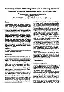
Emerging airborne networked systems require multihop transmission of data in a highly dynamic environment. An example motivation is the iNET telemetry application [1]– [4]. However, the highly dynamic environment poses unique challenges such as short transmission times between nodes due to speed and limited connectivity due to mobility [5], [6]. Therefore, a domain specific geolocation-based routing protocol, AeroRP, is proposed for multihop routing in networked systems [7]. The main focus of AeroRP is to efficiently route data packets, such as telemetry data, among airborne nodes (ANs) to a ground station (GS) as shown in Figure 1. The ANs must use themselves or relay nodes (RNs) as next hops in order for the packets to reach their destination as the AN may never be within transmission range of the GS within a reasonable amount of time. Mobile ad hoc networks (MANETs) are self-configuring wireless networks with no pre-established infrastructure. Routing packets among a network in which a specific hop-by-hop path will most likely not persist must be a major consideration by the MANET routing protocol since ANs can have relative speeds up to Mach 7 [5], [8]. These fast moving nodes create a unique challenge for routing packets when connectivity among the nodes is very intermittent and episodic. Thus, traditional MANET routing protocols are not suitable for such environments. Previous geographic-based routing protocols generally do not consider high velocity of the nodes. In this paper, we first present an overview of the AeroRP protocol and algorithm to make decisions to forward the

AN ! airborne node GS ! ground station RN ! relay node GW ! gateway

978-1-61284-254-7/11/$26.00 ©2011 IEEE

Fig. 1.

Aeronautical network architecture

packets to the next best available hop. We also present performance results of the AeroRP routing protocol and compare its performance to traditional MANET protocols. We show that certain modes of AeroRP outperform the MANET routing protocols in terms of successful packet delivery, accuracy, overhead, and delay in this highly-dynamic environment. The rest of the paper is organized as follows: Section II discusses background information specific to geographic routing protocols, some specific geographic routing protocol implementations, and routing data in high speed networks. The AeroRP routing protocol is detailed in Section III. Then, in Section IV, we present the simulation results comparing AeroRP to traditional MANET protocols in a highly dynamic network. Finally, conclusions are presented in Section V. II. BACKGROUND The various geographic routing survey papers [9]–[11] break down different geographic forwarding decisions into MFR (most forward with radius r), NFP (nearest with forward progress), and compass. MFR is the most intuitive and forwards the packet to the node that makes the most forward progress with respect to the source and destination. NFP

492

forwards the packet to the node that is closest to the source and is closer to the destination, reducing packet collisions compared to MFR by making shorter hop routing decisions. Compass forwarding chooses a node that is closest to an imaginary line drawn between the source and the destination and makes forward progress. There are many popular geographic routing protocols, including DREAM [12], LAR [13], and GPSR [14], which are reviewed in the following subsections. A. DREAM In the Distance Routing Effect Algorithm for Mobility (DREAM), the frequency at which location information is shared among the nodes is based on how far apart the nodes are and how fast the nodes are moving. The further apart a given node is from another node, the less frequent location information needs to be shared. DREAM optimizes the frequencies of its control messages based on this concept. Based on the location information that the nodes collect from their neighbors, DREAM moves the data packets with no pre-established route to nodes that it knows are towards the direction of the destination. A packet is sent among a node’s one-hop neighbors by sending to all of the neighbors that lie within a wedge that originates from the sender and opens up to the possible distance that the receiver travels in a given unit of time. The maximum velocity is used to calculate the possible distance that the destination could move. This process is repeated at each hop with an undefined recovery mechanism if there are no one-hop neighbors within the wedge. B. LAR Location-Aided Routing (LAR) uses the same concept from DREAM of the wedge and refers to it as the request zone. However, unlike DREAM, it uses this request zone to send route requests as opposed to data packets. LAR degrades to flooding if route requests to nodes within the request zone do not reach the destination. In LAR, nodes must know if they are in the request zone so they can either drop or send the route request. The LAR uses two different schemes for a node to determine if it is in the request zone. The first scheme consists of the sender sending a route request that contains the coordinates of a rectangle that contains the request zone. A node that receives this route request will discard if it is not within the rectangle and forward if it is. The second schema does not explicitly define the request zone but instead forwards the packet based on the distance the sender is from the destination. C. GPSR Greedy Perimeter Stateless Routing (GPSR) [14] forwards data packets based on a greedy heuristic. A beaconing mechanism is used to share location information with one-hop neighbors as well as piggybacking location information on actual data packets. However, packets cannot always be forwarded with this greedy approach even when other paths exist. GPSR takes another approach when greedy forwarding does not

work: perimeter routing. Well known techniques for traversing the perimeter of a planar graph are used to forward the packet until greedy forwarding can resume. D. Routing among High Speed Nodes Geographic routing in MANETs that are traveling at supersonic speeds have not been widely studied, defined by the iNET (Integrated Networked Enhanced Telemetry program) as Mach 3.5 (1200 m/s) [2]. Unpiloted aerial vehicle (UAV) geographic routing has been simulated at 25 m/s [15], much slower than Mach 3.5 (1200 m/s). A top speed of 20-50 m/s is typical among geographic routing protocols [16]–[23]. A top speed of 200 m/s has been considered while reducing the control overhead in MANETs [24]. There are a few routing protocols specifically for aeronautical environments. ARPAM [25] is a hybrid AODV [26] protocol for commercial aviation networks that utilizes the geographic locations to discover the shortest but complete end-to-end path between source and destination. Multipath Doplar routing (MUDOR) [27] takes relative velocity into consideration as well as the Doppler shift to measure the quality of a link. Anticipatory routing [28] tracks highly mobile endpoints that reach the reactive limit in which the speed of the nodes is comparable to the time it takes for the location tracking to converge upon the position of the node. Spray routing [29] involves unicasting a packet a specific depth away from the destination in which the packet is then sprayed or multicasted to a controlled width or number of levels of neighbors, for highly mobile endpoints up to 250 m/s. However, none of these approaches mention such speeds as high as Mach 3.5 in which rapidly varying connectivity is a major consideration. III. A ERO RP AeroRP makes its routing decisions with no end-to-end knowledge of a source to destination route. The routing decisions are made per-hop such that the packet is moved closer to the destination based on a speed-based heuristic that is calculated for each one-hop neighbor. The following subsections detail the calculations that are used for next hop forwarding decisions as well as the specifics of the architecture and different modes of AeroRP. A. Decision Metrics The time to intercept (TTI) is the primary metric used for routing decisions in AeroRP [7], [30]. The TTI is a heuristic metric that gives the source node an idea of how soon potential neighbors will be within transmission range of the destination. The speed component, sd , is an important part of the TTI calculation, and is the relative velocity a potential neighbor has with respect to the destination. A high and positive sd infers the neighbor is moving towards the destination at a high speed; high and negative sd infers the neighbor is moving away. In the following subsections, the sd and TTI calculations are detailed.

493

1) Speed Component: Given a neighbor ni that has geographical coordinates of xi , yi and a velocity of vxi , vyi , the velocity vector for ni is calculated as: ! vi = vxi 2 + vyi 2 (1)

the soonest and thus has the lowest TTI. Given a potential neighbor ni with coordinates xi , yi , zi and destination D with coordinates xd , yd , zd , the Euclidean distance between the two is: " (5) ∆d = (xd − xi )2 + (yd − yi )2 + (zd − zi )2

180 (2) π Destination D has geographical coordinates xd , yd . The angle between the positive x-axis of ni plane and the imaginary line drawn between ni and D is: ¯ = atan2(yd − yi , xd − xi ) × 180 Θ (3) π ¯ gives the angle The difference between the angles (Θ − Θ) between ni velocity and the imaginary line drawn between ni and D. This gives us sd :

TTI=0 is a special case that indicates to never choose this neighbor as a next hop because we do not choose nodes that are moving away from the destination and not within transmission range. A negative TTI is allowed because this is an indication of a node being within transmission range of the destination and thus should be considered as a next hop. Nodes within transmission range of the destination are chosen over nodes that are not.

The angle in degrees1 between the positive x-axis of ni plane and ni velocity vector is: Θ = atan2(vyi , vxi ) ×

¯ sd = vi cos(Θ − Θ)

(4)

Figure 2 illustrates an example in which a potential neighbor is moving towards the destination in quadrant I relative to the destination. In this example vxi is −14.15 m/s, vyi is ¯ is −111.8 ◦ , and sd is calculated −14.15 m/s, Θ is −135 ◦ , Θ as 18.4 m/s.

ni

4 135.0q

4 111.8q

135.0q  (111.8q) 23.2q

Fig. 2.

Potential neighbor moving towards destination

2) Time to Intercept: The time to intercept (TTI) is the primary metric used for routing decisions in AeroRP. A source node calculates the TTI of its neighbors to understand when it will potentially be within transmission range of the destination and make the decision to route to the neighbor that will potentially be within transmission range of the destination 1 atan2(x,y) is a two-argument convenience function that computes the angle in radians between the positive x-axis of a plane and the x, y coordinates.

The TTI is calculated as follows in which R is the transmission range of the mobile devices:  0 for sd < 0 and ∆d > R TTI = ∆d − R (6)  otherwise sd

B. Operation The AeroRP routing protocol has both a neighbour discovery and a data forwarding phase. In order to discover neighbors in beacon mode, nodes receive AeroRP hello beacons from their neighbors that contain coordinate and velocity data from that neighbor. A node maintains its neighbor table based on the hello beacons received from its neighbors. This neighbor table is used to calculate the TTI of its neighbors in order to make routing decisions. Given the wireless nature of node communication in MANETs, it is possible for a node to be promiscuous and overhear all packets, even those packets that are not intended for a given node. In beaconless promiscuous mode, AeroRP takes advantage of this behavior and adds location information to each data packet per-hop as opposed to sending periodic hello beacons with this information. All nodes within transmission range, including those nodes that are not the intended receiver, can listen to the data packet and extract the location information from the header and store this location information in its neighbor table for making routing decisions. For the case when the node receives a packet for which the node itself has the best TTI but is not within transmission range of the destination, the packet can be queued in a configurable sized queue for a configurable amount of time. The queue is checked at a configurable frequency to see if there is a neighbor with a lower TTI than the local node. When a neighbor with a lower TTI is encountered, the packets from the queue are sent at a configurable data rate. There are currently three different AeroRP modes for when the local node has the best TTI: 1) Ferry: Queue the packets indefinitely until a node with a lower TTI is found. 2) Buffer: Queue the packets in a finite sized queue with a finite timeout until a node with a lower TTI is found. 3) Drop: Drop the packet.

494

TABLE I S IMULATION VARIABLES Values Random waypoint (0 s pause) Mach 3.5 (1200 m/s) 10 150 km2 Random rectangle 100 s 1000 s wifib-11mbs 1000 bytes 8 kb/s CBR No No Friis 27.8 km UDP

• •

When receiving a data packet, a node uses its neighbor table to decide how to route the packet. If the node is not the packet’s destination, the node will clean its neighbor table of stale entries and those nodes that are predicted to be out of range. If one of the neighbors is the destination of the packet, the packet will be transmitted to the destination. Otherwise, the packet will be transmitted to a neighbor that has a better TTI. If the local node has the best TTI, it will ferry, buffer, or drop the packet depending on the mode that AeroRP is in. IV. P ERFORMANCE A NALYSIS In this section, we present the results of simulations conducted with the ns-3 simulator [31] to compare the performance of AeroRP and its various modes with the traditional MANET routing protocols AODV (ad-hoc on-demand distance vector) [26], DSDV (destination-sequenced distance vector)2 [33], and OLSR (optimized link state routing) [34], [35]. The topology setup consists of between 10 and 100 wireless ANs that are randomly distributed over the simulation area. A single stationary sink node is located in the center of the simulation area representing the ground station. AeroRP is tested in the ferrying, buffer, and drop modes that were discussed in Section III-B. In buffer mode, the packet queue size and timeout is configured to be in line with what AODV and DSDV implement. AeroRP is tested with these three modes as well as in both beacon and beaconless promiscuous mode. Other details of the simulation are shown in Table I. These parameters are chosen to identify routing performance and not to focus other layer issues [36]. 802.11b with 11 Mb/s was the most common and reliable wireless link layer protocol in ns-3 at the time of the AeroRP implementation. We look at four different metrics to measure the performance of the different routing algorithms: • Packet delivery ratio (PDR): the number of packets received divided by the number of packets sent at the application layer. Note that not necessarily all packets sent at the application layer will be sent at the MAC layer. This can happen if there is no route for the packet. 2 AODV and OLSR is part of the standard ns-3, DSDV has been developed by the KU ResiliNets group and has been merged into ns-3.10 [32].

Accuracy: the number of packets received divided by the number of packets sent at the MAC layer. This allows us to measure how accurate a route is for a given routing protocol based on whether or not the route that was chosen for the packet results in a successful reception at the destination. This is a good metric to gauge the quality of a route in a highly dynamic topology in which the validity of a route can rapidly change. Overhead: the excess Bytes used to move the actual packet payload from source to destination. Delay: the difference in time between when the originator of a data packet transmits the packet at the MAC layer and the time that the MAC layer of the final destination receives the data packet.

Figure 3 shows the average PDR as the number of nodes are increased. The node density of the network affects all of the routing protocols with AeroRP ferrying packets in beaconless promiscuous mode performing the best. The PDR for all AeroRP modes increases as the number of nodes increase with the exception of a slight performance degradation as the number of nodes approaches 90 and higher. The PDR for both DSDV and AODV immediately degrades as the number of nodes increases. This is most likely due to the increase in overhead observed as the number of nodes increases. The performance of OLSR starts to degrade around 50 nodes. This suggests that as the number of nodes increase, AeroRP is able to make more intelligent decisions on how to move the data packets towards the destination whereas the non-AeroRP routing protocols are relying on non-geographic based links to move the packet to the destination. 0.7

average packet delivery ratio

Variable Mobility model Velocity Simulation runs Simulation area Initial position allocator Warmup time Application sending time Link layer Packet size Sending rate RTS/CTS? Packet fragmentation? Propagation loss model Transmission range Transport protocol

•

0.6

0.5

0.4

0.3

AeroRP - Drop:Beacon AeroRP - Drop:Beaconless AeroRP - Ferry:Beacon AeroRP - Ferry:Beaconless AeroRP - Buffer:Beacon AeroRP - Buffer:Beaconless OLSR DSDV AODV

0.2

0.1

0.0 10

20

30

40

50

60

70

80

90

100

number of nodes Fig. 3.

Effect of node density on PDR

Figure 4 shows how accurate the various routing protocols are as the number of nodes are increased. OLSR, DSDV, and AODV yield an accuracy of less than 62%. All of the various modes of AeroRP have an accuracy of 50% or higher at all node densities. The accuracy of ferrying and buffering packets with AeroRP stays constant at almost 100% as the number of nodes increases. This illustrates AeroRP’s ability to accurately deliver packets, largely facilitated by predicting

495

1.0 0.9

average accuracy

0.8 0.7 0.6 AeroRP - Drop:Beacon AeroRP - Drop:Beaconless AeroRP - Ferry:Beacon AeroRP - Ferry:Beaconless AeroRP - Buffer:Beacon AeroRP - Buffer:Beaconless OLSR DSDV AODV

0.5 0.4 0.3 0.2 0.1 0.0 10

20

30

40

50

60

70

80

90

100

number of nodes Fig. 4.

Effect of node density on accuracy

As illustrated in Figure 5, the average overhead of the network increases with the node density. However, the proactive discovery and maintenance of routes in AODV results in exponentially increasing overhead as the number of nodes increase from 30 to 50 nodes. The overhead of AODV would probably continue to exponentially increase and monopolize the bandwidth if it did not hit the network saturation point. The overhead of DSDV increases linearly from 18 kb/s at 10

nodes to 1.5 Mb/s at 100 nodes. The overhead of OLSR and the AeroRP routing protocols also increase linearly, but not as drastically as DSDV, from around 15 kb/s at 10 nodes to around 100 kb/s at 100 nodes. OLSR is similar to AeroRP in that it proactively beacons control messages to it’s one-hop neighbors. Note that AeroRP in beaconless promiscuous mode with no ferrying has the lowest overhead. This makes sense because the beaconless promiscuous mode removes the need for separate control packets, thus cutting down on overhead. Also, this mode of AeroRP transmits less packets because it drops them immediately if there is no route, which also cuts down on overhead. 1E+04

average overhead [kb/s]

whether fast moving neighbors are in or out of transmission range by using the last known distance between the source and neighbor as well as the neighbor’s velocity. Of the AeroRP modes, the beaconless promiscuous mode is more accurate than the beacon modes for two reasons. First, the surrounding nodes overhear data packets and thus trajectory data every single time a packet is transmitted. This results in sharing trajectory information more often than sending out periodic hello beacons. Second, putting the control data in the actual data packets makes the communication more symmetric than sending separate control packets. A control packet that is 44 B may be transmitted successfully to a neighbor. However, this does not necessarily mean that a 1000 B payload plus the control overhead can be successfully transmitted to that same neighbor, especially if that neighbor is on the edge of the transmission range. For AeroRP, the accuracy increases with the node density with the exception of AeroRP running in beaconless promiscuous mode but with no ferrying or buffering of packets. This decrease in accuracy can be attributed to the nodes having to rely on data transmissions to communicate their trajectories to nearby nodes. The buffering and ferrying allows data to be delivered at different times in the simulation whereas AeroRP that is not ferrying or buffering packets is not sharing this information as often. This does not occur when AeroRP is in beacon mode but not ferrying or buffering packets because it still regularly shares its trajectory information with its neighbors in the form of periodic hello beacons. OLSR yields higher accuracy as the number of nodes increases but still not as high as the AeroRP modes.

1E+03

1E+02

AeroRP - Drop:Beacon AeroRP - Drop:Beaconless AeroRP - Ferry:Beacon AeroRP - Ferry:Beaconless AeroRP - Buffer:Beacon AeroRP - Buffer:Beaconless OLSR DSDV AODV

1E+01

1E+00 10

20

30

40

50

60

70

80

90

100

number of nodes

Fig. 5.

Effect of node density on overhead

The effect that node density has on the delay of data packet transmissions is shown in Figure 6. AeroRP modes that ferry or buffer packets have the highest delay because the packet will be held as long as required for delivery or until the packet expires in the queue in buffer mode. The delay could be as long as required for a given scenario assuming the protocol and end point can tolerate such delay (e.g. nonreal time communication). Although the delay is higher, these modes usually deliver more packets than the other protocols as previously shown in Figure 3. The two AeroRP modes that buffer packets have delay in the middle compared to the other routing protocols because they will only hold packets for a finite amount of time. The two AeroRP modes that do not do packet ferrying or buffering have the lowest delay because they drop the packet immediately if there is no route. It is interesting to note that the ferrying and buffering modes of AeroRP actually decrease in delay as the node density increases while the other AeroRP modes, AODV, DSDV, and OLSR actually increase in delay as the node density increases. Perhaps as the node density increases, the buffering and ferrying modes are able to get their buffered and ferried packets to their destinations more quickly while the increase in nodes results in more hops and thus longer delay to the destination. It is suspected that calculating just the average delay for data packets that were not ferried or buffered for the AeroRP modes that do this would result in the same increasing trend of delay as the number of nodes increases.

496

1E+05

average delay [ms]

1E+04

1E+03

1E+02 AeroRP - Drop:Beacon AeroRP - Drop:Beaconless AeroRP - Ferry:Beacon AeroRP - Ferry:Beaconless AeroRP - Buffer:Beacon AeroRP - Buffer:Beaconless OLSR DSDV AODV

1E+01

1E+00 10

20

30

40

50

60

70

80

90

100

number of nodes

Fig. 6.

Effect of node density on delay

V. C ONCLUSIONS Highly-dynamic airborne networks require domain-specific protocols for communication to cope with the challenges faced in highly-dynamic environments. In this paper, we detail AeroRP, a geographic-based routing protocol designed specifically for high-speed environments. Furthermore, we present the results of simulating AeroRP and other legacy MANET routing protocols in high-velocity scenarios. The combination of some kind of packet buffering, whether it is indefinite or finite, coupled with beaconless promiscuous mode generally yields the best PDR, accuracy, and overhead. The AeroRP buffering modes offer a tradeoff between the higher packet delivery but higher delay of the ferrying modes. ACKNOWLEDGMENTS The authors would like to thank the Test Resource Management Center (TRMC) and the Test and Evaluation/Science and Technology (T&E/S&T) Program for their support. This work was funded in part by the T&E/S&T Program through the Army PEO STRI Contracting Office, contract number W900KK-09-C-0019 for AeroNP and AeroTP: Aeronautical Network and Transport Protocols for iNET (ANTP). This work was also funded in part by the International Foundation for Telemetering (IFT). We would like to acknowledge ResiliNets group members Justin P. Rohrer for useful discussions. We would also like to thank Kip Temple and the membership of the iNET working group for discussions that led to this work. R EFERENCES [1] [2] [3] [4] [5]

iNET Working Group, “http://www.inetprogram.org.” “iNET Needs Discernment Report, version 1.0.” CTEIP, May 2004. “iNET Technology Shortfalls Report, version 1.0.” CTEIP, July 2004. “iNET System Architecuture, version 2007.1.” CTEIP, July 2007. J. P. Rohrer, A. Jabbar, E. K. C¸etinkaya, and J. P. Sterbenz, “Airborne Telemetry Networks: Challenges and Solutions in the ANTP Suite,” in IEEE MILCOM, (San Jose, CA, USA), pp. 772–777, November 2010. [6] J. P. Rohrer, A. Jabbar, E. K. C¸etinkaya, E. Perrins, and J. P. Sterbenz, “Highly-dynamic cross-layered aeronautical network architecture,” IEEE T. on Aero. and Elec. Sys. (TAES), vol. 47, October 2011. to appear. [7] A. Jabbar and J. P. Sterbenz, “AeroRP: A Geolocation Assisted Aeronautical Routing Protocol for Highly Dynamic Telemetry Environments,” in International Telemetering Conference, Oct. 2009.

[8] J. P. Rohrer, A. Jabbar, E. Perrins, and J. P. Sterbenz, “Cross-Layer Architectural Framework for Highly-Mobile Multihop Airborne Telemetry Networks,” in IEEE MILCOM, pp. 1–9, Nov. 2008. [9] M. Mauve, A. Widmer, and H. Hartenstein, “A Survey on PositionBased Routing in Mobile Ad Hoc Networks,” IEEE Network, vol. 15, no. 6, pp. 30–39, 2001. [10] C. Lemmon, S. M. Lui, and I. Lee, “Geographic Forwarding and Routing for Ad-hoc Wireless Network: A Survey,” in IEEE NCM, pp. 188–195, 2009. [11] M. de la Fuente and H. Ladiod, “A Performance Comparison of PositionBased Routing Approaches for Mobile Ad Hoc Networks,” in IEEE VTC, pp. 1–5, Sept. 2007. [12] S. Basagni, I. Chlamtac, V. R. Syrotiuk, and B. A. Woodward, “A Distance Routing Effect Algorithm for Mobility (DREAM),” in ACM MobiCom, pp. 76–84, 1998. [13] Y.-B. Ko and N. H. Vaidya, “Location-aided Routing (LAR) in Mobile Ad Hoc Networks,” in ACM MobiCom, pp. 66–75, 1998. [14] B. Karp and H. T. Kung, “GPSR: Greedy Perimeter Stateless Routing for Wireless Networks,” in ACM MobiCom, pp. 243–254, 2000. [15] R. L. Lidowski, B. E. Mullins, and R. O. Baldwin, “A Novel Communications Protocol using Geographic Routing for Swarming UAVs Performing a Search Mission,” in IEEE PERCOM, pp. 1–7, 2009. [16] E. Kuiper and S. Nadjm-Tehrani, “Geographical Routing in Intermittently Connected Ad Hoc Networks,” in IEEE AINI, pp. 1690–1695, March 2008. [17] B. Zhou, Y.-Z. Lee, and M. Gerla, “Direction Assisted Geographic Routing for Mobile Ad Hoc Networks,” in IEEE MILCOM, pp. 1–7, Nov. 2008. [18] Z. Jin, N. Yan, and L. Bing, “Reliable On-Demand Geographic Routing Protocol Resolving Network Disconnection for VANET,” in IEEE WiCOM, pp. 1–4, Sept. 2009. [19] S. Jung et al., “A Geographic Routing Protocol Utilizing Link Lifetime and Power Control for Mobile Ad Hoc Networks,” in ACM FOWANC, pp. 25–32, 2008. [20] Q. J. Chen et al., “Adaptive Position Update in Geographic Routing,” in IEEE ICC, vol. 9, pp. 4046–4051, June 2006. [21] J. Na and C. kwon Kim, “GLR: A novel geographic routing scheme for large wireless ad hoc networks,” Computer Networks, vol. 50, no. 17, pp. 3434–3448, 2006. [22] J. Li and S. Shatz, “Toward Using Node Mobility to Enhance Greedyforwarding in Geographic Routing for Mobile Ad Hoc Networks,” in Proc. of MODUS, pp. 1–8, April 2008. [23] W. Su, S. Lee, and M. Gerla, “Mobility prediction and routing in ad hoc wireless networks,” Int. J. Netw. Man., vol. 11, no. 1, pp. 3–30, 2001. [24] E. Sakhaee et al., “A Novel Scheme to Reduce Control Overhead and Increase Link Duration in Highly Mobile Ad Hoc Networks,” in IEEE WCNC, pp. 3972–3977, 2007. [25] M. Iordanakis et al., “Ad-hoc Routing Protocol for Aeronautical Mobile Ad-Hoc Networks,” in Proc. of CSNDSP, pp. 543–547, 2006. [26] C. Perkins, E. Belding-Royer, and S. Das, “Ad Hoc On-Demand Distance Vector (AODV) Routing.” RFC 3561 (Experimental), July 2003. [27] N. K. E. Sakhaee, A. Jamalipour, “Aeronautical Ad Hoc Networks,” in IEEE WCNC, vol. 1, pp. 246–251, April 2006. [28] F. Tchakountio and R. Ramanathan, “Anticipatory Routing for Highly Mobile Endpoints,” in Proc. of IEEE WMCSA, pp. 94–101, 2004. [29] F. Tchakountio and R. Ramanathan, “Tracking Highly Mobile Endpoints,” in ACM WoWMoM, pp. 83–94, 2001. [30] K. Peters, E. K. C ¸ etinkaya, A. Jabbar, and J. P. G. Sterbenz, “Analysis of a Geolocation-Assisted Routing Protocol for Airborne Telemetry Networks,” in International Telemetering Conference, Oct. 2010. [31] “The ns-3 Network Simulator.” http://www.nsnam.org, July 2009. [32] J. P. Rohrer, E. K. C¸etinkaya, A. Jabbar, D. Broyles, K. Peters, H. Narra, Y. Cheng, K. S. Pathapati, and S. Simpson, “ResiliNets models and tools for ns-3 network simulator.” http://wiki.ittc.ku.edu/resilinets/Models and Tools for ns-3 Network Simulator, December 2010. [33] C. E. Perkins and P. Bhagwat, “Highly Dynamic Destination-Sequenced Distance-Vector Routing (DSDV) for Mobile Computers,” in ACM SIGCOMM, pp. 234–244, 1994. [34] P. Jacquet et al., “Optimized Link State Routing Protocol for Ad Hoc Networks,” in Proc of IEEE INMIC, pp. 62–68, Aug. 2002. [35] T. Clausen and P. Jacquet, “Optimized Link State Routing Protocol (OLSR).” RFC 3626 (Experimental), Oct. 2003. [36] K. Peters, J. P. Rohrer, and J. P. Sterbenz, “Validation and Benchmarking of ns-3 Wireless Models,” 2010. submitted.

497