Geographical Routing Using Partial Information for ... - Semantic Scholar

Geographical Routing Using Partial Information for Wireless Ad Hoc Networks Rahul Jain, Anuj Puri and Raja Sengupta Department of EECS, University of California, Berkeley (rjain,anuj,sengupta)@EECS.Berkeley.EDU December 20, 1999

Abstract In this paper, we present an algorithm for routing in wireless ad hoc networks using information about geographical location of the nodes. We assume each node knows its geographical position and the position of the node to which it wants to send a packet. Initially, the nodes only know their neighbors but over time they discover other nodes in the network. The routing table at a node S is a list h(pi ; Si )i where pi is a geographical position and Si is a neighbor of node S . When node S receives a packet for a node D at position pos(D), it finds the pi in its routing table which is closest to pos(D) and forwards the packet to the neighbor Si . We prove the correctness of the algorithm and show that our algorithm naturally aggregates the nodes so that the routing table sizes are of size O(Ln log(n)), where Ln is the mean route discovery path length, and n is the number of nodes. We also present methods for taking positional errors, node failures and mobility into account. We justify the results through simulation.

1 Introduction A wireless ad hoc network consists of a collection of mobile nodes sharing a wireless channel without any centralized control or established communication backbone. Each node communicates with other nodes within its transmission range. To send a packet to a destination, a node forwards the packet to its neighbor which in turn forwards it to its neighbor and so on, until the packet reaches the destination. The topology of the ad hoc network depends on the location of the mobile nodes and maybe changing with time. Some of the typical applications of ad hoc networks are in scenarios where setting up a communication infrastructure is difficult (because of mobility) or very expensive (because of terrain). Wireless ad hoc networks can be used in battlefield situations where a communication infrastructure is difficult to build and maintain. Ad hoc networks are also of interest for traffic control in automated vehicle navigation systems [15]. Other commercial applications include building a wireless access infrastructure such as the ones being built by Metricom and Rooftop. Researchers are also exploring the use of ad hoc networks in building networks out of a large number of tiny sensors spread over a geographic area. In this paper, we will be interested in the routing problem in ad hoc networks. Basic routing algorithms such as link or distance-vector routing require every node to learn about every other node in the network. We refer to this as routing based on full information. This is in contrast to routing under partial information. In  This work was supported by the ONR grant N0014-99-1-0695. It has been published as the technical Memorandum no.

UCB/ERL M99/69

1

this kind of routing, a node routes based on information about a subset of the nodes in the network. Routing in the Internet provides one example. Routing in the Internet relies on the address hierarchy that mimics the network topology to work correctly. Thus, routing table sizes are manageable and changes in every link of the network do not have to be propagated throughout the network. In flat distance-vector or link-state routing, these savings are not obtained. Since ad-hoc networks change topology frequently, routing under partial information is of interest for ad-hoc networks. The Zone Routing Protocol is one well known example of an algorithm based on partial information. A node is expected to know the topology in its own zone accurately, and that in other zones only approximately. It is hoped that this will reduce the inter-node communication required to track a changing network topology. Of course, the reduction in the information used for routing may impose other costs. For example, the routes may not be shortest paths. This paper presents a new type of distributed, adaptive and asynchronous routing algorithm for ad-hoc networks. It routes based on partial information. It does not rely on any address hierarchy but instead relies on information about node positions, and hence, is called the geographical routing algorithm (GRA). We assume each node knows its own position, and can acquire the position of the packet destination by some means. Initially, each node only knows about its neighbors. The routing table at a node S is a list h(pi; si)i where pi is a position and si is a neighbor of S . When node S receives a packet for destination D, it finds the pi which is closest to pos(D), the position of D, and forwards the packet to neighbor si . The neighbor then repeats the same procedure. In this way, the packet makes its way to destination D. But sometimes when routing a packet, node S may discover that it is closer to the destination than any other position pi . In this case we say the packet is “stuck” at S . This causes a route discovery protocol to be started. The route discovery protocol finds a path from S to D and updates the routing table of the node ki on the path by placing the entry (pos(D); ki+1) in its routing table where ki+1 is the node which follows ki on the path. In this way new routing entries get added to the routing tables. After the route discovery protocol is completed, the stuck packet can be routed from S to D. We show that the routing table sizes of our nodes remain fairly small - essentially logrithmic in the number of nodes in the network. Most network routing algorithms do not use position information. However, the results in this paper show that the use of such information in ad-hoc network routing could yield large reductions in routing table size and protocol overhead. We show that the GRA has the same basic properties as most other routing algorithms even though it works with partial information. Given an unknown network, nodes will exchange information and converge to a set of routing tables. We also show that once the routing tables have converged, like other routing algorithms, all routes are acyclic. On the negative side, it should be noted that the GRA does not attempt at shortest path routing. It just uses some acyclic route. We have confined our discussion to static networks so far. In a dynamic network, links will break and form, nodes will join and leave. The number of protocol packets triggered by each such change should be of the same order of magnitude as characterized in Section 6.4. As we develop mobility models for application environments of interest to us we hope to find out whether these overheads are indeed small enough. In Section 2, we discuss the GRA in relation to other routing algorithms in the literature. Section 3 presents the system model and problem statement. Section 4 describes the geographical routing algorithm. Sections 5 and 6 discuss issues related to position information inaccuracy and inconsistency, and mobility. Section 7 presents simulation results. Section 8 concludes the paper.

2 Literature Review In the literature, a number of proposals have been made to solve the problem of routing in wireless ad hoc networks [8, 9, 10, 12, 13, 6, 14]. Most of the approaches are based on the source routing and distance-vector 2

routing approaches. The destination sequenced distance vector (DSDV) [11] routing protocol is based on the classical distance vector algorithm which uses the Distributed Bellman-Ford algorithm (DBF) [7]. The algorithm has modifications to avoid the looping problem present in the basic DBF. Formation of cycles are avoided by tagging each routing table entry with a sequence number. Dynamic source routing (DSR) [5] on the other hand is based on source routing, where the source specifies the complete path to the destination in the packet header and each node forwards the packet to the node specified as the next hop in the packet header. Each source maintains a route cache, where it looks for a path to the destination. If such a path is not found then the source initiates a route discovery protocol to discover the route. Most of the approaches in the literature are variants of the two above approaches with some attempting to combine the best of both. For example, in zone routing protocol (ZRP) [4], each node has a “routing zone” which includes the nodes within some specified distance. Each node knows the topology within its routing zone by using DSDV protocol. For out-of-zone destinations, DSR is used. Other existing proposals are based on finding a backbone for the network (MCDS) [1] or attempt to minimize delay (STARA) [2].

3 System Model and Problem Statement Suppose there are n nodes in a region that want to communicate with each other. Each node using a wireless link can communicate with only a small subset of the nodes that are its neighbors. When a node S wants to transmit a packet to a destination D, it transmits to a neighbor, which in turn transmits to its neighbor, and so on, until the packet reaches destination D. In a wireless network, each node has a trans-receiver that it uses to communicate. The set of nodes with which a node can directly communicate is not fixed but depends on the power used by its radio transmitter. When the power of the radio transmitter is increased, a node can directly communicate with a larger set of nodes (i.e., it has a larger number of neighbors). In this paper, we will assume that the nodes have fixed the optimal power for their trans-receivers and the neighbors with which a node communicates is hence fixed. Then, we can think of the wireless network as a graph G = (N; E ) where the nodes are N = f1; : : : ; ng and there is an edge (i; j ) 2 E if i is a neighbor of j in the wireless network. We assume that i is a neighbor of j if and only if j is a neighbor of i in the wireless network. Then, we can think of the links as being symmetric and the resulting graph as undirected. Furthermore, we assume that the power levels of the trans-receivers are chosen so that the resulting graph is connected. We will also assume that there exists a medium access schedule such that each node can transmit at a certain bit rate without interference. In this paper, we solve the problem of routing using position information. When a node receives a packet for destination D, it must make a routing decision: which neighbor should the packet be forwarded to? We assume the nodes f1; : : : ; ng haves names or IP addresses fS1 ; : : : ; Sn g and are located at positions fpos(S1); : : : ; pos(Sn)g. Each node knows its neighbors and its own position. When a node Si wants to send a packet to node D, it finds out the position using some position look-up service and addresses the packet to position pos(D). The geographical routing algorithm uses only the position information in making its routing decisions. How the lookup service works, and how a node finds its own position and the position of the destination is not the subject of this paper though we discuss it briefly below. To decide to which neighbor a packet should be forwarded to, a node consults its routing table. A routing table of node S is a list f(pi; Si)g (containing in general, fewer entries than the total number of nodes in the network) where pi is a geographical position and Si is a neighbor of S . When node S receives a packet for destination position D, it finds the position pi which is closest to D and forwards the packet to neighbor Si . We assume initially the nodes only know their neighbors and have no knowledge of the topology. The subject of this paper is how the nodes construct their routing tables in an online manner, why the routing algorithm works correctly and what its performance is.

3

3.1 Finding position information We assume that each node can find its own position and the position of the destination node. Although how this is done is not the subject of this paper, we sketch out some technologies which make it feasible. Using the global positioning system (GPS), it is now possible for any node to find its geographical position with a small error. GPS receivers are cheaply available and more precise devices using differential GPS are also available. In applications where the IP address is known but the geographical address is not, a separate translation protocol must be used to find the geographical position from the IP address. This could for example be done using a two way paging network where the IP address is broadcast to all nodes and the node with that specific IP address replies back with its geographical position. Again the details of how this is done are beyond the scope of this paper.

4 The Geographical Routing Algorithm In this section, we describe the geographical routing algorithm which we refer to as the GRA in short. The basic idea behind the algorithm is to use the geographical position of the destination in making routing decisions. Each node only knows about a small number of nodes in the network. It knows more about nodes that are nearer to it than it does about nodes which are further away. When a node has a packet for a destination, it chooses from the nodes it knows about the one which is closest to the destination, and sends the packet on its way to that node. Along the path, a node may know of an even closer node to the destination. The packet then gets redirected to that node. On its way to that node, it may get redirected again, and so on until it reaches the destination. For example, suppose a packet is to be sent from from New York city to UC Berkeley, CA. Suppose the New York city node “knows” the route to a node in San Francisco, CA. It then routes the packet according to that node. On the way suppose, there is a node that “knows” a better route to Berkeley, CA. It then routes the packet onto the better route. Now, suppose the packet reaches near Bay Area, and a node “knows” an even better route to UC Berkeley. It, then, routes the packet onto this route, and the packet thus reaches the node in UC Berkeley. Thus, the algorithm has an in-built capability of finding better and better routes to the destination as the packet nears the destination, even though the source node “knows” the network topology around the destination very “coarsely”. We now describe the routing algorithm in detail, and prove its correctness by showing that routing tables are cycle-free and that packets reach their destination. We also quantify the performance of the algorithm in terms of the average routing table lengths.

4.1 The Algorithm Suppose G = (N; L) is the graph corresponding to our wireless network. The algorithm begins with each node initially knowing only about its neighbors. The routing table at a node S is a list f(pi; Si)g where pi is a geographical position of some node and Si is a neighbor of S . When destination D is closest to position pi in the routing table, node S forwards the packet to neighbor Si . Each node thus forwards the packet in the same way till the packet reaches the destination. But sometimes when routing a packet, node S may discover that it is closer to the destination than any other position pi . In this case we say the packet is “stuck” at S . This causes the “route discovery protocol” to be started. The route discovery protocol finds a path from S to D (say Path(S; D) = k0 k1 : : :kl ) and updates the routing table of the node ki on the path by placing the entry (pos(D); ki+1) in its routing table. So now each node on the path knows how to get to D. It is in this way that new routing entries get added to

4

the routing tables. After the route discovery protocol is completed, the stuck packet can be routed from S to D. We next present our routing algorithm in more detail. We introduce the notion of Voronoi views. This is a geometric way of viewing the routing operation. Each entry (pi ; Si) in the routing table is associated with a region in IR2 so that if the destination of a packet falls in the region, the packet gets routing according to the entry (pi; Si). 4.1.1 Voronoi Cells Let CSt = fS1; S2; ::; Skg be the set of nodes whose geographic locations are known to node S at time t (we assume S 2 CSt ). We refer to these nodes as centers at node S . We use the positions of the centers to partition IR2 into cells so that all packets for positions which fall within a cell are routed similarly. A cell around the center Si consists of all points that are closer to Si then any other Sj . We call this the Voronoi cell with center Si . We then define the Voronoi view of node S as consisting of the Voronoi cells with centers Cst. Formally, Definition 1 (Voronoi cell) Let fS1 ; S2; ::; Skg be any set of points in IR2 . A Voronoi cell with center Si is defined as

VS (Si) = fz 2 IR2 : jz ? pos(Si)j = 1min jz ? pos(Sj )j; Sj 2 CSt g j k Definition 2 (Voronoi view) The Voronoi view at node S at time t is

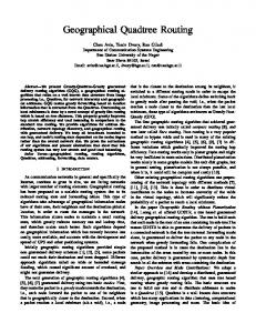
VSt = fVSt(Si) : Si 2 CSt g Example 1 (Voronoi view) The example below explains the concept of the Voronoi view. In figure 1, node S has nodes A, B , C , D in its routing table as centers but not E . Thus, the Voronoi view of S is the tessellation of the network region based on these nodes. Node E does not affect the Voronoi view of S . But if E is destination for some packet at S , then S forwards the packet to the neighbor node D, which happens to be the closest center to E in S ’s Voronoi view.

0 1 1 0 0 1

1 0 0 1

A

B

S

1 0 0 1 1 0 0 1 E

C

1 0 1 0

1 0 1 0

D

Figure 1: Example of a Voronoi view Thus, in making a routing decision for a packet going to destination D, node S looks at its routing entries f(pi; Si)g and finds the position pj which is closest to D. It then routes the packet to the neighbor of node S forming a Voronoi view based on the centers whose positions are fp1; : : : ; pkg. It then finds the cell in its Voronoi view in which the destination D lies (say pj ), and it then routes the packet to neighbor Sj , as if the packet were meant for the node at position pj . 5

4.1.2 Routing Table Structure The routing table at a node S is structured as shown in figure 2. The first column is the names of nodes that S knows about. We refer to the set of nodes in the first column as the centers at node S . The second column is the positions of the nodes in the first column. We denote this by pos(S ): The third column is a column of neighboring node names. Thus if S 0 is a node in the first column (see 4-th row of figure 2) and N 0 the node in the neighbor column for S 0 , then packets directed to VS (S 0) should be forwarded to N 0 . Sometimes, we will use the notation NextS (S 0) for N 0, where NextS (S 0) is the neighbor of S to which packets for a node in VS (S 0) should be forwarded by S . The time-stamp is the time at which the destination node replied to the route discovery message. If the network is mobile, the time-stamp could be used to decide when to obsolete the routing table entry as well. Some special features of the routing tables are as follows: Since each node is assumed to know its own position, each node has an entry for itself in its own routing table. The first row of figure 2 reflects this. The corresponding neighbor is trivially set to itself. Also, the first column of the routing table should contain all the neighbors of S . The corresponding entry in the neighbor column would be the neighbor itself. node

node position

neighbor node

S0

.

pos(S 0)

.

N0

.

.

.

S N

pos(S ) pos(N )

S N .

time stamp TS TN . TS 0 .

Figure 2: Routing table structure Each routing table entry at S is a 4-tuple (Si ; pos(Si); NextS (Si ); TSi ). When some of the fields of a routing entry are not of interest, we indicate them with a “-”, for example (?; pos(Si); NextS (Si ); ?). Sometimes, when there is no confusion, we also write this as (pos(Si ); NextS (Si )). 4.1.3 Packet Format The packet header has the information shown in figure 3 to aid routing. The source and destination unique names are specified in the packet. The destination position is also specified in the packet. The destination name and position are used for packet forwarding and route discovery. The source time-stamp, source name and source position are included in figure 3 because these may be required in an implememtation of the GRA. destination-name

destination-position

source-time-stamp

source-name

source-position

DATA

Figure 3: Packet format

4.2 Packet Forwarding Figure 4 describes the packet forwarding algorithm at each node. Suppose a node S receives a packet for destination D. Let C S denote the set of names of all the nodes that S knows about, i.e., C S is the set of names in the first column of figure 2. We use dist(S; D) to denote the distance between the nodes S and D, i.e., dist(S; D) = kpos(S ) ? pos(D)k; and id to denote the complete order on node names. The packet forwarding decision is quite simple: At any time, a node knows about only a small subset of the nodes in the network. Initially, this set consists of only the node itself and its immediate neighbors.

6

Node S receives packet for destination D at time t: Let pos(D) 2 VSt (Si ) for some Si

2 CSt

if (S == D) // packet reached its destination else if (Si 6= S ) next node = NextS (Si ); else //packet is stuck Initiate route discovery(S ,D); next node = NextS (D); Figure 4: Packet forwarding algorithm Later, the nodes that are discovered through the route discovery process are added to its routing table. When a node S receives a packet for destination position D, it finds the entry (Si; pos(Si); NextS (Si)) such that Si is closer to D then any other Sj . It then routes the packet to NextS (Si). It may turn out that node S is itself closest to D then any other Sj 2 C S . In that case, we say that packet is stuck and it cannot be forwarded to any of the neighbors according to its current routing table. If the packet is stuck, then node S initiates a route discovery to the destination node D. The route discovery procedure route discovery(S ,D) finds an acyclic path Path(S; D) = hk0; k1; : : : ; kli from S to D, and it updates the routing table of node ki with an entry (D; pD; ki+1). It is however possible that a packet destination D is equally close to two nodes Si and Sj (i.e., kpos(D) ? pos(Si)k = kpos(D) ? pos(Sj )k), and the node lies on the cell boundary. In that case, we assume there is a total order among names, and use that to resolve the tie (i.e., if Si id Sj , the packet is routed to NextS (Si ), otherwise it is routed to NextS (Sj )). Example 2 illustrates the GRA routing. Example 3 shows that the use of an order on node-names is important for acyclic routing. (2,2) B (1.5,1.5) A (3,1) C (2.5,0) D

(4,0) E

Figure 5: An example network Example 2 We illustrate our algorithm on an example network. Consider the network of Figure 5. It consists of nodes fA; B; C; D; E g which are located at positions (1:5; 1:5); (2; 2); (3; 1); (2:5; 0) and (4; 0) respectively. The links between the nodes are symmetric and given by f(A; B ); (B; C ); (C; D); (C; E )g. Initially, each node only “knows” about itself and its neighbors. The initial routing tables at the nodes are shown in Figure 6.

7

Node Routing table of A Routing table of B: Routing table of C: Routing table of D: Routing table of E:

Routing Table

f(A; (1:5; 1:5); ?); (B; (2; 2); B)g f(B; (2; 2); ?); (A; (1:5; 1:5); A); (C; (3; 1); C)g f(C; (3; 1); ?); (B; (2; 2); B); (D; (2:5; 0); D); (E; (4; 0); E)g f(D; (2:5; 0); ?); (C; (3; 1); C )g f(E; (4; 0); ?); (C; (3; 1); C )g Figure 6: Initial Routing Tables

Suppose node A gets a packet for destination C located at pos(C ) = (3; 1). Node A then looks into its routing table and finds that pos(B ) is closer to pos(C ) then pos(A). So it forwards the packet to node B . Similarly, node B looks at its routing table and finds that pos(C ) is closer to pos(C ) than either pos(A) or pos(B). So it forwards the packet to node C which is the destination. Next, suppose A gets a packet for destination D located at pos(D) = (2:5; 0). Node A looks into its routing table and finds that pos(A) is closer to pos(D) then pos(B ). So the packet becomes stuck at node A. This triggers a route discovery. The route discovery process finds the path hA; B; C; Di to the destination D. In the process it also updates the routing tables of nodes A; B and C . The new updated routing tables are shown in Figure 7. A forwards the packet for D to B which forwards it to C and C forwards it to D. Node Routing table of A: Routing table of B: Routing table of C: Routing table of D: Routing table of E:

Routing Table

f(A; (1:5; 1:5); ?); (B; (2; 2); B); (D; (2:5; 0); B)g f(B; (2; 2); ?); (A; (1:5; 1:5); A); (C; (3; 1); C ); (D; (2:5; 0); C )g f(C; (3; 1); ?); (B; (2; 2); B); (D; (2:5; 0); D); (E; (4; 0); E)g f(D; (2:5; 0); ?); (C; (3; 1); C )g f(E; (4; 0); ?); (C; (3; 1); C )g Figure 7: Updated Routing Tables

Next suppose A gets a packet for destination E located at pos(E ) = (4; 0). A looking into its routing table finds that pos(D) is closer to pos(E ) then either pos(A) or pos(B ). So it forwards the packet to node B based on the entry (D; (2:5; 0); B; ?) in its routing table. Similarly B finds that pos(E ) is closer to pos(D) then either pos(B ), pos(A) or pos(C ). So it forwards the packet to C based on the entry (D; (2:5; 0); C; ?) in its routing table. Node C finds that pos(E ) is closer to pos(E ) than pos(D) or pos(C ), so it forwards the packet to E based on the entry (E; (4; 0); E; ?). Thus, A was able to route a packet to E even though it did not have E in its routing table. Our simulations indicate that in large networks this is frequently the case. Example 3 Consider the network shown in figure 8. The routing tables at each node are as shown in the figure. For convenience we have left out the node positions from the figure. Thus T 2 : (b; 1)(a; a) is the routing table at node d: (b; 1) means that if the surrogate destination is b then the packet will be forwarded to 1. Nevertheless, the understanding is that a node knows the position of each node in its routing table. Both nodes 1 and 2 have a and b in their routing tables. Node 1 sends packets to a through 2: Node 2 sends packets to node b through 1. Now suppose 1 originates a packet for d: Since it knows both a and b which are equidistant from d; suppose it randomly selects a and forwards the packet to 2: Likewise 2 is faced with the same choice. If 2 randomly chooses b then the packet cycles. To prevent such cycles we disallow random choices between equidistant nodes. Instead we require that be resolved by the lexicographic order on node names. Thus if a id b both 1 and 2 would choose a:

8

T2: (b,1) (a,a) 2

Ta: (2,2)(d,d) a d Td: (a,a)(b,b) b

1

Tb: (1,1)(d,d)

T1: (a,2) (b,b)

Figure 8: Forwarding without the Name Order

4.3 Route Discovery Suppose node S gets a packet for destination D. The packet gets stuck at node S if the destination lies closer to S than any other cell center at S . This triggers the route discovery mechanism. which finds an acyclic path Path(S; D) from S to D. The only requirement for the route discovery mechanism is that it return an acyclic path to the destination, and that it update the routing tables on that path in an appropriate manner. Suppose the acyclic path found is Path(S; D) = hk0; k1; : : : ; kli. We then require that an entry (D; pos(D); ki+1) be added to the routing table of node ki . This is the only requirement to ensure the correctness of the routing algorithm. The mechanism by which this path is found has no consequence on the correctness of the routing algorithm. We next state this required property more formally. Property 1 (Route Discovery Protocol) If a packet is stuck at node S , then S starts a route discovery protocol. The route discovery protocol finds an acyclic path Path(S; D) = (k0k1 : : :kl ) and adds an entry (D; pos(D); ki+1) to Table(ki) for 0  i < l. We also require that the route discovery protocol update Table(ki+1) before Table(ki). Several different algorithms can be used to find a path to the destination. Examples of such algorithms are breadth-first search (e.g. flooding) or a depth-first search, the A algorithm or even the Bellman-Ford algorithm. We next briefly describe the distributed implementation of the breadth-first-search and depthfirst-search algorithms that satisfy Property 1. 4.3.1 Path-Finding Phase We next describe the distributed implementation of the breadth first and depth first algorithms that find an acyclic path to the destination D. Breadth first search In the breadth-first-search algorithm, node S starts the route discovery protocol broadcasting a route discovery packet (RD packet). Each node that receives the RD packet also broadcasts the packet if it has not forwarded the packet before. This ensures that the paths being found by the route-discovery are cycle-free. Each node that broadcasts the packet, puts its name and address in the packet so that the path being traversed by a route discovery packet is retained. If a packet comes back to a node, it is discarded. Eventually, the route discovery process completes. Each packet that reaches D contains an acyclic path from S to D. Multiple such packets may reach D, and hence, D would know of multiple acyclic paths from S to D.

9

Depth first search The depth-first-search algorithm on the other hand yields only a single acyclic path from node S to destination node D. Each node puts its name and address on the RD packet. It then forwards it to a neighbor who has not seen it before. The neighbor to which a node forwards the packet is one which minimizes a chosen distance metric. One possible choice for the distance metric is the Euclidean distance (as an estimate of the path length). In that case, node X forwards the packet to neighbor node Y for destination node D if

Y = arg ymin d(X; y) + d(y; D) 2N X

where NX is the set of neighbors of node X to which it can forward the packet, and d(X; Z ) is the Euclidean distance between node X and node Z . In case a node has no neighbors left to forward the packet to, it removes its name and address from the packet and returns the packet to the node from which it originally received it. Each node also for some time keeps track of RD packets it has seen before. If a RD packet is forwarded to a node which it has seen before, it refuses it. source S

destination D

position of D, pD

visited nodes v (S; D)

current path P (S; D)

time Ti

Figure 9: Route discovery packet structure Note that the initial Voronoi view of a node includes the node itself and its neighbors only. It is the route discovery mechanism that puts more cell centers in the routing table and makes the Voronoi view more detailed. With sufficient detail, the route discovery process may not be initiated any more at a node. We call such a Voronoi view, a complete Voronoi view. 4.3.2 Updating Routing Tables When the RD packet reaches destination D, it contains an acyclic path Path(S; D) = hk0; k1; : : : ; kli from S to D. Node D then initiates a route update process by sending an ACK packet back along the path Path(D; S ) = hkl; kl?1; : : : ; k0i. On the way back, an entry (D; pos(D); ki+1) is added to Table(ki). Notice that the routing tables are updated in the order required by Property 1.

4.4 Proof of Correctness In this section, we will prove the correctness of our algorithm. More specifically, we will show that the routing tables do not contain any cycles (i.e., it is not possible for a packet to get into a loop by following the routing algorithm). Definition 3 (A cycle in routing tables) We say the routing tables fTable(si)g contain a cycle provided there is a destination position D and initial node S0 such that starting from S0 , the packet follows the path hS0; S1; : : : ; Sk i without getting stuck and Sk = S0. Definition 4 (Centers property) Suppose for every entry (S; pos(S ); B ) in Table(A), there is also an entry (S; pos(S ); ?) in Table(B ). We then say that Table(A) satisfies the centers property. When the routing tables at all nodes satisfy the centers property, we say the network satisfies the centers property. Intuitively, the centers property is saying that each entry (S; pos(S ); B ) in Table(A) corresponds to a path. The path goes through nodes A; B; : : : on its way to node S . We next show that the routing tables in GRA always satisfy the centers property. 10

Lemma 1 (Centers property) Consider a wireless network G = (N; L) in which the route discovery process satisfies Property 1. Then the centers property is satisfied by the routing tables. Proof Initially each node has itself and its neighbors in its routing table. So for each neighbor n of node A, there is an entry (n; pos(n); n) in Table(A). Because there is also an entry (n; pos(n); ?) in Table(n), the centers property is satisfied. Now assume that the centers property holds at time t, and an entry (D; pos(D); B ) is added to Table(A). New routing entries can only be added by the route discovery process. So assume that the route discovery was initiated by node S for destination D, and a path Path(S; D) = hp0; p1; : : : ; pk i was found where pi = A and pi+1 = B . Then because of Property 1, there is an entry (D; pos(D); ?) in Table(B ). Therefore the centers property is satisfied even after a new entry is added to Table(A). Theorem 1 (Cycle-free property) Consider a static wireless network G = (N; L) in which the route discovery process satisfies Property 1. Then there are no cycles in the routing tables. Proof Because the route discovery process satisfies Property 1, the centers property holds in the routing tables. Now suppose a packet for node D at position d is placed at node S0 . And suppose the packet follows the path hS0; S1; S2; : : : i where at node Si, it is routed according to the entry (Di ; pos(Di); Si+1). From the centers property, (Di; ?; ?) is in Table(Si+1). Now either Di+1 = Di , or Di+1 6= Di . If Di+1 6= Di , then either kpos(Di+1) ? dk < kpos(Di ) ? dk, or kpos(Di+1) ? dk = kpos(Di ) ? dk and Di+1 id Di . Now suppose there is a cycle hSi ; Si+1; : : :Si+k i where Si = Si+k . It cannot be that Di = Di+1 = : : : = Di+k because that would imply that the route discovery process found a cyclic path violating Property 1. Therefore, either kpos(Di+k ) ? dk < kpos(Di) ? dk, or kpos(Di+k ) ? dk = kpos(Di) ? dk and Di+k id Di. But then Si+k 6= Si, a contradiction. Therefore a packet cannot get into a cycle by following the routing tables. From the above result it follows that a packet never gets into a loop. Therefore, either the packet reaches its destination or it gets stuck at a node. If the packet gets stuck, then through the route discovery process, a route is found to the destination, and the packet then gets routed to its destination. Hence, the algorithm ensures that the packet reaches the destination.

4.5 Performance of the Algorithm 4.5.1 Convergence of Routing Tables One of the advantages of our geographical routing algorithm is that a node does not need to have a routing entry for every other node in the network. In fact, as we will show, after some time, no new route discoveries are initiated, and routing is done with each node having only a small number of entries in its routing table. When the routing tables contain enough detail so that packets can not become stuck, we say that the routing tables have converged or the Voronoi views have become complete. Example 4 Consider the network of Example 2 The reader should check that the updated routing table in Figure 7 is complete. Note that nodes do not contain routing entries for every other node. For example, node E doesn’t know about nodes D,A, or B but can still route packets to them. It is best to see this idea geometrically. Corresponding to the routing table at a node is its Voronoi view. Consider the Voronoi view of a node S . Suppose that Voronoi cell VS (S ) contains only node S . Then it is not possible for a packet to get stuck at S because a packet for any other node D falls in a cell other than VS (S ). When this is the case for the Voronoi view at every node, packets can not get stuck in the network.

11

Definition 5 (Complete Voronoi View) We say the Voronoi view of node S is complete if VS (S ) contains only node S . Now suppose VS (S ) contains a node other than S , say node D. Then when a packet arrives for destination D at node S , it will get stuck. This starts a route discovery and node D is added as a center at node S . The new Voronoi cell with center S is smaller and does not contain D. It is by this process that the Voronoi cell with center S becomes smaller and smaller until it eventually contains only node S . At that point the Voronoi view for node S becomes complete.

V (S) S T

V (S) S S

T

S

D

D

(b) Voronoi view with centers S, D and T

(a) Voronoi view with centers S and T

Figure 10: Change in Voronoi view on addition of an entry in routing table Example 5 Figure 10 (a) shows the Voronoi view at node S with centers fS; T g, and Figure 10 (b) shows the Voronoi view at S after D is added as a cell center. The next lemma states that eventually the Voronoi views at all nodes will become complete. Lemma 2 (Completion property) Consider a wireless network G = (N; L) with V t = fVSt : S 2 Ng being the set of Voronoi views at all nodes of G . Let there be a positive probability of a packet being generated at any source node S for any destination node D in a time interval  . Then, given any 0 <  < 1, there exists a T such that for 8t > T , VSt is complete for all S 2 N with probability 1 ? . Proof For any 0 <  < 1, there is a T such that node S will generate packets for every other node with probability 1 ?  by time T . If a packet for a destination D gets stuck, it is added as a cell center at node S . It follows that by time T , node S will have a complete Voronoi view. Because traffic is generated independently at different nodes, with probability (1 ?  )n , all the Voronoi views at all the nodes will be complete by time T . Now choose  s.t. (1 ? )n = 1 ? . Then for any 0 <  < 1, there exists a T such that for t > T , VSt is complete for all S 2 N with probability 1 ? . 4.5.2 Size of routing tables of random networks in arbitrarily shaped regions Claim 1 (Routing table size) The average routing table size in a n-node network G when all the nodes have  log(n)) where L is the mean route discovery path length. complete Voronoi views is O(L Let us provide an intuitive justification for this result. Say at node S , the Voronoi cell with center S , contains other nodes, for example, a node D. When a packet arrives for node D, the packet gets stuck, and route discovery process is initiated which causes D to be added as a center at S . This causes the old Voronoi cell VS (S ) to be split (as shown in Figures 10(a) and 10(b)). The new Voronoi cell with center S , VS0 (S ), is of smaller size than VS (S ). We are interested in how much smaller is VS0 (S ) compared to VS (S ). 12

Suppose S and D are randomly placed in VS (S ). Then on the average, half of the points in VS (S ) will be closer to S than to D. These points will form VS0 (S ). Therefore, on the average Area(VS0 (S ))  Area(VS (S )) where  = 21 . So every time a packet for destination D gets stuck at node S , the node D which was in VS (S ) gets added to S as a cell center, and the area of VS (S ) gets reduced by a factor of . But this can only be done a certain number of times before S is the only node left in VS (S ), and the Voronoi view of S becomes complete. We are interested in finding the number of times a new cell center can be added at S before the Voronoi view at S becomes complete. Suppose the nodes are distributed in a region with a unit area. If we form the Voronoi partition based on the nodes in the region, the average area of each cell is n1 . So if the number of times VS (S ) gets split is k, then on the average we expect k to satisfy k = n1 before VS (S ) contains only node S and the Voronoi view at S becomes complete. This implies that

logn : k  log 1 

logn times at a node S before the Voronoi view at S becomes complete. So on the average, packets get stuck log 1  Now each time a packet for destination D gets stuck at node S , a route discovery process is started. The  (note that L is in route discovery returns a path Path(S; D). Let us say the average length of this path is L fact a function of n, and hence should be more appropriately written as Ln ). From Property 1, D gets added  new routing entries get added. as a center at every node along the path. So each time a packet gets stuck, L logn At each node, packets get stuck log( 1 ) times, and each of these times, L new routing entries are added to the 

 logn). routing tables. Therefore the average route table size is O(L We have provided an intuitive justification for this result. A more formal argument will be provided in the full paper. We provide asymptotic results for random networks in convex regions in the appendix. 5 Related Issues 5.1 Positional Inaccuracy

Consider a node i which thinks it is located at position pi but which is actually located at p0i . This could for example happen if node i gets its position from GPS and there is an error in the position measurement that it receives from the GPS. Node i then advertises its position as pi and all packets to node i are addressed to position pi even though it is actually located at p0i . We refer to pi as the network position of the node since this is what the routing algorithm uses, and to p0i as the actual position of node i. Each packet for node i addressed to position pi either gets to node i or gets stuck. If it gets stuck, then route discovery finds a path to node i. Although the algorithm works correctly, it can lead to somewhat non-sensical routing tables as the following example shows. D

B

A

C

E

Figure 11: Network Position Example 6 Consider the network consisting of nodes A, B , C , D and E . Figure 11 shows their network position, and Figure 12 shows their actual position. The network positions of A, B and C match their actual position. But nodes D and E are actually located at positions D0 and E 0. The links between the nodes are 13

E

B

A

C

D

Figure 12: Actual Position obtained from Figure 12 and are f (E; B ), (B; A), (A; C ), (C; D) g. Now suppose A receives a packet for D. So A forwards the packet to B. But D is actually located at D0 and B does not have a link to D. So the packet gets stuck at B and a route discovery is initiated. The route discovery finds the path (B; A; C; D) to the actual position D0. A complete routing table for A is f (E; B ), (B; B ), (A; A), (C; C ), (D; C ) g. Suppose the error between actual position and network position is  (i.e., kpi ? p0i k <  ). Then if node i is at network position pi and node j is at network position pj , then the actual distance between i and j is kp0i ? p0j k < kpi ? pj k +2. When a node j receives a packet for position pi, it can use the bound on kp0i ? p0j k to decide on its course of action. If the packet gets stuck at j , then j may initiate a route discovery, or it may increase its transmitter power to reach node i.

5.2 Full vs. Partial Route Discovery When a packet gets stuck at a node X , it initiates a route discovery. Now, the route can be discovered right upto destination node D, or it can be discovered upto a node Y which has node D as a cell center. The first method is called the full route discovery and the second method is called the partial route discovery. The full route discovery finds a highly reliable and recently updated route to node D. The partial route discovery finds a path to node Y which has D as a cell center. The path from Y to D may have been discovered some time ago and hence may not be as reliable.

5.3 Multiple Route Discoveries It is possible that at any given time, there are multiple route discoveries going on for the same destination node D, initiated by different nodes. This can result in cycles as the following example shows. S1

0110 1010

0110 1010

01

01

S2

X1

Y1

X2

Y2

01 D

Figure 13: Aynchronous Route Discovery Example 7 Consider the network of Figure 13. Suppose that a route discovery for destination node D, RD1 , is started by node S1 at time t1 . Also, suppose that a route discovery for destination node D, RD2 is started by node S2 at time t2 . Suppose RD1 reaches node X1, which forwards it to node X2. which then fowards it to node D. Similarly, RD2 reaches node X2, which directs it to node X1, which then directs it to node D. Now, suppose that the ACK1 for RD1 reaches node X2, and the routing tables are updated including D as a cell center, and corresponding forwarding neighbor Y2 . Similarly, ACK2 reaches node X1 , and routing tables are updated at X1 including D as the cell center, with corresponding neighbor Y1 . Now, suppose that 14

(0,0) C

(4,0)

(5,0)

(7,0)

B

A

H

Time: 0

(6,0) C

A

B

H

Time: 1

Figure 14: Routing Tables with Cycles in case of inconsistent information while ACK1 is travelling from X2 to X1, ACK2 is travelling from X1 to X2. The two ACK s then overwrite the entiries for D. At node X1, we then have NX1 (D) = X2, and at node X2, we have NX2 (D) = X1 . Thus, there is a cycle. This problem can be overcome however, if the destination node time-stamps each route discovery request that it gets. Then, each node that is participating in multiple route discoveries for another node, then updates its routing tables using the RD ACK (update) packet with the most recent time-stamp. This does not result in cycles. The proof of this follows exactly the same lines as for Theorem 1.

6

Dynamicity and Mobility in Ad Hoc Networks

In the previous sections, we have assumed that our network is static, and that links and nodes do not fail. We first show with an example that when these assumptions do not hold, the routing tables can become inconsistent and cycles can arise. We then present a simple extension to our algorithm that tries to keep the routing tables consistent in presence of node and link failures.

6.1

Importance of Consistency of Positional Information

So far we have assumed that the nodes in the network do not move. A consequence of this has been that every node that knows about a specific node has the same consistent view of it. That is, if node A and B know about node S , then they both believe that S is located at the same network position pS . As the following example shows, this is an important property. Example 8 Consider the example in Figure 14. Nodes A and B are reachable directly from each other. Node C can be reached by A or B , but only via node H . At time 0, B is located at position (4; 0) and A0 s routing table has an entry (B; (4; 0)). Node B then moves so that at time 1 it is at position (6; 0). Node A does not know that B has moved so it still has the old position for B in its routing table. Now a packet arrives at node A for node C . Node A forwards this packet to node B because it thinks B is closer to C . B of course is located at position (6; 0) so it forwards the packet back to A because it thinks A is closer to C . Hence the packet gets into a cycle.

6.2

Tear Down Protocol

We present a simple extension to our protocol which tries to maintain the centers property and keep the routing tables at nodes consistent. As part of our protocol, nodes need to exchange “hello” messages to discover their neighboring topology. We require that each node also transmit its routing table as part of the “hello” message. Each node then uses its neighbors’ routing tables to check the validity of its own routing table. A node S updates its routing table in one of the following ways: 15

1. If S receives a “hello” message from node ni , it puts an entry (ni ; pos(ni); ni ) in its routing table if it was not already there.

S does not hear from a neighbor ni for some amount of time, it removes all entries of the form (di; pi; ni ) from its routing table. If Table(S ) contains the entry (di ; pi; ni) and S receives Table(ni ) which contains the entry (di; pj ; ?), then S updates its entry to (di ; pj ; ni; ?). If Table(S ) contains the entry (di; pi ; ni) and S receives Table(ni) which does not contain an entry (di; ?; ?), then S removes the entry (di ; pi; ni) from its table. After any change to its routing table, S broadcasts the new Table(S ).

2. If 3. 4. 5.

We refer to the above protocol as the tear down protocol. The reason for this is as follows: suppose there is an entry (si ; pi; ni ) in the routing table of S , but node ni has gone down. Then S deletes the entry (si ; pi; ?) from its routing table and broadcasts its new routing table to its neighbors. The neighbors in turn do the same. The protocol removes all entries (si ; pi; ?) in all nodes following which would have taken the packet through the failed node ni . Alternatively, since the routing entries correspond to paths, all paths which were passing through node ni get torn down.

6.3

Correctness of the Tear Down Protocol

When nodes or links are going down, it may very well be the case that the “centers” property is violated. Nodes may also have inconsistent views of the network if they are mobile. But once the topology of the network becomes fixed again, the tear down protocol ensures that the “centers” property holds and there are no cycles in the routing tables. Lemma 3 Suppose G is a network in which route discoveries are done using full route discovery, and whose topology was changing but has now become fixed. Then after the above protocol runs to completion: 1. “Centers” property will hold. 2. There will be no inconsistent views in the network. 3. There will be no cycles in the routing tables. Proof: It can not be the case that there are a sequence of nodes n1 ; : : : ; nk where nk = n1 and (s; p; ni+1) 2 Table(ni) for i = 1; : : : ; k ? 1 because this would violate Property 1. So when the tear down protocol runs, all entries (s; p; ni) which do not correspond to a path leading to node s get deleted. Similarly, the correct position of each node gets propagated through the network so that there are no inconsistent views in the network. Because the “centers” property holds after the tear down protocol runs to completion and there are no inconsistent views and no cycles in the routing tables. Hence, tear down protocol tries to maintain the “centers” property and keep the positional information at nodes consistent.

6.4

Overhead due to mobility

In this section, we try to quantify the amount of overhead due to mobility. When a node A has a link to node B and node B moves, the link between A and B may be broken. When this happens, the protocol of Section 6.2 communicates this to all nodes which were using this link. This causes all routing entries which were using 16

the link from A to B to get deleted. Therefore, the amount of overhead is proportional to the number of links that are being broken per unit time. The number of links going down per unit time is directly related to the speed of the nodes. We next try to obtain a formula which quantifies the amount of overhead in terms of the various parameters of the wireless network. We assume the network has n nodes in a unit area and each node has a transmission radius r. 6.4.1

Overhead from a single link going down

On the average, each node has nr2 neighbors and cLlog (n) entries in its routing table. So on the average (n)  = cLlog nr2 entries in the routing table of A are using a link from node A to a neighbor B . So when the link 2cLlog(n) between A and B goes down,  entries in A and  entries in B become obsolete. This cause ( nr2 ) L2 messages to be broadcast to delete all entries in all nodes which were using the link between A to B . (n) Since 2cLlog nr2 paths get deleted by each link going down. In steady state, the same number of route discoveries must also be made for each link going down. Each route discovery generates (for example, using (n) breadth first search) n packets. So a total of 2cLlog r2 packets get generated from route discoveries for each link going down. So each link going down causes

cL2log(n) + 2cLlog(n) nr2 r2 Llog(n) overhead packets to be generated. That is O( r2 ) packets get generated for each link going down. 6.4.2

Number of links going down due to mobility

r

v∆

Figure 15: Computing overhead due to mobility Let us now compute the number of links that go down per unit time. We assume that each node is moving in a random direction at speed v . We will look at a shell of width v
at radius r from a node N . We will be interested in how many of the nodes in the shell move out of node N ’s range in time
. This is the number of links that will be broken between node N and its neighbor in time
. Figure 15 shows the shell. There are 2rv
n nodes in the shell. We are interested in computing the probability that a node in the shell moves out of the circle. This probability is given by

Z v
2cos?1 ( vx
) 1 p = v
2 dx 0 Z1 = 1 cos?1 (y )dy = 1

0

So for a node N , 2prvn links get broken per unit time. Or O(rvn) links get broken per unit time from a single node. Since there are n nodes, a total of O(rvn2) links get broken per unit time in the network. 17

6.4.3

Total Overhead Llog(n) Since O( r2 ) packets get generated for each link going down, and O(rvn2) links get broken per unit time Lvn2 log(n) overhead packets get generated in the network per unit time. in the network. A total of O( ) r

7 Simulation Results In this Section, we describe the simulation framework and results on the performance of the GRA routing algorithm. The performance of a routing algorithm can be measured in terms of the memory requirement at the nodes, and the bandwidth used due to the communication overhead. We quantify the performance of the algorithm be simulating the GRA running over random graphs of varying size. In each case, we sample enough random graphs to put our results in a 95% confidence interval. Our performance measures are the mean routing table size, and the average number of GRA protocol packets generated per node before the routing tables complete. We assume that each protocol packet generated is delivered. Thus the number does not account for retransmissions due to channel variations, medium access control, etc. Note that both measures are independent of underlying link layer or physical layer characteristics. The first measure is related to the memory requirement of the nodes and the second the network bandwidth consumed by the protocol overhead. We have focussed on them to emphasize that the GRA is not tied to a particular link layer protocol or channel type. Its benefits could potentially be realized over many kinds of underlying networks.

7.1 Simulator Description We generate the random network in two steps. First, the simulator has a graphical user interface that accepts the number of nodes n and the shape of a two dimensional region as input. It then locates n points randomly, with a uniform distribution, in the region. Thus the first step provides a set of node locations. The second step determines the neighbors of each node. We assume that all nodes have the same transmission range and that if the distance between two nodes is less than the transmission range then the two nodes are neigbors, i.e., connected by an edge in the network graph. We find the minimum transmission range such that the nodes form a connected graph. This minimum is found by successive approximation. This process of generating the network graph results in an increase in the average number of neighbors of a node as the node density is increased. This is shown in figure 16. 95% confidence interval 20 18

Number of neighbors

16 14 12 10 8 6 4 2 0 1 10

2

10 Number of Nodes

3

10

Figure 16: Average number of Neighbors At each node, there is a routing table to route packets generated or relayed, and a buffer to queue packets. 18

The queue leaks at some constant rate C packets per time unit. The buffer size B at the nodes is large enough so that packets are not dropped. Packets are generated uniformly randomly U[ (n)=2; 3(n)/2], where

(n) = knC is the mean rate at which packets are generated, k is a constant (0.01 in our simulation to prevent buffer overflow). The source-destination pair are chosen randomly. On being generated, a packet gets queued at the node. In each time instant, C (which is 20 in our simulation) packets are forwarded according to the routing table. If a packet is “stuck”, it initiates a depth-first-search route discovery, which updates the routing tables upto the destination so that the stuck packet can be routed. The route discovery process is assumed to be instantaneous. We do this to simplify the implementation but nevertheless account for the exact number of path finding and update packets. We assume that all the packets are of same size, and there exists a schedule such that each node can exactly transmit C packets per unit time. Note, however, the performance measures we present are independent of these assumptions, as long as each node is equally likely to originiate its next packet for any other node in the network. Nodes may represent agent teams that are located close to each other. For such applications, we think the performance of GRA would be better than under the assumption we make here.

7.2 Results 95% confidence interval

95% confidence interval

40 35

900

30

800 Routing table length

Routing table length

1000

25 20 15

Geog Routing DSDV

700 600 500 400 300

10

200

5 0 1 10

100 2

10 Number of Nodes

0 1 10

3

10

(a) Mean routing table size for GRA

2

10 Number of Nodes

3

10

(b) Comparison of GRA and DSDV

Figure 17: Mean routing table size Figure 17 shows that the mean routing table size is small. In fact, for a 1024 node network, the mean routing table length is only 12.1. The plots show the 95% confidence interval for the mean with 50 simulation experiments. As expected, it grows with the size of the network. Some of this growth is simply the growth in the number of neighbors. Figure 17 plots the two together. We see that most of the growth is accounted for by the increase in neighbors. The increase in the number of non-neighbor remote nodes in the routing table is quite small. This is also as expected because as the number of neighbors of a node increase, it becomes less likely that packets will get stuck at the node. The logarithmic growth in routing table size is in sharp contrast to the linear growth of most ad-hoc network routing algorithms. Figure 17 (b) compares the mean routing table length of the GRA routing algorithm with the destination sequenced distance vector (DSDV) routing algorithm. Other algorithms based on distance vector, link-state and source routing also have similar routing table lengths.

19

95% confidence interval

95% confidence interval

10

800 700

8 600 7 Time to converge

Communication overhead per node

9

6 5 4

500 400 300

3 200 2 100

1 0 1 10

2

10 Number of Nodes

0 1 10

3

10

(a) GRA protocol packets per node

2

10 Number of Nodes

3

10

(b) Time to converge (in seconds)

Figure 18: Communication overhead and convergence time are also performance measures Figure 18 (a) shows that the small routing table sizes are, in fact, achieved at very little communication overhead. The overhead in communication is because of the bandwidth used due to the route discovery packets and the updates. However, the update packets are very small in size as compared to the route discovery packets and can also be piggy-backed on other packets, and hence are ignored in our results. We count the number of packets a route discovery transmitted as the communication overhead due to a single route discovery. Figure 18 (a) shows that geographical routing algorithm in a non-mobile network, achieves complete routing tables with communication overhead of less than two route discovery packets per node. The average number of protocol packets per node is approximately constant. Therefore the growth in the number of protocol packets is linear in the size of the network. Moreover, as Figure 18 (b) shows, with the traffic load as specified above and traffic spread uniformly, the routing tables converge in less than 1000 seconds. This means that it takes less than 10C packets per node on average for the routing tables of a node to converge. In our simulation C was 20. So, for a 1024 node network, each node generated only 80 packets on average, before it’s routing table became complete.

8 Conclusions In this paper, we have proposed a novel algorithm for routing in wireless ad-hoc networks using geographical information of the nodes. The algorithm is asynchronous, real-time, distributed and scalable. It does not require an architecture or hierarchy to be imposed on the network but provides each node with a distancedependent aggregated view of the network topology. The basic intuition behind the algorithm is that to route a packet far away from the destination, only a “coarse” knowledge of the network topology is required. As the packet reaches near the destination, nodes in that area are expected to know the topology around the destination in greater detail and will be able to route the packet to the destination. We showed that if the route discovery process updates routing tables in a particular way, then the routing tables are cycle-free. We also showed that even in mobile networks where the topology changes, the packets may get “stuck” but do not get caught in loops. Further, we quantified the performance of the algorithm in terms of the size of the routing table and communication overhead due to the route discovery process. We presented proposed protocols for handling discovering new nodes, and coping with node failures. These protocols enable the algorithm to handle mobility and dynamicity in network topology. We showed theoretically and verified through simulation that the algorithm obtaines very small routing table sizes and very low communication overhead. Thus, one of the major features of the algorithm is that it is scalable without imposition of any hierarchy (hence ad hoc in true sense). Thus, the algorithm has im20

plications for Internet routing as well. One of the weaknesses of the algorithm is that it assumes an overlaid paging network to provide information about geographical location of the nodes. But with proliferation of GPS receivers, this may not remain an impractical assumption. We have presented protocols to handle node mobility. Detailed analysis of the algorithm under high mobility and its load balancing properties are subjects of current research. We intend to present those results in future work.

References [1] B. Das and V. Bharghavan. Routing in ad hoc networks using minimum connected dominating. In Proc. IEEE International Conference on Communications ’97, 1997. [2] P. Gupta and P.R. Kumar. A system and traffic dependent adaptive routing algorithm (STARA) for ad hoc networks. In Proceedings of the CDC, December 1997. [3] P. Gupta and P.R. Kumar. Capacity of wireless networks. Technical report, University of Illinois, Urbana-Champaign, 1999. [4] Z.J. Haas and M.R. Pearlman. The zone routing protocol (ZRP) for ad hoc networks. Internet draft, draft-zone-routing-protocol-00.txt, 1997. [5] D.B. Johnson and D.A. Maltz. Dynamic source routing (DSR) in ad hoc wireless networks. Internet Draft, 1997. [6] Y. Ko and N.H. Vaidya. Location-aided routing (LAR) in mobile ad hoc networks. In Proc. MOBICOM’98, pages 66–75, August 1998. [7] M.Steenstrup. Routing in Communications Networks. Prentice-Hall Inc., 1995. [8] J.C. Navas and T.Imelinski. Geocast-geographic addressing and routing. In Proc. ACM/IEEE MOBICOM’97, volume 3, pages 66–76, 1997. [9] V. Park and S. Corson. Temporally-ordered routing algorithm (TORA) version 1 functional specification. Internet draft, draft-ietf-manet-tora-spec-00.txt. [10] C. Perkins. Ad hoc on demand distance vector (AODV) routing. Internet draft, draft-ietf-manet-aodv00.txt, 1997. [11] C. Perkins and P. Bhagwat. Highly dynamic destination-sequenced distance-vector (DSDV) routing for mobile computers. In Proc. SIGCOMM’94, pages 234–244, August 1994. [12] V. Rodoplu and T. Meng. Minimum energy mobile wireless networks. IEEE Journal on Selected Areas in Communications, 17(8):1333–1344, August 1999. [13] K. Scott and N. Bambos. Routing and channel assignment for low power transmission in PCS. In Proc. ICUPC, Fifth Intl. Conf. Universal Personal Communications, volume 2, pages 498–502, October 1996. [14] S. Singh and M. Woo. Power-aware routing in mobile ad hoc networks. pages 181–190, August 1998. [15] P. Varaiya. Smart cars on smart roads: Problems of control. IEEE Transactions on Automatic Control, 38(2):195–207, 1993.

21

A Appendix In this section we present two results of relevance to the algorithm of the paper. First, we show that when the number of nodes is very large and the transmission range is chosen appropriately, then it suffices to know the neighbors to do the routing. In the second result, we show that the expected number of route discoveries initiated by a node is O(logn).

A.1

Asymptotic results for routing table size of random networks in convex regions

In this section we show that under reasonable assumptions, the expected value of the number of hops to any node approaches 1, as the number of nodes in the network increases to infinity. We also prove that this fact implies that the expected number of nodes in a GRA routing table converges to the number of neighbors as the total number of network nodes increases. We assume that the network deployment area does not change with the number of network nodes but do permit the transmission range to be reduced as the number of network nodes is increased. This reduction is permitted to maximize the capacity of the wireless network in the sense of [3]. Let S be a countably infinite set of nodes whose locations are uniformly distributed in a disc of unit area contained in the plane. Let Sn be the first n nodes. Let r(n) be the transmission range for every random network consisting of nodes in the set Sn : We assume that

r

) log n : r(n) = 6(1 +n

As per [3] this is the order of the transmission range when it is chosen to maximize the capacity of an n-node network located in a fixed finite area. If the range is chosen to be less than this, the network is likely to be disconnected. If two nodes lie within transmission range of each other we assume they are neighbors. Let Ns be the set of neighbors of s. Let Gn be a random n-node network and Dn a data demand pattern. Then, we know that the routing tables will complete. Let fTsn : s 2 Sn g be the set of complete routing tables for Gn ; Dn. Pick a node S at random from Gn and another node S 0 at random from the routing table TSn . We define Ln to be the number of hops from S to S 0. Note that Ln is a random variable representing the number of hops from a node to another node in its routing table when the network lies in the set of n-node networks. GRA routing tables contain neighbor nodes and remote nodes. For a remote node to be in the routing table, it is necessary that there be no neighbor in the direction of the remote node. In other words, the shaded circle sector in figure 19 must be devoid of any nodes. We use the following geometrical fact: The area of the hatched sector is no less than r2=3.

r

s

s’ r

Figure 19: Condition for a remote node to be in the routing table

22

The argument is as follows.

E [LnjS = s; S 0 = s0; s0 2 Tsn] = E [Lnjs0 2 Ns : : : ]P (s0 2 Nsj : : : ) + E [Lnjs0 2= Ns : : : ]P (s0 2= Nsj : : : ) 2  1 + n(1 ? r 6(n) )n = 1 + n(1 ? (1 + n) log n )n It may be argued that the limn!1 n(1 ? (1+n) log n )n = 0 for the following reasons. Let f (n) = n(1 ? (1 + n) log n )n: Then

log f (n) = log n + n log(1 ? (1 + n) log n ):

But for large n;

log(1 ? (1 + n) log n )  ? (1 + n) log n ;

which implies that log(f (n))  ? log n: Thus as limn!1 f (n) = 0: This then implies that

n increases log f (n) goes to ?1; which implies that

lim E [LnjS = s; S 0 = s0 ; s0 2 Tsn ] = 1;

n!1

that is, as the network becomes denser, each node needs to know only about its neighbors to route. We now show that for large networks the number of nodes in the routing table converges in mean to the number of nodes in the routing table. We start with

E [LnjS = s; S 0 = s0; s0 2 Tsn] = E [Lnjs0 2 Ns : : : ]P (s0 2 Nsj : : : ) + E [Lnjs0 2= Ns : : : ]P (s0 2= Nsj : : : )  1P (s0 2 Ns(n)j : : : ) + 2P (s0 2= Ns(n)j : : : ) jNs(n)j ? jTs(n)j s(n)j = 1 jjN + 2 Ts(n)j jTs(n)j s(n)j = 3 jjN T (n)j ? 2: s

Thus,

E [LnjS = s; S 0 = s0; s0 2 Tsn]  3E [ jjNT s((nn))jj ] ? 2: s

This implies that

lim E [LnjS = s; S 0 = s0 ; s0 2 Tsn ]  3 nlim E [ jNs(n)j !1 jT (n)j ] ? 2;

n!1

which together with the fact jNs (n)j  jTs(n)j implies that

s(n)j lim E [ jjN Ts(n)j ] = 1:

n!1

23

s

A.2

Average Number of Route Discoveries Initiated by a Node

We assume that all network nodes are located in a polygon (V0) in lR2 . The result is essentially obtained from certain geometrical properties of polygons. The concept of a Voronoi cell and tessellation as introduced in Section 4 is used. Theorem 2 The expected number of route discoveries initiated by a node is bounded above by a constant times log n Proof We assume that the location of a node s is a random variable taking uniformly distributed values in V0; i.e., for V  V0;

P (pos(s) 2 V ) = jjVV jj ; 0

where jV j denotes the area of V: Consider a node s. Initially the node s knows only about itself. Thus its Voronoi cell (V0) is the entire network deployment region. Thus A0 is the area of the initial Voronoi cell of s: We assume that the next node (s1) that s learns of can be any other node in V0: Let V1 be the area of the new Voronoi cell of s: In this manner we let s1 ; : : :; sk be a sequence of points and V1; : : :Vk the corresponding sequence of Voronoi cells of s; such that the node si is chosen to lie in the Voronoi cell Vi?1 : We choose the next node to lie in the previous Voronoi cell because s would only initiate route discoveries to another node in its own Voronoi cell. Let Ak be the area of Vk : Since the locations of nodes are random, Vk and Ak are random variables. Let Nk be the number of nodes in cell Vs (s; fs1; : : : ; sk g) = Vk : After initiating k route discoveries, the expected number of nodes left in a node’s Voronoi cell is given by

E (NkjA0 = a0) = E (Akn=A0jA0 = a0) = (n=a0)E (Ak jA0 = a0 )  k n

(1) (2) (3)

The last step follows from lemma 4, proved below. The expected number of nodes per cell when the Voronoi views become complete is unity. Thus,

k n = 1 which implies that the mean number of route discoveries initiated by a node, k is given by

k = c log n

(4)

where c is a constant equal to 1= log(1=). We next prove lemma 4. Some notation is as follows. R0 is a closed polygon in lR2 ; x random variable taking uniformly distributed values in R0; i.e., for V  R0 ;

P (Y 2 V ) = jjRV jj : 0

2 R0 ; Y

is a

Let R1 = V (x; Y ) denote the Voronoi cell of x when R0 is tessellated with the points x; Y: Then R1 is a random variable. Lemma 4

9 c 2 (0; 1) such that for all x 2 R0 E [jR1jjX = x]  (1 ? c2)jR0j: 24

E

x x

A C B

f

α β

z’

z

F

D/8 D 2D

Figure 20: Geometrical construction for the proof Proof Figure 20 shows the geometrical construction used in the proof. Let D = maxx;y2R0 kx ? y k: D is the diameter of the polygon R0: Let x be any point in R0 : Let xf be the farthest point from x in R0: Then xf is a vertex and kx ? xf k  D=2: The quadrilateral (xf ; E; z; F ) contains R0: R0 contains the quadrilateral (xf ; A; C; B ): The areas of the two quadrilaterals are as follows. D Area of quadrilateral (xf ; A; C; B ) = 21 D 8 8 (sin  + sin ) 1 0 Area of quadrilateral (xf ; E; z ; F ) = 2 2D:2D(sin  + sin ) 1 jR0j: Choose c = 1 : Thus the area of quadrilateral (xf ; A; C; B ) is greater than 256 256 For any u; v in (xf ; A; C; B ) the distance between u and v is less than D : The distance from x to any 4 such u is greater than 38D : Thus if Y 2 (xf ; A; C; B ); the Voronoi cell of Y will contain at least the region (xf ; A; C; B ): Moreover j(xf ; A; C; B )j  cjR0j:LetR denote the quadrilateral (xf ; A; C; B ):

E [jR1jjX = x] = E [jR1jjX = x; Y 2 R]P (Y 2 R) + E [jR1jjX = x; Y 2= R]P (Y 2= R)  (jR0j ? cjR0j) + jR0j(1 ? ) = (1 ? c )jR0j; = (1 ? c2)jR0j: where = P (Y 2 R:) The last step follows from the fact that  c:

25