In nesting problems a given set of small pieces must be placed over a large stretch of material ..... the vertical line does neither intersect nor touch the polygon;.
A Global Constraint for Nesting Problems� Cristina Ribeiro1,2 and Maria Ant´ onia Carravilla1,2 1
FEUP — Faculdade de Engenharia da Universidade do Porto 2 INESC — Porto Rua Dr. Roberto Frias s/n, 4200-465 Porto, Portugal {mcr,mac}@fe.up.pt
Abstract. Nesting problems are particularly hard combinatorial problems. They involve the positioning of a set of small arbitrarily-shaped pieces on a large stretch of material, without overlapping them. The problem constraints are bidimensional in nature and have to be imposed on each pair of pieces. This all-to-all pattern results in a quadratic number of constraints. Constraint programming has been proven applicable to this category of problems, particularly in what concerns exploring them to optimality. But it is not easy to get effective propagation of the bidimensional constraints represented via finite-domain variables. It is also not easy to achieve incrementality in the search for an improved solution: an available bound on the solution is not effective until very late in the positioning process. In the sequel of work on positioning non-convex polygonal pieces using a CLP model, this work is aimed at improving the expressiveness of constraints for this kind of problems and the effectiveness of their resolution using global constraints. A global constraint “outside” for the non-overlapping constraints at the core of nesting problems has been developed using the constraint programming interface provided by Sicstus Prolog. The global constraint has been applied together with a specialized backtracking mechanism to the resolution of instances of the problem where optimization by Integer Programming techniques is not considered viable. The use of a global constraint for nesting problems is also regarded as a first step in the direction of integrating Integer Programming techniques within a Constraint Programming model. Keywords: Nesting, Constraint programming, Global constraints
1
Introduction
Nesting problems are particularly hard combinatorial optimisation problems, belonging to the more general class of cutting and packing problems where one or more pieces of material or space must be divided into smaller pieces. �
Partially supported (CPackMO))
by
FCT,
POSI
and
FEDER
(POSI/SRI/40908/2001
J.-C. R´ egin and M. Rueher (Eds.): CPAIOR 2004, LNCS 3011, pp. 256–270, 2004. c Springer-Verlag Berlin Heidelberg 2004 �
A Global Constraint for Nesting Problems
(0,0)
257
x
y
Fig. 1. A solution of a nesting problem
In nesting problems a given set of small pieces must be placed over a large stretch of material (the large plate) while trying to minimise the total length used (see Figure 1). A more detailed description of nesting problems and cutting and packing problems can be found in [1, 2]. The input data in a nesting problem are the width and an upper bound on the length of the plate, together with the description of the small pieces (polygons). The output data are the positioning points (Xi , Yi ) of all the pieces. The objective is to determine all the positioning points, such that the pieces do not overlap and the length of the plate used to place them is minimised. In the variant of the problem that will be handled rotation of the pieces will not be considered. Nesting problems have been tackled by several approaches, ranging from simple heuristics to local optimisation techniques and meta-heuristics [3, 4, 5, 6, 7, 8]. Another traditional way of tackling combinatorial optimization problems, building mixed integer programming models and solving them with appropriate software, allows only the resolution of nesting problems of very small size. Constraint programming has been proven applicable to this category of problems, particularly in what concerns exploring them to optimality. A CLP approach has been developed by the authors since 1999. In [9, 10] only convex shapes were considered. The focus of [11], was on the development and application of some ideas for handling non-convex polygons. Applying Constraint Programming to nesting has been a good demonstration of the strengths and weaknesses of the constraint models for combinatorial problems. Constraint programming provides the means to keep the formulation of a problem close to its natural expression, with variables that are meaningful in the problem domain and a wealth of built-in specialized algorithms for handling widely used combinatorial constraints. The general-purpose nature of constraint programs makes it easy to include any extra constraints that, although not strictly required to define the solution, may contribute to pruning the search space. This is the case of redundant constraints, symmetry constraints,
258
Cristina Ribeiro and Maria Ant´ onia Carravilla
and those that incorporate information on partial solutions which are known not to be viable. On the other hand, the flexibility provided by the general-purpose nature of constraint programming may have a high efficiency cost. The problems may require the combination of built-in constraints in a manner that originates little or no propagation, reducing the constraint program to a generate-and-test one. On the other hand, as noted in [12], constraint programs for optimisation problems frequently exhibit a loose coupling between the constraints and the objective function, therefore lacking an efficient form of optimality reasoning. In the nesting problem the constraints are bidimensional in nature and have to be imposed on each pair of pieces. This all-to-all pattern results in a quadratic number of constraints. It is not easy to get effective propagation of the bidimensional constraints represented via finite-domain variables. It is also not easy to achieve incrementality in the search for an improved solution: an available bound on the solution is not effective until very late in the positioning process. The right structure for the constrained variables in the nesting problem would be points in a 2-D space, but current constraint programming systems do not offer such structures. The expression of the constraints in integer finite-domain variables requires some geometrical manipulations of the representations for the pieces. On the optimisation side, point coordinates are also not the more natural support. Although the optimisation criterium is strictly unidimensional (minimum length of the plate), most of the indicators that can be used for evaluating the quality of a partial positioning (waste area, area required for the remaining pieces) are bidimensional in nature. In the sequel of the work on positioning non-convex polygonal pieces using a CLP model, this work is aimed at improving the expressiveness of constraints for this kind of problems and the effectiveness of their resolution using global constraints. A global constraint “outside” for the non-overlapping constraints (the core of nesting problems) has been developed using the constraint programming interface provided by Sicstus Prolog [13, 14]. The constraint has been applied together with a specialized backtracking mechanism to the resolution of instances of the problem where optimization by Integer Programming techniques is not considered viable. It has been argued that global constraints are a suitable basis for the integration of Constraint Programming and Integer Programming [12] and the development of a global constraint for nesting problems can be seen as a first step in this direction [15, 16]. The paper is organized as follows. In the next section the basic concept to satisfy the geometric constraints between poligonal pieces, the nofit polygon, is introduced. This concept is used in the following section, where the evolution of the CLP approach to the nesting problem is described. The first approach was based on reification of constraints and a naive strategy to search the solution space. Section 4 explains the limitations of the reified constraints, the development of a global constraint for the nesting problem and the replacement of the
A Global Constraint for Nesting Problems
259
naive search by selective backtracking. The final section points out relations with ongoing work and future developments.
2
The Nofit Polygon
In the nesting problem, the pieces to be positioned are non-convex polygons represented as lists of vertex coordinates. For each polygon an arbitrary vertex is chosen as a reference for positioning (the positioning point). For two polygons A and B the nofit polygon of B with respect to A, N F PAB , identifies the region in the plane where the positioning point of B may not be located in order to avoid the overlap of A and B. In Figure 2 the construction of a nofit polygon is represented. In this construction A is fixed and B circulates around it; B’s positioning point draws the N F PAB . The concept of nofit polygon was first introduced by Art [17]; Mahadevan [18] has presented a comprehensive description of an algorithm to build it. The nofit polygon is a convenient geometric transformation for handling the constraints of the nesting problem. Instead of stating that each point in the interior of polygon A may not coincide with any point in the interior of polygon B, it is possible to reason on the basis of a single point for polygon B (its positioning point) using the nofit polygon instead of polygon A itself. Imposing the original constraints would amount to calculating pairwise intersections for the edges of A and B. Using the nofit polygon this reduces to calculating the relative positions of B’s positioning point with respect to each of the edges of the nofit polygon. Using the nofit polygon concept, the fact that polygon B does not overlap polygon A is equivalent to the positioning point of polygon B being over or outside the nofit polygon of B with respect to A (see Figure 3). Handling the constraints based on the nofit polygon reduces the number of operations from quadratic on the number of edges of the polygons to linear on the number of edges of the nofit polygon, which is no larger than the sum of the number of edges of the two polygons. The nofit polygons can be obtained once for each set of polygons and therefore influence only the setup part of the running time. The complexity of computing nofit polygons is estimated as O(m2 n), where m and n are the number of vertices of the polygons, m ≥ n, [18].
A B Fig. 2. Nofit polygon construction
260
Cristina Ribeiro and Maria Ant´ onia Carravilla
B intersects A
B touches A B does not touch A
Fig. 3. N F PAB and the positioning point of polygon B
3
Solving Nesting Problems with CLP and Reified Constraints
The prototype applications described here use CLP-FD of Sicstus Prolog [13, 14], which handles constraints on finite domains. Although the nesting problems are not intrinsically finite domain problems, it is common to solve them with some predefined granularity. This is also convenient for benchmarking and comparison, as many state-of-the-art approaches to the solution of nesting problems adopt discrete models for the positioning space. In the approach used, the input is the width of the big piece, an estimate of its total length and the piece specifications. The output is a list of 4-tuples, one for each piece, describing the type of the piece, its identifier and the X and Y coordinates of the positioning points. The type of the piece and the identifier are constants, and the X and Y coordinates are fd-variables. For identical pieces (pieces with the same shape), symmetric positionings are avoided. This is accomplished by imposing additional constraints on their X and Y coordinates. Identical pieces are assigned in an ‘a priori’ arbitrary order. For identical pieces A and B such that piece A precedes piece B, the constraint Xa ≤ Xb is imposed. In case Xa = Xb , then the constraint Ya ≤ Yb is imposed. 3.1
Geometric Constraints Based on the Nofit Polygon
If polygon B does not overlap polygon A, the positioning point of B is over or outside the nofit polygon of B with respect to A. This can be turned into a relation between the positioning point of B and the edges of the nofit polygon. If both pieces are convex, the nofit polygon is also convex. Considering that the contour of N F PAB is travelled clockwise, then piece B does not intersect piece A if the positioning point of B is over or on the left-hand side of at least one of the edges of N F PAB . If the nofit polygon is non-convex, the same strategy can be applied, provided that the nofit polygon is decomposed into convex subpolygons [19]. In this case, the above condition must be verified for each subpolygon, with just a slight
A Global Constraint for Nesting Problems
261
Fig. 4. Nofit polygon decomposition
adjustment: edges resulting from the decomposition (“false edges” of the nofit polygon) are not valid positioning points (see Figure 4). 3.2
CLP Implementation with Reified Constraints
The order in which the pieces are chosen is given by a list with a sequence of pairs of variables representing their positioning points. For each piece, it is sufficient to state the non-overlapping constraint with respect to the following pieces in the sequence. This is due to the fact that labelling is performed according to the same piece ordering. Taking into account the decompositions of the non-convex nofit polygons, stating the non-overlapping constraint of a pair of pieces A and B amounts to constraining the positioning point of B to be over or outside each of the sub-polygons of N F PAB . As the N F P s are calculated with coordinates relative to the positioning point of piece A, as soon as piece A is positioned its N F P s are subject to the same translation. The core constraint involves one positioning point and one polygon (possibly resulting from a decomposition). To express the fact that the positioning point is over or outside the polygon, we may say that it must be over or on the left-hand side of at least one of the edges of the polygon. The polygon is represented as a list of vertex coordinates. Between each pair of coordinates there is a flag to indicate whether the corresponding edge is a “true” edge (an edge of the original nofit polygon) or a “false” one (an extra edge issued by the decomposition). % "true" edge edgeConstraints([X1, Y1, 0, X2, Y2|Vertex], Xa, Ya, Xb, Yb, [B|Bools]):(X1-X2)*(Y1+Ya-Yb)-(Y1-Y2)*(X1+Xa-Xb) #=< 0 #B, edgeConstraints([X2, Y2|Vertex], Xa, Ya, Xb, Yb, Bools). % "false" edge followed by "true" edge edgeConstraints([X1, Y1, 1, X2, Y2, 0|Vertex], Xa, Ya, Xb, Yb, [B|Bools]):(X1-X2)*(Y1+Ya-Yb)-(Y1-Y2)*(X1+Xa-Xb) #< 0 #B, edgeConstraints([X2, Y2, 0|Vertex], Xa, Ya, Xb, Yb, Bools). % "false" edge followed by "false" edge edgeConstraints([X1, Y1, 1, X2, Y2, 1|Vertex], Xa, Ya, Xb, Yb, [BVertex, BEdge|Bools]):(X1-X2)*(Y1+Ya-Yb)-(Y1-Y2)*(X1+Xa-Xb) #< 0 #BEdge, (Xb #= Xa + X2 #/~Yb #= Ya + Y2) #BVertex, edgeConstraints([X2, Y2, 1|Vertex], Xa, Ya, Xb, Yb, Bools).
An elementary constraint to be considered involves one positioning point and one edge. To express the fact that the positioning point is over or on the left-
262
Cristina Ribeiro and Maria Ant´ onia Carravilla
hand side of a particular edge, it suffices to impose a “less than” or “less than or equal” constraint using the vertex coordinates and the expression for the edge’s slope. Note that the adopted coordinate system has its origin in the upper left corner of the plate (see Figure 1). The core constraint for B’s positioning point and polygon A is based on the reification of the elementary constraints of B with respect to A’s edges, imposing that at least one of them holds. Let Xa , Ya , Xb , Yb be the coordinates of the positioning points of pieces A and B, and assume that there is a list of sub-polygons generated by the decomposition of N F PAB . For each sub-polygon the set of vertices is fetched and a list of 0, 1 values resulting from the reified edge constraints is obtained. The Sicstus global constraint “sum” is used to constrain this list to contain at least one 1 value. coreConstraints(Xa, Ya, Xb, Yb, [SubPolygon |SubPolygons]):pol(SubPolygon, Verts), edgeConstraints(Verts, Xa, Ya, Xb, Yb, Bools), sum(Bools, #>=, 1), coreConstraints(Xa, Ya, Xb, Yb, SubPolygons).
3.3
Exploring the Search Space
Solutions to nesting problems are obtained and improved using a systematic search for positioning patterns that satisfy the non-overlapping constraints. The naive approach is to merely try the possible values for the x and y coordinates of the positioning point for each individual piece. In what follows, we assume that the necessary constraints are in force and describe the labelling process in its more basic form: general backtracking is used and no early pruning strategy exists. The input for the labelling predicate is a “layout” list with unbound fdvariables. The output is the total length of the layout; the fd-variables representing the positioning points of the pieces become bound. Positioning of the pieces starts using the order in which pieces are sequenced in the data input, searching for alternative layouts each time a complete one is generated. The Labelling Strategy. The main part of the labelling module is a loop that binds the coordinates of each piece. The x-coordinate is chosen first, selecting a value from its domain, in ascending order. The same strategy is used for the y-coordinate. Choosing values for the x and y-coordinates of the positioning points explores the bidimensional domain for each positioning point. This can be viewed as an exploration of a search tree, where the path from the root to each leaf is a possible layout, with a length.
A Global Constraint for Nesting Problems
263
Optimization. For each complete layout, the total length is registered. A failure-driven loop is used to force backtracking and try to find better solutions with alternative piece positions. The search space is not explored exhaustively. Instead, paths that do not lead to improved solutions are avoided. The knowledge of the length of the best path obtained so far is used to cut some branches of the search space. At any point in a labelling path, if the x-positioning of the current piece results in a total length greater or equal to the recorded best solution, a failure occurs and backtrack generates an alternate positioning for the previous piece. Pruning should occur as a result of the constraints imposed on the variable domains. The propagation of constraints is expected to remove from the domain of one variable those values for the coordinates which are known to be no longer feasible due to the labelling of some other variable.
4
A Global Constraint and Improved Search Strategy
The use of built-in constraints and reification has proven not to produce effective propagation for this problem. As expected, the reified constraints detect unfeasible locations late in the process of positioning a piece. The generic backtracking strategy for obtaining a solution has also shown poor performance, exploring parts of the search tree where no solutions could be expected. Constraint programming is a natural paradigm for building an operational environment where both the constraints required for defining solutions and the extra knowledge on the problem nature can be put to work in the search for a solution. Experimenting with the basic approach has been very useful for identifying features of the problem that helped solving it better. Constraints were the first aspect that has received our attention. It is possible to express “non-overlappedness”, in a bidimensional space, in a form that can be made operationally interesting, cutting off branches of the tree where overlapping occurs. This is done through the definition of a “global constraint” that is used in programs to solve nesting problems and works by reducing the domains of the Y coordinates. The “outside” global constraint is described next. This kind of domain reduction can be related to the sweepline approach of [20]; it operates after some piece has been positioned and is specialized for non-convex polygons. The second aspect that called for improvement was the search strategy. Due to the nature of the problem, it is possible to make a choice for the position of some piece that leads to an increased cost (because the piece becomes the rightmost one) and then position several other pieces without affecting the cost (they fit in the available space up to the rightmost X). If, at some point down the tree, we backtrack to the intermediate pieces (the ones that have been positioned without affecting maximum length), it is superfluous to explore alternative locations for them: at this point only changes in the position of the original piece can improve the current solution. This feature comes from the nature of the problem and the way in which it has been used is detailed in the next section.
264
Cristina Ribeiro and Maria Ant´ onia Carravilla
Fig. 5. Global Constraint outside
4.1
The Global Constraint “outside”
The global constraint “outside” expresses the non-overlapping of a pair of polygonal pieces. For pieces A and B, “outside” states that the positioning point of piece B must be outside the nofit polygon of B with respect to A, N F PAB . The constraint has been implemented with the global constraint programming interface of Sicstus Prolog [14]. The inputs of the global constraint are the fd-variables XA , YA , XB and YB , the coordinates of the positioning points of pieces A and B, and the corresponding nofit polygon N F PAB , represented as a list of vertex coordinates. The constraint is activated when piece A is already positioned (XA and YA are ground) and a value has been chosen for XB . The activation of the constraint leads to the reduction of the domain of YB by the points inside N F PAB (see Figure 5). To determine the points at coordinate XB inside N F PAB it is necessary to find the intersections of N F PAB (positioned according to the location of A) with the vertical line X = XB . The problem of finding the intersections of a convex polygon with a vertical line is rather straightforward. There can be 0, 1, 2 or an infinite number of intersections, as follows: – – – –
the the the the
vertical vertical vertical vertical
line line line line
does neither intersect nor touch the polygon; is tangent to the polygon in one point; intersects the polygon in two points; is tangent to an edge of the polygon.
The third case is the only one that may lead to a reduction in the domain of YB . If the polygon is non-convex, there are many more different situations to be analyzed. In our approach, the problem of finding the intersections of the polygon with a vertical line is dealt with in two steps.
A Global Constraint for Nesting Problems
265
P0 P1
P1
P2
P2
P3
P3
P4
P4 P5
Fig. 6. Two interpretations of the subset of intersection points {P1 , P2 , P3 , P4 }
In the first step, the polygon is traversed edge by edge and the intersections are collected in a list, together with annotations on their nature. We have identified 12 different cases that have to be distinguished to be able to preserve the context and decide, after obtaining all the intersections, the correct ranges of values to be excluded. In the second step, the list obtained in the first step is sorted and organized in intervals (pairs of Y -values) that will be cut from the domain of YB . The need to collect more than the location of the intersection points is illustrated in Figure 6, where two situations that have an identical subset of intersection points give raise to different interpretations of the intervals to be excluded, based on the context in which they appear. Figure 7 represents two situations involving polygons with vertical edges, that we have named vertical edge—limit and vertical edge—crossing and the intersection of these polygons with a vertical line. In both these cases, we have two successive vertices with an X-value equal to XB . In the first one the Y values for the two vertices are kept in the intersection list, annotated as extremes of a vertical edge. In the second, they are kept with an annotation meaning that any of them might be an interval extreme, but not both. Those two situations are detected by the following code.
P0
P1
P3
P2
P0
P1
P2 P3
Fig. 7. Two types of vertical edges: vertical edge—limit and vertical edge—crossing
266
Cristina Ribeiro and Maria Ant´ onia Carravilla
% Vertical edge - limit inside(X, [X0, _, X, Y1, X, Y2, X3, Y3|Rest], [Y1, v, Y2|ListYY]):((X0>X, X3>X);(X0