OR Spektrum (2000) 22: 263–284 c Springer-Verlag 2000
TOPOS – A new constructive algorithm for nesting problems? TOPOS – Ein neues Konstruktionsverfahren ¨ das ,,Nesting-Problem” fur Jos´e F. Oliveira1,2 , A. Miguel Gomes1,2 , J. Soeiro Ferreira1,2 1
Faculdade de Engenharia da Universidade do Porto – DEEC, Rua dos Bragas, 4050-123 Porto, Portugal 2 Instituto de Engenharia de Sistemas e Computadores – UESP, Rua Jos´e Falc˜ao 110, 4050–315 Porto, Portugal (e-mail:
[email protected]) Received: 22 April 1998 / Accepted: 23 July 1999
Abstract. In this paper we present a new constructive algorithm for nesting problems. The layout is built by successively adding a new piece to a partial solution, i.e. to the set of pieces previously nested. Several criteria to choose the next piece to place and its orientation are proposed and tested. Different objective functions are also proposed to evaluate and compare partial solutions. A total of 126 variants of the algorithm, generated by the complete set of combinations of criteria and objective functions, are computationally tested. The computational experiments are based on data sets published in the literature or provided by other authors. In some cases this new algorithm generates better solutions than the best known (published) solutions. Zusammenfassung. In dem vorliegenden Beitrag entwickeln die Autoren ein neues Konstruktionsverfahren f¨ur das ,,Nesting-Problem“, d.h. f¨ur ein zweidimensionales Zuschneideproblem mit unregelm¨aßigen Objekten. Das Schnittmuster wird dadurch gebildet, dass sukzessive zuzuschneidende Objekte (Teile) einer Teill¨osung angegliedert und damit neue Teill¨osungen gebildet werden. Verschiedene Kriterien zur Auswahl des jeweils anzuordnenden Teils und seiner Orientierung werden vorgestellt. Außerdem werden verschiedene Zielfunktionen zur Bewertung der Teill¨osungen herangezogen. Insgesamt ergeben sich so 126 Varianten des Konstruktionsverfahrens, die systematisch anhand von Datens¨atzen aus der Literatur getestet werden. F¨ur einige Testprobleme stellt das neue Verfahren
? Partially supported by PRAXIS/3/3.1/CEG/2654/95 and PRAXIS/2/2.1/TPAR/2076/95. Correspondence to: Jos´e F. Oliveira, INESC, Rua Jos´e Falc˜ao 110, 4050 Porto, Portugal
264
J.F. Oliveira
L¨osungen bereit, die besser sind als die besten bisher in der Literatur beschriebenen L¨osungen. Key words: Cutting and packing – Nesting – Constructive heuristics ¨ Schlusselw¨ orter: Zweidimensionales Zuschneideproblem – Nesting-Problem – Unregelm¨assige Objekte – Heuristiken – Konstruktionsverfahren
1 Introduction The nesting problem belongs to a more general class of combinatorial optimization problems – the cutting and packing problems. In these problems, one or more pieces of material or space must be divided into smaller pieces. The objective is usually to minimize the waste, i.e. the portion of the big pieces that is not used to produce small pieces. In nesting problems only two dimensions, the length and the width, are relevant for the problem, once the other dimension is common to all the pieces. This problem is also characterized by the irregular – defined here as non-rectangular – shape of the small pieces. The form of the problem that we are going to deal with considers only one big piece (the plate) with fixed width and infinite length. Pieces may be placed in their original orientation or rotated by 180o . Using the typology proposed by Dyckhoff [9], this problem can be classified as 2/V/O/. A more detailed description of nesting problems and cutting and packing problems can be found in [6, 7]. This problem naturally arises in several industries and is usually tackled by experienced workers who build the cutting patterns“manually” with the help of CAD systems. They lay out the irregular pieces onto the plate so that they do not overlap and in such a way that the used length of the plate is as short as possible. In this paper a new constructive algorithm (TOPOS – “T´ecnicas de Optimizac¸˜ao para o Posicionamento de Figuras Irregulares”) for nesting problems is presented. In [4] Art describes one of the first algorithms for the nesting problem that can be found in the literature. In the same paper the concept of the no-fit-polygon, that will be described in Sect. 2.2, is introduced. This concept has been later used again by Adamowicz and Albano [1,2]. They present an algorithm that, using the nofit-polygon, finds the minimum-area enclosing rectangle for two irregular pieces, i.e. the relative position of two pieces that give rise to an enclosing rectangle with minimum area. Albano and Sapuppo [3] revisit this problem and present a treesearch algorithm that may be considered as the historical reference algorithm for nesting problems. An ordering for the pieces is considered and the search procedure operates over this ordering. Several parameters are used to control the search, such as the maximum backtracking level, the number of branches to generate in each node, etc. The actual cutting pattern is generated by laying out the pieces on the plate, in the previously defined order, using a bottom left placement strategy. The admissible region is open to the right, limited by the sides of the plate, on the top and on the bottom, and limited on the left by the “profile” defined by the previously placed pieces (Fig. 1). TOPOS will be compared with this algorithm.
TOPOS – A new constructive algorithm for nesting problems
265
Fig. 1. Profile of a cutting pattern
More recently important work has been developed in this area. Dowsland et al. [8] developed a “jostle” algorithm. The pieces are initially laid out using a leftmost placement strategy, according to a random ordering of the pieces. In contrast to the approach of Albano and Sapuppo the placement of the pieces is not limited by the profile defined by those previously placed and pieces are allowed to jump over other pieces and fill holes. Then a “jostle” iteration is executed. Pieces are selected in increasing order of their rightmost points and placed according to a rightmost placement policy, similar to the one previously described. In the next iteration the selection is done by the leftmost points of the pieces and the placement policy is again the leftmost one. This process is repeated a fixed number of times. The results obtained with the TOPOS algorithm will be compared with those obtained by the “jostle” algorithm. Metaheuristics have also been applied to nesting problems. Oliveira and Ferreira [14] proposed a simulated annealing algorithm. The pieces are randomly laid out on the plate, allowing overlap among pieces, and the neighbourhood structure is based on the movement of one piece to a new adjacent position. The objective function combines the length of the layout with a term that measures and penalises the total overlap. Blazewicz et al. [5] use a tabu search approach. It is also an improvement algorithm in which the neighbourhood structure is based on the movement of one piece. However, unlike the method of Oliveira and Ferreira, only movements for positions in which the piece does not overlap other pieces are allowed. This means that the pieces are moved into holes defined by other pieces or to the region on the right of the layout profile. All these approaches will be directly or indirectly compared with the new algorithm presented in this paper. The recent work of Milenkovic et al. [13, 10, 12] and Stoyan et al. [16,17] should also be mentioned. Milenkovic has been mainly dealing with the compaction problem. Given a cutting pattern, manually or automatically generated, layout compaction is tried by locally rearranging groups of pieces. Linear programming is used to determine the direction and extension of the movement of each piece so that any small amount of overlap, generated by previous rearrangements, and gaps between pieces are eliminated. A similar idea is used by Stoyan as the basis for a local search approach. However, the number of local optima may be greater than n!, where n is the number of pieces. Generating
266
J.F. Oliveira
Fig. 2. Building a partial solution
all the local optima is out of question even considering the short computational times that are reported as necessary to find a local optimum. In the next section the TOPOS algorithm will be described. In Sect. 3 computational tests are presented and in the final section some conclusions will be drawn. 2 The TOPOS algorithm 2.1 General outline The new constructive algorithm TOPOS has the following general structure: – The pieces are placed, one by one, on the plate, building a partial solution that grows with each piece that is placed (Fig. 2). – Every time a new piece is placed, the no-fit-polygon is used to determine the feasible placement points of the layout, which is represented by the external contour of the pieces already placed. – Local search and/or heuristic algorithms choose, in each step, the best piece to place, its orientation and the best placement point. – Finally, a geometric algorithm will join the newly placed piece with the current partial solution, described by its external contour. For the sake of simplicity and efficiency the result will be once again a single polygon that describes the external contour of the new partial solution, discarding possible gaps between the pieces. It should be noticed that as the algorithm places pieces 180 degrees around the partial solution, if placing piece P1 generates a hole H where eventually piece P2 fits, then it is always possible to place P2 before P1 so that H does not appear. In the following sections each step will be analyzed in detail. This bottomup description will begin with the lower level algorithms and end with a global description of the search control criteria and partial solutions evaluation. 2.2 The no-fit-polygon The concept of the no-fit-polygon was first introduced by Art [4], with this idea being used again by Adamowicz and Albano [1,2]. Later on [11] Mahadevan presented
TOPOS – A new constructive algorithm for nesting problems
267
Fig. 3. The no-fit-polygon of piece B relative to piece A
a comprehensive description of a no-fit-polygon algorithm implementation, which has been followed in the present work. The no-fit-polygon of piece B relative to piece A (N F PAB ) is the locus of points traced by the reference point associated with B, when this piece slides along the contour of A. The relative orientations of A and B are maintained during this orbital movement. Piece B (the orbital piece) must never intersect A (the stationary piece) and they must always be in contact (Fig. 3). From this definition it immediately follows that: – If the reference point of piece B is placed in the interior of N F PAB then B intersects A. – If the reference point of piece B is placed on the boundary of N F PAB then B touches A. – If the reference point of piece B is placed in the exterior of N F PAB then B does not intersect or touch A. To achieve a feasible (without overlap) and tight layout, each piece should have its reference point on the boundary of at least one no-fit-polygon (relative to another piece) and in the exterior of all the other no-fit-polygons (relative to the remaining pieces).
2.3 What is the “best fit” of two pieces? Having a new piece to place and a set of pieces previously placed, the difficulty of selecting its location arises. The group of pieces previously placed, which form a partial solution, is described by its external contour, which is also a polygon. At this point of the algorithm the decision of which piece to place, and in which orientation, has already been taken at an upper level (Sect. 2.4). Therefore, the problem is to find the best fit of two pieces with fixed orientations: the partial solution and the specific piece chosen to be placed in the current iteration. Three nesting strategies have been considered, tested and implemented: 1. minimizing the area of the rectangular enclosure of the two pieces; 2. minimizing the length of the rectangular enclosure of the two pieces; 3. maximizing the overlap between the rectangular enclosures of the two pieces.
268
J.F. Oliveira
Fig. 4a–c. Strategies for nesting two pieces
According to the first criterion a placement point is selected that gives rise to an enclosing rectangle with minimum area (Fig. 4a). Considering that the layout that is being built must be cut from a rectangular plate, it makes sense trying to minimize the area of the rectangular enclosure instead of other enclosures, e.g. the convex hull. This strategy tends to keep the partial solutions as rectangular as possible. However, the main objective of the nesting problem is to minimize the length of the layout, once the width is fixed. This idea led to the second nesting strategy: select the placement point that minimizes the length of the enclosing rectangle (Fig. 4b), while maintaining the width of the layout not greater than the width of the plate. This strategy tends to keep the partial solutions as short as possible. In the third strategy, nesting between highly irregular parts of pieces is encouraged. This may be achieved by looking for placement points in which the rectangular enclosures of the two pieces overlap as much as possible, while keeping the constraint of non-overlapping between the pieces themselves (Fig. 4c). Having defined the rules that will allow choosing a placement point, the set of candidate points must also be defined. As stated before, using the points belonging to the no-fit-polygon as candidate points guarantee that the pieces do not overlap. Likewise a tight layout is enforced. However, the number of points belonging to a polygon is infinite. Adamowicz and Albano [2] showed that the optimal placement point (in the sense of giving the minimum enclosing rectangle) is either a vertex of the no-fit-polygon or an “extended search” point. These “extended search” points belong to the edges of the no-fit-polygon. The description of the algorithm for finding the “extended search” points can be found in [2]. This algorithm has been easily modified to generate the points that optimize the other criteria (minimum length and maximum overlap) along the no-fit-polygon edges. At this stage we have a finite set of candidates for placement points. The chosen nesting criterion (minimum area of the resulting rectangular enclosure, minimum length of the resulting rectangular enclosure or maximum overlap of the rectangular enclosures of the two pieces) is evaluated at all these points and the one that generates the best value is chosen for placement point of the new piece.
2.4 Choosing the best piece/orientation In each iteration of the algorithm several different pieces, or different orientations of the same piece, are considered for placement. In order to choose the best alternative all the options are “simulated”, i.e. the different pieces are placed one
TOPOS – A new constructive algorithm for nesting problems
269
Fig. 5a–c. Criteria to evaluate the placement of a new piece
at a time, according to the chosen nesting strategy, and a placement point for that piece/orientation is determined. The task is now to evaluate and compare these alternatives. Once again the objective is to get a layout which is as compact as possible, so that the waste is minimum. Three different criteria have been devised, implemented and tested: Waste – the difference between the area of the rectangular enclosure of the partial solution and the area of all pieces already placed, including the one that is under evaluation (Fig. 5a). Overlap – overlap between the rectangular enclosure of the piece under evaluation and the rectangular enclosure of each piece already placed (Fig. 5b). Distance – Euclidean distance between the centre of the rectangular enclosure of the piece under evaluation and the centre of the rectangular enclosure of the partial solution (Fig. 5c). The WASTE criterion and the DISTANCE criterion would lead to a penalisation of the bigger pieces. Because of their size these pieces tend to generate more waste than smaller ones and their centres will tend to be be placed farther from the centre of the partial solution than the centres of small pieces. This behaviour was confirmed by preliminary computational tests. Considering that big pieces are harder to place than small ones, and usually lead to worse solutions when they are placed in the end, their penalisation has been avoided by considering the waste and overlap in relative values: the waste divided by the area of the piece and the distance divided by the sum of the length and width of the rectangular enclosure of the piece. Bigger pieces also generate a bigger overlap. However, this is a positive effect as it favours big pieces. Initial computational tests confirmed that considering a relative value for the overlap did not lead to better (in the sense of leading to less waste) layouts. These three criteria can be used separately, in pairs or all three at the same time, giving seven different combinations. The performance measure to minimize, used to compare different solutions, is WASTE – OVERLAP + DISTANCE. These are not conflicting objectives, but represent merely different ways of trying to achieve a compact layout. Some data sets may be more sensitive to one of these objectives, while other sets might be better solved considering one of the others. The TOPOS algorithm, therefore, is expected to be more robust, i.e. less dependent on the type of data sets.
270
J.F. Oliveira
Fig. 6a–e. Order criteria in the initial sorting algorithms
2.5 Controlling the search: how do you build up a solution? At this point the tools/algorithms for choosing a piece and/or its orientation and placing it have already been defined and presented. The process of adding a new piece to the layout will be controlled in two different ways, producing two different types of variants for the TOPOS algorithm: local search and initial sorting. The local search algorithms can be described as follows: – In each iteration, characterized by the current partial solution, all the different pieces still available are placed in all admissible orientations, according to the chosen nesting strategy (minimum area, minimum length, maximum overlap), generating several new alternative partial solutions. – Each of these partial solutions is evaluated using the chosen criterion or combination of criteria (waste, overlap, distance). – The best new partial solution is selected to be the current partial solution for the next iteration. – The algorithm stops when all pieces are placed. The initial sorting algorithms have the following structure: – The different pieces are ordered by one of the following criteria: – decreasing length (Fig. 6a); – decreasing area (Fig. 6b); – decreasing concavity (Fig. 6c); – increasing rectangularity (Fig. 6d); – total area (quantity × area) (Fig. 6e). – In each iteration the “next” piece to be placed is nested in all admissible orientations, generating several alternative partial solutions. – These partial solutions are evaluated and the best orientation is selected, which will be the next current partial solution. – The algorithm stops when all pieces are placed. Figure 7 presents the general outline of a variant of the TOPOS algorithm using local search to control the search, area minimization as the nesting strategy and waste minimization as the evaluation function. 3 Computational experiments The TOPOS algorithm presented in the previous section can be implemented in several variants, depending on the choices made for the nesting strategy, the evaluation function and how the search is controlled.
TOPOS – A new constructive algorithm for nesting problems \\ \\ \\ \\ \\
271
P(i,j) - Piece of type i with an orientation j PS - Partial solution S - Set of pieces to place n - number of different pieces m - number of admissible orientations PS = {}; while S {} do for i=1 to n do if pieces_available_of_type(i) = TRUE for j=1 to m do NFP = no_fit_polygon(PS, P(i,j)); placement_point = area_minimization(PS, P(i,j), NFP); waste = waste_evaluation_function(PS, P(i,j), placement_point); if waste < best_value best_value = waste; best_piece = i; best_orientation = j; best_placement_point = placement_point; S = S - {best_piece}; PS = join(PS, P(best_piece, best_orientation), best_placement_point); Fig. 7. General outline of the TOPOS algorithm
Fig. 8. Variants of the TOPOS algorithm
All of the 126 possible variants of this algorithm (Fig. 8) were tested and compared over 5 data sets. Moreover, Albano and Sappupo’s algorithm has been implemented for comparison with the results produced by TOPOS. For the other algorithms referred to in Sect. 1 published results were available The letter R shown in Fig. 8 labels the criteria expressed as relative values, as explained in Sect. 2.4.
272
J.F. Oliveira Table 1. Data sets used in the computational experiments Instance
SHAPES0 SHAPES1 SHAPES2 SHIRTS TROUSERS
Number of different pieces 4 4 7 8 17
Total number of pieces 43 43 28 99 64
Vertices by piece (average) 8.75 8.75 6.29 6.63 5.06
Feasible orientations (degrees) 0 0 and 180 0 and 180 0 and 180 0 and 180
Plate width 40 40 15 40 79
3.1 Data sets The computational tests were run over the following 5 data sets: SHAPES0 – created by the authors; it has already been used by other authors (e.g. [8]). SHAPES1 – the same as SHAPES0 but with the pieces having two feasible orientations, corresponding to rotations of 0 and 180 degrees. SHAPES2 – this instance was taken from Blazewicz [5]. The original data set contained non-polygonial pieces, i.e. some pieces had vertices joined by arcs instead of lines, which are assumed and required in the present work. In order to get a valid comparison with the results published in [5], these pieces were replaced by enclosing polygons, i.e. polygons containing the original pieces. In this way any better results obtained by TOPOS, with this unfavourable approximation, guarantee a real improvement. Orientations of 0 and 180 degrees are allowed. Blazewicz [5] compares his results with those obtained by Albano and Sappupo’s algorithm and Gurel’s algorithm. Blazewicz’s tabu search algorithm outperformed these two other algorithms. Consequently, any direct comparison with Blazewicz’s results, using this data set, allows an indirect comparison with the above mentioned algorithms. SHIRTS – this instance was used by Dowsland et al. in [8] and the data was supplied by the authors. It was taken from the garment industry and it contains parts of shirts. Orientations of 0 and 180 degrees are allowed. TROUSERS – this example was also taken from the garment industry and it contains parts of trousers. It is an approximation (less vertices) of a real instance. Orientations of 0 and 180 degrees are allowed. The characteristics of these data sets are presented in Table 1. The actual data can be found in Appendix A. 3.2 Results of the experiments The computational tests were run on a PC with a PENTIUM PRO processor at 200 MHz (32-bit code). In Tables 2 and 3 the computational results (126 variants × 5 instances) are summarized.
TOPOS – A new constructive algorithm for nesting problems
273
Table 2. TOPOS best results obtained for each data set Instance SHAPES0
SHAPES1
SHAPES2
SHIRTS
TROUSERS
Algorithm Local search Waste Minimum length Initial sorting (length) Waste + Distance Maximum overlap Local search Overlap + Distance Minimum length Local search Distance Maximum overlap Initial sorting (length) Overlap + Distance Minimum area
Layout length 66.75
Time (sec.) 34.6
61.00
23.3
28.9
10.9
66.44
210.5
263.17
37.2
Table 3. Execution times (in CPU seconds) Instance
SHAPES0 SHAPES1 SHAPES2 SHIRTS TROUSERS Local search Average 35.9 39.9 12.0 213.8 187.7 Standard-deviation 10.1 8.7 2.2 30.2 78.5 Initial sorting Average 18.4 22.0 4.9 86.0 35.6 Standard-deviation 7.9 6.7 0.8 17.2 5.6
The first important comment is that the best results for each instance were not obtained with the same variant of the algorithm. Even the type of algorithm (“local search” versus initial sorting) was not the same. Obviously, a greedy strategy, such as the one followed in the “local search” versions of the algorithm, does not guarantee optimal solutions. In these computational tests it was outperformed, in some cases, by the simpler sorting heuristics. This conclusion leads to another one: the geometric properties of the pieces to place (convexity, rectangularity, size, etc.) have a crucial influence on the results obtained by different variants of the algorithm. Albano and Sappupo’s algorithm [3] is a well known reference in nesting problems. In order to validate the TOPOS results, this classical algorithm has been implemented and the 5 problems presented in the previous section were solved. Before presenting the results, a short note on the implementation of Albano and Sappupo’s algorithm is required. It is a tree-search algorithm in which the root corresponds to an empty plate, the intermediate nodes are associated with incomplete
274
J.F. Oliveira Table 4. Best results of Albano and Sappupo’s tree-search algorithm Instance SHAPES0
SHAPES1
SHAPES2
SHIRTS
TROUSERS
70
63
31.5
69.11
276.41
patterns and the leaves correspond to complete patterns (with all the pieces placed). The intermediate solutions are described by a profile (Fig. 1). The branching operator is the placement of a new piece, following a bottom-left placement policy, and each node is evaluated by the waste. In order to improve the search efficiency it is necessary to reduce the number of nodes. Albano and Sappupo propose the following modifications to the basic tree search procedure: – only MAXGENERATED nodes will be generated; – from these, only NSUCCESSORS nodes will be expanded; – an EXPANSION BAND is defined as the maximum depth of backtracking (EXPANSION BAND equal to zero means that there is no backtracking). The computational results presented by Albano and Sappupo were obtained using the following set of parameters (n is the number of pieces): – MAXGENERATED ranges from n/5 to 3n/5; – NSUCCESSORS ranges from 3n/20 to 3n/5; – EXPANSION BAND ranges from 0 to 3. In our implementation of Albano and Sappupo’s algorithm we have used the following ranges for these parameters: – MAXGENERATED: from 1 to n; – NSUCCESSORS: from 1 to n; – EXPANSION BAND: from 0 to 10. The best results obtained, with this implementation of Albano and Sappupo’s algorithm, for the 5 sets of data are presented in Table 4. When comparing these results with those presented in Table 2 (TOPOS best results) we can see that TOPOS performed 3% to 9% better for all instances tested. The results presented in Table 2 also compare well with the best results known, obtained by different authors with different algorithms, for the data sets used in these tests: – For the best result known for SHAPES0, obtained by W. Dowsland [8] with the “jostle” algorithm, the length is 64. The best TOPOS result is 4% worse. – For data set SHAPES1 the best result so far was obtained by a tabu search algorithm [15] and had a length of 65. It was possible to build manually a layout with length 62 and TOPOS generated a solution with length 61. This represents an improvement of 6.2% of the best automatic solution. – The minimum length obtained by Blazewicz for his instance was 29.091. This result was superior to that of Gurel’s algorithm (31.470) and Albano and Sappupo’s algorithm (32.844). TOPOS generated a solution with a length of 28.90, which is 3.5% better.
TOPOS – A new constructive algorithm for nesting problems
275
Fig. 9. Best cutting patterns obtained for the data sets used in the computational experiments
– For the SHIRTS instance the best result corresponds to a length of 65.0, again obtained by W. Dowsland’s “jostle” algorithm. The best result of TOPOS has a length of 66.44 (2.2% worse). – As to TROUSERS, it is not possible to compare results since we are not aware of other solutions for this instance. In short, TOPOS generated solutions that, compared with the best results known, ranged from 6.2% better to 4% worse. In Fig. 9 the cutting patterns corresponding to these solutions are presented. As far as execution times are concerned, they seem to be perfectly acceptable for these instances. However, the efficiency of the algorithm heavily depends on the number of different pieces, on the number of feasible orientations for each piece and on the number of vertices of each piece. In order to test the limitations of the algorithm the most promising variants were applied to a more complex instance. This instance (SWIM) was also taken from the garment industry and the pieces are parts of swim suits. It involves 10 different types of pieces, in a total of 48, with an average of 21.9 vertices per piece and 0 and 180 degrees as feasible orientations. The best solution (Fig. 9) was obtained by a variant based on initial sorting by length, maximum overlap as nesting strategy and overlap plus distance as evaluation function. The length of the cutting pattern was 1.3% shorter than the best result obtained manually by the textile company that supplied this data set. It took 397.3 seconds to solve. 4 Final comments and conclusions A new constructive algorithm for nesting problems – TOPOS – has been presented in this paper. This algorithm relies on the existence of a nesting strategy to choose the placement point and an evaluation function to select the best partial solution. Computational tests over 126 variants of the algorithm have shown that TOPOS is a credible alternative to other nesting algorithms described in the literature. Furthermore, it has the great advantage of being an open algorithm. Once implemented, it
276
J.F. Oliveira
is easy to add and try a new nesting strategy or test a new evaluation function. Although the authors feel that the questions “What is the ‘best fit’ of two pieces?” and “Which is the ideal evaluation function?” have not been answered completely, the TOPOS algorithm not only offers some good answers but also constitutes a flexible tool for new nesting strategies and experimentation with evaluation functions. It should also be pointed out that the TOPOS algorithm can be easily adapted to solve other types of nesting problems. An important application appears in the footwear industry, where the objective is not to minimize the length of an infinite length rectangular plate, but to maximize the number/area of pieces placed inside a finite irregular shaped plate. It is only necessary to add a supplementary test for choosing the placement point of a piece: to check whether the piece is in the interior of the polygon that describes the irregular plate. The authors are presently running some experiments with this type of problem and the results are encouraging.
A Data sets used in the computational tests SHAPES0 and SHAPES1 PIECE 1 QUANTITY 15 NUMBER OF VERTICES 8 VERTICES (X,Y) 0 0 2 0 2 3 12 3 12 0 14 0 14 5 0 5
PIECE 2 QUANTITY 7 NUMBER OF VERTICES 4 VERTICES (X,Y) 0 0 6 -6 12 0 6 6
PIECE 3 QUANTITY 9 NUMBER OF VERTICES 11 VERTICES (X,Y) 0 0 6 0 6 -2 7 -2 11 2 11 4 8 4 8 1 2 1 2 4 0 4
PIECE 4 QUANTITY 12 NUMBER OF VERTICES 12 VERTICES (X,Y) 0 0 2 0 2 -2 4 -2 4 0 6 0 6 2 4 2 4 4 2 4 2 2 0 2
TOPOS – A new constructive algorithm for nesting problems
SHAPES2 PIECE 1 QUANTITY 4 NUMBER OF VERTICES 6 VERTICES (X,Y) 0 0 2 -1 4 0 4 3 2 4 0 3
PIECE 2 QUANTITY 4 NUMBER OF VERTICES 8 VERTICES (X,Y) 0 0 3 0 2 2 3 4 3 5 1 5 -1 3 -1 1
PIECE 3 QUANTITY 4 NUMBER OF VERTICES 8 VERTICES (X,Y) 0 0 2 0 3 1 3 3 2 4 0 4 -1 3 -1 1
PIECE 4 QUANTITY 4 NUMBER OF VERTICES 8 VERTICES (X,Y) 0 0 2 1 4 0 3 2 4 5 2 4 0 5 1 3
PIECE 5 QUANTITY 4 NUMBER OF VERTICES 7 VERTICES (X,Y) 0 0 5 0 5 5 4 5 3 3 2 2 0 1
PIECE 6 QUANTITY 4 NUMBER OF VERTICES 3 VERTICES (X,Y) 0 0 2 3 -2 3
PIECE 7 QUANTITY 4 NUMBER OF VERTICES 4 VERTICES (X,Y) 0 0 2 0 2 2 0 2
277
278
J.F. Oliveira
SHIRTS PIECE 1 QUANTITY 8 NUMBER OF VERTICES 8 VERTICES (X,Y) 0 0 7 1 7 5 0 7 -1 5 -1 4 -2 3 -1 2
PIECE 2 QUANTITY 8 NUMBER OF VERTICES 10 VERTICES (X,Y) 0 0 11 0 12 2 11 3 11 5 10 6 6 5 3 6 0 5 -1 3
PIECE 3 QUANTITY 8 NUMBER OF VERTICES 10 VERTICES (X,Y) 0 0 3 0 3 -1 5 0 8 0 11 -1 12 4 11 8 7 7 0 7
PIECE 4 QUANTITY 15 NUMBER OF VERTICES 5 VERTICES (X,Y) 0 0 4 0 4 2 3 3 0 3
PIECE 5 QUANTITY 15 NUMBER OF VERTICES 4 VERTICES (X,Y) 0 0 8 0 7 1 1 1
PIECE 6 QUANTITY 15 NUMBER OF VERTICES 4 VERTICES (X,Y) 0 0 4 0 4 1 0 1
PIECE 7 QUANTITY 15 NUMBER OF VERTICES 4 VERTICES (X,Y) 0 0 3 0 3 1 0 1
PIECE 8 QUANTITY 15 NUMBER OF VERTICES 8 VERTICES (X,Y) 0 0 8 0 8 2 6 2 4 1 3 1 2 2 -1 2
TOPOS – A new constructive algorithm for nesting problems
TROUSERS PIECE 1 QUANTITY 8 NUMBER OF VERTICES 11 VERTICES (X,Y) 0 0 12 -1 14 -3 24 0 33 1 59 2 59 13 4 13 4 8 2 5 0 5
PIECE 2 QUANTITY 8 NUMBER OF VERTICES 8 VERTICES (X,Y) 0 0 0 -14 27 -17 37 -20 41 -22 47 -19 56 -16 56 0
PIECE 3 QUANTITY 1 NUMBER OF VERTICES 4 VERTICES (X,Y) 0 0 57 0 57 5 0 5
PIECE 4 QUANTITY 1 NUMBER OF VERTICES 4 VERTICES (X,Y) 0 0 52 0 52 5 0 5
PIECE 5 QUANTITY 1 NUMBER OF VERTICES 4 VERTICES (X,Y) 0 0 44 0 44 5 0 5
PIECE 6 QUANTITY 1 NUMBER OF VERTICES 4 VERTICES (X,Y) 0 0 42 0 42 5 0 5
PIECE 7 QUANTITY 8 NUMBER OF VERTICES 4 VERTICES (X,Y) 0 0 21 0 21 2 0 2
PIECE 8 QUANTITY 8 NUMBER OF VERTICES 4 VERTICES (X,Y) 0 0 15 4 13 7 0 6
PIECE 9 QUANTITY 1 NUMBER OF VERTICES 4 VERTICES (X,Y) 0 0 15 1 15 4 0 4
PIECE 10 QUANTITY 1 NUMBER OF VERTICES 4 VERTICES (X,Y) 0 0 14 0 14 5 0 5
PIECE 11 QUANTITY 1 NUMBER OF VERTICES 4
PIECE 12 QUANTITY 1 NUMBER OF VERTICES 4
279
280
J.F. Oliveira
VERTICES (X,Y) 0 0 14 1 14 4 0 4
VERTICES (X,Y) 0 0 13 0 13 5 0 5
PIECE 13 QUANTITY 2 NUMBER OF VERTICES 4 VERTICES (X,Y) 0 0 13 1 13 4 0 4
PIECE 14 QUANTITY 2 NUMBER OF VERTICES 4 VERTICES (X,Y) 0 0 12 0 12 5 0 5
PIECE 15 QUANTITY 8 NUMBER OF VERTICES 7 VERTICES (X,Y) 0 0 4 2 6 10 4 11 -4 11 -6 10 -4 2
PIECE 16 QUANTITY 8 NUMBER OF VERTICES 5 VERTICES (X,Y) 0 0 3 -2 8 0 8 8 2 8
PIECE 17 QUANTITY 4 NUMBER OF VERTICES 7 VERTICES (X,Y) 0 0 2 1 3 6 2 7 -2 7 -3 6 -2 1
SWIM PIECE 1 QUANTITY 3 NUMBER OF VERTICES 32 VERTICES (X,Y) 0.000000 0.000000 -5.000000 -321.000000 1.000000 -642.000000 151.000000 -660.000000 259.000000 -691.000000 423.000000 -738.000000 547.000000 -770.000000 680.000000 -801.000000 858.000000 -837.000000 988.000000 -682.000000 1075.000000 -620.000000 1211.000000 -553.000000
PIECE 2 QUANTITY 6 NUMBER OF VERTICES 16 VERTICES (X,Y) 0.000000 0.000000 8.000000 -148.000000 26.962264 -299.698113 68.443477 -462.432101 179.000000 -449.000000 288.000000 -446.000000 401.000000 -463.000000 548.000000 -497.000000 764.015710 -545.561671 805.000000 -350.000000 887.000000 -196.000000 755.000000 -176.000000
TOPOS – A new constructive algorithm for nesting problems 1319.000000 1481.000000 1597.000000 1737.000000 1719.000000 1708.000000 1718.000000 1736.000000 1596.000000 1480.000000 1318.000000 1210.000000 1074.000000 986.000000 856.000000 678.000000 545.000000 421.000000 257.000000 149.000000
-527.000000 -526.000000 -540.000000 -564.000000 -440.000000 -317.000000 -194.000000 -70.000000 -95.000000 -109.000000 -109.000000 -83.000000 -17.000000 45.000000 199.000000 162.000000 131.000000 98.000000 50.000000 19.000000
655.000000 523.000000 272.000000 117.453306
-155.000000 -121.000000 -52.000000 -11.877301
PIECE 3 QUANTITY 6 NUMBER OF VERTICES 25 VERTICES (X,Y) -159.000000 -185.000000 -328.000000 -228.000000 -474.000000 -262.000000 -694.846154 -307.571429 -806.645161 -359.478111 -532.000000 -384.000000 -408.000000 -400.000000 -215.000000 -443.000000 -77.000000 -501.000000 130.000000 -620.000000 264.000000 -589.000000 477.871841 -543.849278 652.512195 -485.041812 766.000000 -431.000000 893.000000 -362.000000 1115.000000 -258.000000 1125.000000 -131.000000 1133.000000 -7.000000 940.000000 23.000000 792.000000 45.000000 680.000000 59.000000 524.000000 70.000000 357.526316 70.000000 181.000000 44.000000 0.952833 4.181876
PIECE 4 QUANTITY 6 NUMBER OF VERTICES 16 VERTICES (X,Y) 0.000000 0.000000 8.000000 -172.000000 309.000000 -166.000000 484.000000 -165.000000 616.000000 -167.000000 718.000000 -172.000000 876.000000 -194.000000 1031.000000 -248.000000 1351.454902 -111.096798 1209.000000 -57.000000 1048.970624 -6.821297 909.000000 16.000000 785.000000 26.000000 668.000000 29.000000 511.000000 26.000000 213.000000 14.000000
PIECE 5 QUANTITY 6 NUMBER OF VERTICES 19 VERTICES (X,Y) 0.000000 0.000000 33.960000 -142.915000 77.000000 -268.000000 89.000000 -388.000000 -826.000000 -439.000000 -824.000000 -598.000000 39.000000 -607.000000 169.000000 -650.000000 209.000000 -800.000000
PIECE 6 QUANTITY 3 NUMBER OF VERTICES 23 VERTICES (X,Y) 0.000000 -7.222222 129.800000 -36.066667 306.884615 22.961538 495.000000 110.000000 616.000000 172.000000 737.000000 238.000000 855.000000 290.000000 959.000000 313.000000 1071.000000 306.000000
281
282 251.000000 371.000000 354.000000 348.000000 350.000000 360.000000 382.000000 488.691229 352.000000 217.000000
J.F. Oliveira -940.000000 -924.000000 -726.000000 -610.000000 -412.000000 -264.000000 -94.000000 232.112814 54.000000 0.000000
1275.000000 1260.000000 1250.000000 1260.000000 1275.000000 1071.000000 959.000000 855.000000 737.000000 616.000000 495.000000 306.884615 129.800000 0.000000
255.000000 394.000000 499.000000 606.000000 745.000000 694.000000 687.000000 710.000000 762.000000 828.000000 890.000000 977.038462 1036.066667 1007.222222
PIECE 7 QUANTITY 3 NUMBER OF VERTICES 27 VERTICES (X,Y) 0.000000 0.000000 -4.000000 -123.000000 -8.000000 -291.000000 -17.000000 -454.000000 -40.000000 -620.000000 119.000000 -619.000000 246.000000 -538.000000 352.000000 -501.000000 492.000000 -458.000000 647.000000 -416.000000 766.000000 -369.000000 913.000000 -302.000000 1061.000000 -224.000000 1046.000000 -100.000000 1037.000000 2.000000 1061.000000 224.000000 913.000000 302.000000 766.000000 369.000000 647.000000 416.000000 492.000000 458.000000 352.000000 501.000000 246.000000 538.000000 119.000000 619.000000 -40.000000 620.000000 -17.000000 454.000000 -8.000000 291.000000 -4.000000 123.000000
PIECE 8 QUANTITY 6 NUMBER OF VERTICES 15 VERTICES (X,Y) -76.000000 -85.000000 -178.000000 -200.000000 -270.000000 -306.000000 -412.000000 -374.000000 -958.000000 -383.000000 -954.000000 -543.000000 -366.000000 -560.000000 -269.000000 -659.000000 -90.000000 -708.000000 -4.000000 -539.000000 40.000000 -443.000000 94.000000 -312.000000 140.238095 -190.317460 189.000000 -42.000000 4.524340 5.060117
PIECE 9 QUANTITY 6 NUMBER OF VERTICES 10 VERTICES (X,Y) -135.873563 -80.448276 -238.052817 -203.063380 -240.878156 -366.933041 -197.360681 -485.880805 -114.328444 -625.617985 -32.885135 -555.033784 58.285714 -445.000000 118.142857 -305.333333 108.699029 -151.084142 7.113800 13.387181
PIECE 10 QUANTITY 3 NUMBER OF VERTICES 36 VERTICES (X,Y) -175.388889 -72.479532 -304.000000 -151.000000 -407.000000 -193.000000 -510.000000 -208.000000 -673.000000 -192.000000 -790.000000 -169.000000 -990.000000 -124.000000 -1029.000000 -292.000000 -760.000000 -353.000000 -531.000000 -404.000000 -413.000000 -430.000000 -288.000000 -510.000000 -252.000000 -700.000000
TOPOS – A new constructive algorithm for nesting problems -252.000000 -274.000000 -533.000000 -762.000000 -1031.000000 -993.000000 -793.000000 -675.000000 -512.000000 -409.000000 -307.000000 -180.411765 6.421687 319.000000 270.000000 248.000000 241.000000 242.000000 242.000000 246.000000 257.000000 322.000000 15.847507
283
-862.000000 -1015.000000 -1157.000000 -1207.000000 -1267.000000 -1435.000000 -1391.000000 -1368.000000 -1353.000000 -1368.000000 -1411.000000 -1488.285449 -1568.918833 -1499.000000 -1290.000000 -1143.000000 -922.000000 -782.000000 -642.000000 -494.000000 -358.000000 -65.000000 8.041056
References 1. Adamowicz M, Albano A (1972) A two-stage solution of the cutting-stock problem. Information Processing 71:1086–1091 2. Adamowicz M, Albano A (1976) A solution of the rectangular cutting-stock problem. IEEE Transactions on Systems, Man and Cybernetics 6:302–310 3. Albano A, Sapuppo G (1980) Optimal allocation of two-dimensional irregular shapes using heuristic search methods. IEEE Transactions on Systems, Man and Cybernetics SMC-10:242–248 4. Art RC (1966) An approach to the two-dimensional, irregular cutting stock problem. Technical Report 36.008, IBM Cambridge Centre 5. Bla˙zewicz J, Hawryluk P, Walkowiak R (1993) Using a tabu search approach for solving the two-dimensional irregular cutting problem. In: Glover F, Laguna M, Taillard E, de Werra D (eds) Tabu Search. Annals of Operations Research 41:313–325 6. Dowsland K, Dowsland W (1992) Packing problems. European Journal of Operational Research 56:2–14 7. Dowsland K, Dowsland W (1995) Solution approaches to irregular nesting problems. European Journal of Operational Research 84:506–521 8. Dowsland KA, Dowsland WB, Bennell JA (1998) Jostling for position: Local improvement for irregular cutting patterns. Journal of the Operational Research Society 49:647–658 9. Dyckhoff H (1990) A typology of cutting and packing problems. European Journal of Operational Research 44:145–159 10. Li Z, Milenkovic V (1993) The complexity of the compaction problem. In: Lubiw A, and Urrutia J (eds) Proceedings of the Fifth Canadian Conference on Computational Geometry, University of Waterloo, Ontario, Canada, pp 7–11 11. Mahadevan A (1984) Optimization in computer-aided pattern packing. PhD thesis, North Carolina State University 12. Milenkovic V, Daniels K (submitted) Translational polygon containment and minimal enclosure using mathematical programming. International Transactions in Operational Research
284
J.F. Oliveira
13. Milenkovic V, Daniels K, Li Z (1991) Automatic marker making. In: Shermer T (ed) Proccedings of the Third Canadian Conference on Computational Geometry. Simon Fraser University, Vancouver, BC, pp 243–246 14. Oliveira JF, Ferreira JS (1993) Algorithms for nesting problems. In: Vidal RVV (ed) Applied simulated annealing, pp 255–273. Springer, Berlin Heidelberg New York 15. Oliveira JF, Ferreira JS (1993) Some experiments with tabu search to solve nesting problems. Paper presented at IFORS’93 Conference, Lisboa, 12-16 July 16. Stoyan Y (1993) Precise and approximate methods of problems in irregular allocation of non-convex polygons in a strip of minimal length. Paper presented at IFORS’93 Conference, Lisboa, 12-16 July 17. Stoyan YG, Yaskov GN (1998) Mathematical model and solution method of optimization problem of placement of rectangles and circles taking into account special constraints. International Transactions in Operational Research 5:45-57