A global path planning Java-based system for ... - Semantic Scholar

Science of Computer Programming 53 (2004) 107–122 www.elsevier.com/locate/scico

A global path planning Java-based system for autonomous mobile robots Ashraf Elnagar∗, Leena Lulu Department of Computer Science, University of Sharjah, P.O. Box 27272, Sharjah, United Arab Emirates Received 4 August 2003; received in revised form 6 February 2004; accepted 18 February 2004 Available online 9 June 2004

Abstract We present an autonomous robot motion planning system developed in Java. This interactive system enables users to set up the working environment by creating obstacles and a robot of different shapes, specifying starting and goal positions and setting other path or environment parameters from a user-friendly interface. A collision-free path is computed upon specifying the goal point. The path planning system involves several phases: collision detection, obstacle avoidance, free-path generation and then selecting the shortest one. Each of these modules is complex and therefore we provide the possibility of visualizing graphically the output of each phase. It has been shown that this system can be an effective computer-aided learning (CAL) tool in classroom teaching and/or motivating junior researchers in this field of research to further implement practical complex systems. © 2004 Elsevier B.V. All rights reserved. Keywords: Robot motion planning; Global motion planning; Simulation; Computer-aided learning; Java; Computational geometry

1. Introduction Recently, computer-aided learning tools have become popular in teaching core subjects in different fields. Such systems not only help instructors to easily explain but also students to quickly absorb abstract concepts in this subject. Java is playing a fundamental role in this key area as it provides an attractive package for advancing the state of computer-based education. Java is deemed a revolutionary technology because it allows the compilation of ∗ Corresponding author. Tel.: +971-6-5050402; fax: +971-6-5050102.

E-mail address: [email protected] (A. Elnagar). 0167-6423/$ - see front matter © 2004 Elsevier B.V. All rights reserved. doi:10.1016/j.scico.2004.02.008

108

A. Elnagar, L. Lulu / Science of Computer Programming 53 (2004) 107–122

platform-independent applications once and then the execution in heterogeneous networks, such as the Internet, which leads to the wide acceptance of Java as a focal language of the WWW. Different attempts to use the Internet as a supporting tool in a learning environment, either remotely or virtually for specific applications, are reported. For example, [4] and [15] present a remotely virtual simulator and an interactive VRML-based algorithm, respectively, of a manipulator arm. The use of the web as an interface for tele-robotic applications may be seen in [2] and [8] as examples. The use of computers in a cooperative learning environment with a case study from educational robotics may be found in [6] and [7]. Our work is intended to create a stimulating learning environment for teaching a set of complex algorithms form the fields of computational geometry, robotics and graphics to solve an instance of the robot motion planning problem. Similar works that use Java in education may be found in [3,16] and [12]. The robot motion planning problem can be stated as follows: given an initial configuration (position and orientation), and a goal configuration, generate all collisionfree paths and then choose the shortest one. We restrict our work to a static global 2D environment. In a static environment, no object is allowed to move except the robot. Global planning requires the availability of complete knowledge of the environment. Our objective is to design a fully integrated system to compute the shortest collisionfree path between two configurations in a 2D environment cluttered with static obstacles. Before developing this system, our exhaustive search for similar running systems led to the following ones: [9,10,13,14,17]. Unfortunately, while some were not suitable for teaching and learning purposes, the others were designed to report results for specific pre-computed set of examples [14]. None of these systems displays the intermediate steps to compute a free path. In addition, almost every one of them has much room for improvement with respect to its user interface. In our system, we have dealt with these shortcomings, and added more features to serve our objectives. Further, we implemented an extremely easyto-use graphical user interface where users can manipulate the whole environment using the mouse only. The proposed system consists of a number of subsystems where each one can be viewed as a separate module in the motion planning application (Fig. 1). For example, students or users will be able to visually trace the execution of the following algorithms: Minkowski sum algorithm, visibility graph, shortest path and convex hull of a polygonal shape. We implemented the system in Java, the object-oriented programming language that has sparked considerable interest among software developers. Its popularity stems from its flexibility, portability and relative simplicity when compared with other object-oriented programming languages. We believe developing software systems in Java is relatively costeffective since Java is fairly simple to learn and use. In addition, Java provides standard packages that support GUI development. Java is a superior programming language because it supports many features that facilitate the development of large-scale and reliable software systems. These include strong type-checking, packages, exception handling and garbage collection. Such features make software development with Java more manageable than with other programming languages. The most unique characteristic of Java is that compiled Java programs can run on almost all platforms with functionally identical behavior. This capability makes it an ideal


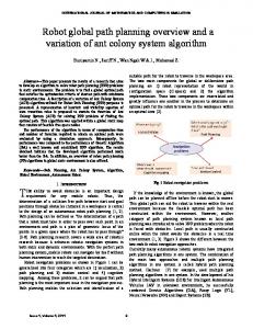
Fig. 1. Basic modules of the robot motion planning system.

109

110


choice for web-based applications by eliminating the need for porting programs to different platforms. Another key feature of Java is its support for distributed computing. Unlike most other programming languages, that rely on platform-dependent add-on utilities to support distributed computing, Java provides built-in language constructs and special APIs for distributed computing. We chose Java to build our system as we are highly motivated by the fact that Java is the leading-edge object-oriented programming language. Developing the system using Java makes the resulting software truly portable across multiple machine architectures. In Section 2, we define the problem and introduce basic notation and definitions. The graphical user interface components are discussed in Section 3. Next, we introduce the working and configuration spaces. Section 5 describes the motion planning algorithm. Finally, simulation results are presented in Section 6 before the work is concluded in Section 7. 2. Problem definition and preliminaries Motion planning has been regarded as a core algorithmic problem in computational robotics for many years, and many researchers have worked on finding better algorithmic solutions. The study of algorithms related to robot motion planning forms a major subarea of computational geometry. Motion planning is useful not only for computer control of actual robots; it is also useful in many areas such as assembly planning and computer animation. Motion planning refers to the computational process of moving from one place to another, in the presence of obstacles. The degree of difficulty of motion planning varies greatly depending on two factors: the first is whether all information regarding the obstacles (i.e. sizes, locations, motions etc) is known before the robot moves. The second is whether these obstacles move around, or stay in place as the robot moves. The simplest scenario, and the most researched and understood one, is in the case when all obstacles are static, and all details about these obstacles are known before path planning takes place. The problem for the robot, which is known as the motion planning problem, can be informally stated as getting from a starting point to an ending point, without colliding with any obstacle. The goal of the robot motion planning problem is to design autonomous robots that can be asked to move to a specific location without specifying how to go there. Such a robot should have sufficient information to decide how to reach its destination. Before we attempt to solve this problem, the following assumptions are set. (1) Two-dimensional environment: we assume a 2D planar region. (2) Convex shapes: this assumption is made to simplify our treatment of the problem. Non-convex shapes are not allowed and as a result, if the user specifies one, the system will automatically compute the convex hull and consider it as the shape. (3) Static environment: the robot is the only moving object in the environment. Before we proceed, we introduce the following basic definitions.


111

2.1. Work space and configuration space The work space (W-Space) is the space where the robot actually moves around: that is, the real world. The configuration space (C-Space) is the parameter space of the robot. Any convex robot in the work space is mapped to a point in the configuration space, and any point in configuration space corresponds to some placement of an actual robot in the work space. Figs. 4 and 5 show a working space and its C-Space, respectively. Notice the obstacles are grown by the robot’s size (light shaded areas surrounding them) and the robot is mapped to a point. This mapping transforms the problem of planning the motion of an object into the problem of planning the motion of a point. 2.2. Free space and forbidden space The free space is the space which is not occupied by obstacles in either W-Space or C-Space. For example, this corresponds to the white areas in Figs. 4 and 5. On the other hand, the forbidden space is the space occupied by obstacles, and it corresponds to the shaded areas in both figures. 3. Graphical user interface The set of general classes involved in the system is shown in Figs. 2 and 3. In order to perform the computation of the shortest collision-free path (connecting the starting point and the ending point), we need to go through a specific number of phases. First of all, we create the working environment using a variety of tools. The user may manipulate (move, resize and delete) any of the created shapes. However, the goal, which is an object, can only be either deleted or moved. The next step is to map obstacles from the working space into the configuration space. This is done using the Minkowski sum algorithm. This step is responsible for mapping the robot to a point in the configuration space after growing all obstacles by the size of the robot. The result will lead to computing the shortest collisionfree path, if one exists. Several other algorithms are described in Section 4. 3.1. Design phase Whether you aspire to develop the next big software hit or simply create computer applications for your personal use or office use, your applications need effective user interfaces. Designing such an interface involves discipline (following good design principles), science (usability testing) and art (creating screen layouts that are informative, intuitive and visually pleasing). Therefore, the graphical user interface (GUI) is firmly established as the preferred user interface for end users in most situations. Java provides an extensive framework for building high-quality graphical user interfaces (GUI). This framework is part of the Java foundation classes (JFC). The abstract windows toolkit (AWT) package provides the basic support for building graphical user interfaces. The Swing package is an extension of AWT, which provides rich support for building sophisticated-looking and high-quality interfaces. Swing components extend the AWT functionality by adding advanced, highly customizable components as well as control of the look and feel of the entire application. A major difference between the AWT

112


Fig. 2. Drawing canvas classes.

Fig. 3. Class hierarchy of the robot motion planning system.

components and the Swing components is the fact that most of the Swing components are lightweight whereas the AWT components are heavyweight. That is, Swing components avoid the overhead with the underlying platform and enforce a common look and feel. 3.2. Interface components Fig. 3 shows all classes involved in the implementation of this system. The graphical user interface (GUI) consists of the following.


113

3.2.1. Drawing canvas This region is used to set up the working space or environment (W-Space): that is, create the obstacles and the robot, choose goal point, set environment parameters and view the results. The upper region of Fig. 4 shows an example of a working space where obstacles (dark shaded shapes) and the robot (leftmost object) are created besides specifying the goal position (“+” sign). Mouse and keyboard event handlers are registered with this region. The drawing canvas is developed as a double-buffered canvas for smooth drawing and mouse/keyboard event handling. To create this blank space for drawing, we extend the JComponent class. The main fields of the canvas class are an image object and a graphics context associated with the image. The main methods in the class are paint() and update() which copy the image to the screen. An overridden method of repaint() is used to repaint only the rectangular area where a change takes place. This method is used to enhance the efficiency of drawing and improves its performance. The drawing canvas class overrides the method setBoundes() from the JComponents class. It is invoked by the Java GUI framework before the component first becomes visible and whenever the component is resized. This method is used in the drawing canvas class to set up its image object where it is copied to the new image whenever the canvas is resized so the drawings can be preserved. 3.2.2. Control panel This is the tools area, which is located below the drawing area, and contains all the necessary tools or control components to help in setting up the environment: that is, drawing and manipulating all objects. All available tools in the control panel are shown in the lower region of Fig. 4. The tools in the control panel are represented by the following Swing components: JButtons, JComboBoxes and JSliders. These components are part of the rich set of Java GUI framework classes, called GUI widgets. Widgets are the building blocks of the visual aspect of GUIs. Each widget class defines a particular type of widget by its visual characteristics (the look) and its behavior pattern in response to user input (the feel). The above GUI tools are encompassed in a lightweight JBox container. It uses the JBoxLayout layout manager. The control panel contains tools to choose obstacle/robot type, modify path resolution, specify safety parameter, compute the configuration space and generate and animate motion along a path. We allow circular, elliptical, rectangular and polygonal shapes which is a unique feature of our system when compared to other existing systems. The safety parameter determines how close the robot can be to an obstacle boundary while following its path. Notice that a safety value of 0 allows the robot to touch obstacles at the boundary. In order to activate these two main components, a drawing pad has been created. The drawing pad is implemented as both an application and an Applet. The classes used in the implementation of the canvas are shown in Fig. 2. The shaded classes are the ones that have been implemented; the rest are classes and interfaces of the Java Class Library. A user can select, delete, move and resize any object in the environment directly via the mouse. In addition, the user may choose to move objects using the arrow keys. A user needs only to select an object by pressing on it and then s/he can easily apply the desired operations. Such features distinguish our interface from other interfaces that require more effort to achieve similar functionalities.

114


Fig. 4. A sample of a working space/environment (W-Space). An animation of robot motion along the shortest path is shown with a safety value of 4.

4. Working and configuration spaces Objects (e.g., both the obstacles and the robot) are drawn using the press–drag–release combination of mouse events in the drawing canvas and are handled using Java mouse event listeners. Such a listener simply delegates the control of mouse-button presses, releases and mouse dragging of the current shape to the proper event handler. Although the shapes supported by the system have little in common, the ways in which they are drawn are quite similar. Each of the rectangular, elliptical or circular shapes is defined by two points (the two diagonally opposite corners). The desired drawing behavior is carried out by the press–drag–release combination. • When the mouse button is pressed, the current position of the mouse marks the first corner. • While the mouse is dragged, the bounding frame (referred to as the handle) of the selected shape is drawn. • When the mouse is released, the current position of the mouse identifies the second opposite corner of the selected shape. Upon releasing the mouse, the actual shape is drawn. These steps can be used to draw objects of any shape from the various available ones. Whenever the mouse moves over any object in the drawing canvas, this object is highlighted as a signal to the user of being ready for selection and then manipulation. When an object is selected, a user can easily drag it or move it by the arrow keys. A user can also resize a selected object by dragging any of the four corners of the handle. The listener interface for the keyboard events in Java is KeyListener. A selected object may be deleted by pressing the key. We have overridden all of the MouseListener and


115

MouseMotionListener classes’ methods to handle the various environment manipulation tasks by the mouse: for instance, methods mousePressed() and mouseReleased() (drawing, selecting), mouseDragged() (drawing, moving, resizing), mouseEntered() and mouseExited() (signals entering and exiting from the canvas) and mouseMoved() (highlighting shapes when mouse moves over it). While obstacles may overlap with each other, the system forbids the robot to overlap (collide) with any obstacle. Collision is an important issue that arises and requires computing the intersection of two shapes. When the user chooses a goal point, this point represents the reference point of the robot, which maps to be the left-bottom corner of the geometric shape of the robot. The new location of the goal may be rejected if the area surrounding it can not accommodate the robot. This type of verification, at this early stage, helps in eliminating undesirable degenerate cases, which must be dealt with at a later stage in the path planning process. Notice that the Goal button is enabled upon the creation of the robot. The objects’ geometric shapes should be maintained convex. Thus, a validation module is implemented to check for convexity of drawn objects. If a non-convex (i.e., concave) object is created, the module fixes it by computing the object’s convex hull. Its use is an acceptable assumption and has been widely used in the literature. Next, we present the algorithm for computing the convex hull, called Graham’s scan [1]. Algorithm ConvexHull(P) Input: A set P of vertices for an object Output: A list containing the vertices of CH(P) in CW order 1. Sort the points by x-coordinate, resulting in a sequence p1 , . . . , pn 2. Put p1 and p2 in a list Lupper 3. for i ← 3 to n 4. do Append pi to Lupper 5. while Lupper has more than 2 points and the last 3 points do not make right turn 6. do Delete the middle of the last 3 points from Lupper 7. Put the points pn and pn−1 in a list Llower 8. for i ← n − 1 downto 1 9. do Append pi to Llower 10. while Llower contains more than 2 points and the last 3 points do not make right turn 11. do Delete the middle of the last 3 points from Llower 12. Remove the first and last points from Llower to avoid the duplication where the upper and lower hull meet 13. Append Lupper to Llower , and call the resulting list L 14. return L We first compute the convex hull vertices that lie on the upper hull, which is the part of the convex hull running from the leftmost point p1 to the rightmost point pn when the vertices are listed in a clockwise order. In a second scan, which is performed from right to left, we compute the remaining part of the convex hull, the lower hull. Due to the sorting step, the total time required for computing the convex hull is O(n log n). This is one implementation of many others that have the same time complexity.

116


Fig. 5. Computing the C-Space and the visibility graph of the W-Space of Fig. 4.

All objects in the environment are maintained in a vector called shapesVector. The Java class Vector provides the capabilities of array-like data structures that can dynamically resize themselves. This vector makes the input of the next phase. The configuration space (C-Space) is the parameter space of the robot. A robot in W-Space is represented by a point in C-Space, and any point in C-Space corresponds to some placement of an actual robot in the W-Space [11]. The underlying idea of C-Space is to represent the robot as a point called the reference point of the robot and map the obstacles into this space by growing their sizes by the size of the robot. The outer boundary of the W-Space is considered as an obstacle and is mapped into the C-Space by enlarging it as for other obstacles in the environment by the size of the robot. This mapping transforms the problem of motion planning into the problem of planning the motion of a point. To make this mapping possible, we use an efficient algorithm known as the Minkowski sum algorithm [5]. Minkowski sums are a useful mathematical tool in the motion planning problem. Notice that a very simple algorithm to compute the Minkowski sums of two convex polygons is to compute v + w for each pair v, w of vertices, with v ∈ P and w ∈ R. Next, the convex hull of all these sums is computed. The MinkowskiSums algorithm only looks at pairs of vertices that are extreme in the same direction, which makes it run in linear time. In this → algorithm, the notation angle ( p, q) is used to denote the angle that the vector − pq makes with the positive x-axis. In order to perform the required computation, the lists of vertices for any two convex polygons should be maintained in clockwise order, with the first vertex in both lists as the smallest y-coordinate (and smallest x-coordinate in the case of ties). The Minkowski sum algorithm runs in linear time, because at each execution of the repeat-loop either i or j is incremented. One can observe that any vertex of the Minkowski sum is the sum of two original vertices that are extreme in a common direction, and the angle test ensures that all extreme pairs are found. So, the Minkowski sums of two


117

convex polygons with n and m vertices, respectively, has O(n +m) time complexity. Fig. 5 shows the output of the Minkowski algorithm for a translating robot (polygon—leftmost and topmost object in Fig. 4) (ignore the network of line segments for the time being). Notice how the robot is shrunk to its reference point (i.e., bottom left corner) whereas each obstacle including the outer boundary of the W-Space has been grown accordingly. Algorithm MinkowskiSums(P, R) Input: 2 convex polygons: P = {v1 , . . . , vn } and R = {w1 , . . . , wm }. The vertices follow a CCW order, where v1 and w1 are the smallest. Output: The Minkowski sums (P ⊕ R). 1. i = 1; j = 1 2. vn+1 = v1 ; wm+1 = w1 3. repeat 4. Add vi + w j as a vertex to P ⊕ R 5. if angle(vi vi+1 ) < angle(w j w j +1 ) 6. then i + + 7. else if angle(vi vi+1 ) > angle(w j w j +1 ) 8. then j + + 9. else i + + 10. j ++ 11. until i = n + 1 and j = m + 1 The resulting set of C-obstacles will be stored in another vector as it will be extensively used in the later phases. 5. Motion planning algorithms 5.1. The visibility graph The visibility graph of a set of obstacles is more complex. It is the graph of all nodes from all obstacles that can “see” each other. The edges formed must be external to the obstacles. It has been proven that visibility graphs guarantee to compute the shortest path because any shortest path between pst art and pgoal among the set S of disjoint polygonal obstacles is a polygonal path whose inner vertices are vertices of S. The above characterization of the shortest path enables us to construct the visibility graph of S, denoted by G vis (S). Its nodes are the vertices of S, and there is an arc between vertices v and w if they can see each other: that is, if the segment vw does not intersect the interior of any obstacle in S. Two vertices that can see each other are called (mutually) “visible”, and the segment connecting them is called a “visibility edge”. This also applies to the boundary—chain of line segments—of each obstacle. The endpoints of each boundary segment (edge) are visible to each other. Hence, the obstacle edges form a subset of the arcs of G vis (S). The segments on the shortest path are visibility edges, except for the first and the last segment. To make them visibility edges as well, the start and goal positions are added as vertices to S; that is, the visibility graph will be considered of the set S ∗ = S ∪ { pst art , pgoal }. By definition, the arcs of G vis (S ∗ ) are between vertices (which now include pst art and pgoal ) that can see each other.

118


The visibility graph is implemented using the adjacency list approach. Adjacency lists are linked lists, one list per vertex, that identify the vertices to which each vertex is connected (i.e. the visible vertices to that vertex). All the vertices are stored in an object of ArrayList, which is a dynamic array-class in Java. It is similar to the Vector class. Each component of an ArrayList object, in the graph, contains a reference to a linked list of edge nodes. Each node has a numeric index, a weight and a reference to the next node in the adjacency list. Class AdjVertex encompasses these attributes. The general specification of the implemented graph includes boolean methods for checking whether the graph is empty (isEmpty()) or full (isFull()), and several methods to add vertices (addVertex(vertex)) and edges (addEdge(from, to, weight)) and to retrieve the vertices connected to a certain vertex (getToVertices(vertex)). Fig. 5 shows the visibility graphs in the C-Space. Next, we describe the general sketch of the algorithm to compute the visibility graph. Algorithm VisibilityGraph(S) Input: A set S of disjoint polygonal obstacles including pst art and pgoal . Output: The visibility graph G vis (S). 1. Initialize the graph G = (V, E) where V is the set of all vertices of the polygons in S and E = φ 2. for all vertices v in V 3. do W = VisibleVertices(v, S) 4. for every vertex w ∈ W , 5. do add the arc (v, w) to E 6. return G If we want to test the visible vertices from a vertex, p, we have to check the segment pw over all obstacles. We can use the information we get when we test one vertex to speed up the test for other vertices. This can be accomplished by treating the vertices in cyclic order while maintaining information that helps to decide on the visibility of the next vertex. Algorithm VisibleVertices summarizes this operation. It first sorts the vertices by the clockwise angle that the segment from p to each vertex makes with the positive x-axis. Vertices that have the same angle are treated in order of increasing distance from p. The running time of VisibleVertices is O(n log n). Because this method is to be applied to each of the n vertices of S in order to compute the entire visibility graph, the visibility graph algorithm has an O(n 2 log n) time complexity, where n is the total number of obstacle edges. However, this algorithm works only for disjoint convex polygonal shapes. In our system, this assumption is very restrictive since we allow obstacles to overlap. Therefore, we modified the algorithm to handle overlapping obstacles with O(n 3 ) time complexity in the worst case. 5.2. Shortest path computation Based on the visibility graph, the shortest path between pst art and pgoal is computed using Dijkstra’s algorithm [5]. Dijkstra’s algorithm requires that each arc in the graph is assigned a weight (the Euclidean distance of the arc connecting its incident vertices). Since Dijkstra’s algorithm is to be used to find the shortest path between two points, pst art and pgoal , we can stop the search process whenever the shortest path of pgoal is reached.


119

We use an auxiliary structure for storing vertices to be processed at a later stage. We want to retrieve the vertex that is closest to the current vertex, that is, the vertex connected with the minimum edge weight. If we consider minimum distance to be the highest priority, the perfect structure to be used is the priority queue (minimum-heap). Therefore, the algorithm utilizes a heap structure whose elements are the visible vertices (edges) with the distance from the starting vertex pst art as the priority. The elements on the heap are objects with three attributes: fromVertex, toVertex and distance. We use the class PathNode to represent such objects. The basic operations defined for the priority queue include enqueuing (enqueue(PathNade)) and dequeuing of objects (dequeue()), which returns the highest-priority element from the priority queue, as well as testing for an empty (isEmpty()) or full (isFull()) priority queue. The output of this algorithm is a list of vertex pairs (edges) showing the total minimum distance from start vertex to each of the other vertices in the graph, as well as the last vertex visited before the destination. Here is the general outline of the algorithm: Algorithm ShortestPath(Graph, pst art ) Input: G vis (S ∗ ) and the starting point pst art Output: A list of vertex pairs that forms the shortest path from pst art to every other vertex in the graph. 1. graph.ClearMarks() 2. Set the fromVertex and toVertex fields of a PathNode item to pst art 3. Set item.distance to 0 4. Enqueue item to priority queue (pq) 5. repeat 6. Dequeue an item from pq 7. if item.toVertex is not marked 8. then Mark item.toVertex 9. Save item to Path ArrayList 10. item.toVertex = item.fromVertex 11. item.distance = minDistance 12. Get vertexQueue of vertices adjacent from fromVertex 13. while more vertices in vertexQueue 14. do Get next v in vertexQueue 15. if v is not marked 16. then v = item.toVertex 17. item.distance = minDistance+ 18. graph.weightIs(fromVertex, v) 19. Enqueue item to pq 20. until pq becomes empty 21. return Path where the “.” means the OO object membership. After determining the shortest path, the robot can start navigating in the W-Space upon the user’s request. Robot motion along the trajectory will be shown at discrete steps as depicted in Fig. 4 or 6. The discrete step is controlled by the resolution parameter, which can be set by the user.

120


Fig. 6. The shortest path becomes different when the safety value is set to 5. Compare with Fig. 4.

6. Simulation results and assessment The system has been developed in Java. The AWT and Swing packages of Java provided a rich collection of platform-independent components to create the system’s graphical user interface and to handle mouse and keyboard events. Our system can run as an Applet or a stand-alone application. A user can easily set up or model a working environment via the control panel as in Figs. 4 and 6. Both figures have dark objects (obstacles), a robot (light grey—polygon), and a goal position (“+” sign). The computation of the C-Space is automatically displayed for each environment upon request from the user. Fig. 5 shows the C-Space of the environment in Fig. 4 (light shaded areas added to obstacles). This is a major computation before further processing is performed. As depicted in Fig. 1, the visibility graph, the output of Dijkstra’s algorithm and the shortest path are computed based on the computation of the C-Space. This output result is shown in Fig. 5 too (it is the network of line segments connecting some vertices, the start and the goal positions). Notice that, in actual simulations, different colors are used to indicate the output of each phase. Once the shortest path is determined, the robot starts navigating towards the goal in discrete steps as depicted in Figs. 4 and 6. The robot may touch obstacles’ boundaries while navigating towards its goal. Therefore, we added a new parameter, called safety, to control the clearance distance between the robot and any obstacle’s boundary. Touching is allowed when the safety value is set to 0 as can be noticed in both figures mentioned. Usually safety is a major concern in robot motion planning: how close shall we allow the robot to be to obstacles? Although it is a desirable feature, it could eliminate a possible short path. One can argue that this is a price for safety. But what if the robot could not find a path at all and reports failure, provided one exists. Since finding a path is our major concern, then the system will adaptively re-adjust the safety value such that a path


121

Fig. 7. Students’ assessment of the software. Overall average is 4.39 out of 5.

is found. Fig. 4 shows a simulation where the shortest path is reported under a clearance value = 4. Fig. 6, on the other hand, shows a new shortest path, for the same environment as Fig. 4, after increasing the safety value to 5. This is because the previous shortest path, among others, is eliminated from the visibility graph and, as a result, the system reports the currently optimal one. The proposed software system was appraised by junior, senior and graduate students (35 students in total). Their comments provided useful feedback for improvement. The appraisal was intended to investigate a number of key issues regarding the value of the software as a Java-based CAL package for teaching purposes, which covers content, presentation, effectiveness, suitability to audience, ease of use and interaction with the interface. Results confirmed that the program is an extremely useful tool for teaching and learning the graph structure and its algorithms. Students also showed a great deal of satisfaction with the presentation, user interface and its ease of use. The outcome of this assessment is depicted in Fig. 7. We intend to further evaluate this system over the next two semesters before we accommodate any major changes, if any. We believe that using Java in developing this system, with the enormous collection of Java components, helped substantially in presenting complex modules in a more dynamic and interactive manner. The use of Java as a language along with its desirable GUI support provides a representation that is often better in communicating a concept than a static figure or a written description. It also helps the students to visualize the basic concepts, whenever possible, easily. Instructors can also gain by using such a tool. It will not only save their time and effort but will also bring more realism to the subject matter by providing real-time simulations. This system creates an interactive environment of learning by experimentation. As a result, such systems can increase motivation, instil greater interest among students and encourage them to be more actively involved in the classroom. 7. Conclusion Motion planning has been studied for several decades, and many motion planning algorithms have been presented. Therefore, research in robot motion planning remains one

122


of the important fields of study in the task of building robot systems. Computation of a collision-free path for a movable object (robot) among static obstacles is a fundamental subject in the fields of robotics. It involves mapping obstacles from the working environment into the configuration space, constructing the visibility graph and computing the shortest path. We have presented a system, developed in Java, to trace visually the output of each phase while computing the shortest path between two given points. The system has been developed in Java. We chose Java because we want to make this system accessible from the Internet. Such a system can be effectively used in a computerassisted learning environment. References [1] A.M. Andrew, Another efficient algorithm of convex hulls in two dimensions, Information Processing Letters 9 (1779) 216–219. [2] P. Backs, G. Tharp, K. Tso, The web interface for telescienec (wits), in: Proc. 1997 IEEE Int. Conf. on Robotics and Automation, Albuquerque, NM, 1997, pp. 411–417. [3] R. Breu, S. Hellebrand, M. Welzl, Experiences from teaching software development in a java environment, in: Proceedings of the Workshop on Practice and Experience with Java Programming in Education, Tunis, Tunisia, 2003, pp. 1–6. [4] J. Cruz, B. Cuesta, M. Sigut, L. Acosta, Simulation, remote access, and monitoring of a robot in java, International Journal of Robotics and Automation 17 (3) (2002) 112–119. [5] M. de Berg, M. van Kreveld, M. Overmars, O. Schwarzkoph, Computational Geometry: Algorithms and Applications, Springer-Verlag, Berlin, 2000. [6] S. George, Computer-supported collaborative learning in educational robotics, in: Proc. of the Ninth International Conference of AI in Education, LeMans, France, 1999, pp. 56–77. [7] S. George, P. Leroux, Project-based learning as a basis for a cscl environment: an example in educational robotics, in: Proc. of First European Conference on Computer-Supported Collaborative Learning, Maastricht, Netherlands, March, 2001, pp. 269–276. [8] K. Goldberg, M. Mascha, S. Gentner, N. Rothenberg, C. Sutter, J. Wiegley, Desktop teleoperation via the world wide web, in: Proc. of IEEE Int. Conf. on Robotics and Automation, Nagoya, Japan, 1995, pp. 654–659. [9] L. Jin, Y. Guo, Interactive piano mover live on www, Available online: http://www.cs.caltech.edu/∼ lei/cs20/c/project/src/pm.html (last accessed, 2003). [10] J. Latombe, Soccer simulator, 2000, Available online: http://robotics.stanford.edu/∼ latombe/cs326/2000/MotionPlanningInterface/. [11] T. Lozano-Perez, Spatial planning: A configuration space approach, in: Proc. of IEEE Trans. Comput. C-32, 1983, pp. 108–120. [12] S. Lynch, K. Rajendran, D. Parsons, Modeling gui interaction events for java learners, in: Proceedings of the Workshop on Practice and Experience with Java Programming in Education, Tunis, Tunisia, 2003, pp. 20–23. [13] H. Magno, J. Sethian, Java applet for robotic navigation with constraints, 1998, Available online: http://math.berkeley.edu/∼ sethian/Applets/java files robotic illegal/robotic illegal.html. [14] M. Overmars, Motion planning game, 2000, Available online: http://www.cs.uu.nl/∼ people/markov/kids/motion/index.html. [15] M. Rohrmeier, Interactive robot manipulation with vrml 2.0, 1998, Available online: http://www.robotic.dlr.de/STUDENTS/Martin.Rohrmeier/robot/robot.html. [16] K. Thramboulidis, An assignment-based approach to teach the object-oriented programming paradigm, in: Proceedings of the Workshop on Practice and Experience with Java Programming in Education, Tunis, Tunisia, 2003, pp. 7–14. [17] M. Xia, M. Wang, Global motion planning software, Available online: http://www.duke.edu/∼ msw7/Motion/Final.html (last accessed, 2003).