Oct 24, 2010 - [9] T. Aysal, M. Coates, and M. Rabbat, âDistributed average consensus ... [10] N. Michael, M. Zavlanos, V. Kumar, and G. Pappas, âDistributed ...
1
A gossip-based algorithm for discrete consensus over heterogeneous networks Mauro Franceschelli, Alessandro Giua, Carla Seatzu
Abstract Quantized consensus assumes that the state of each node may only take nonnegative integer values. Reaching consensus under quantization is equivalent to determining a balanced assignment of identical tasks to nodes. In this paper we generalize this problem in two ways and denote the resulting framework discrete consensus. First, we consider tasks that are not identical: each one is characterized by its own weight. Secondly, we assume that nodes are not identical as well. As an example, in the case of task assignment, that we consider as a reference problem in this framework, nodes may have different speeds and should be assigned a total weight proportional to their speed. We provide a gossip-based distributed algorithm that aims to minimize the maximum execution time over nodes, whose convergence to a bounded set is guaranteed. We show that the convergence time of the proposed algorithm relies ultimately on the average meeting time between two agents performing a random walk on a graph.
Published as: M. Franceschelli, A. Giua, C. Seatzu ”A gossip-based algorithm for discrete consensus over heterogeneous networks” IEEE Tran. on Automatic Control, Vol. 55, No. 5, pp. 1244-1249, May 2010.
This work has been partially supported by the European Community’s Seventh Framework Programme under project DISC (Grant Agreement n. INFSO-ICT-224498) M. Franceschelli, A. Giua and C. Seatzu are with Dip. di Ingegneria Elettrica ed Elettronica, Universit`a di Cagliari, Italy, {mauro.franceschelli,giua,seatzu}@diee.unica.it October 24, 2010
DRAFT
2
I. I NTRODUCTION The study of consensus networks has recently stirred much interest in the control community with a particular focus on the deep connection between consensus and algebraic graph theory [1]–[6]. In several applicative domains related to consensus the assumption that the state of each node is a continuous variable is clearly an oversimplified assumption, and it is necessary to explicitly take into account its discrete nature. This defines a new framework called quantized consensus [7]–[9] where the state only takes nonnegative integer values. It has been observed in [8] that reaching a consensus under this quantization constraint is equivalent to determining a balanced assignment of identical tasks to nodes. We generalize this approach, assuming that the tasks to be assigned to nodes may not be identical. Thus we assume that the state of each node is not described by an integer number, but by a collection of objects each one with its own integer weight. We call this framework discrete consensus. One of the most important classes of problems that can be formulated in terms of discrete consensus is given by task assignment. Tasks may be generic objects, e.g., spatial locations, network resources, or classifications. In particular, recent advances in communication and computation have allowed efficient solutions to the problem of task assignment [10]. Both online [11], [12] and off-line [13] approaches have been proposed: on-line approaches keep into account the variations of the task environment, while off-line approaches assume that the task environment keeps constant thus a solution can be computed in advance. Processor assignment and computation of an optimal execution sequence for multiversion software is an example of this kind of problems [14]. In this paper, that is a journal version of [15], we will focus on a problem of discrete consensus over heterogeneous networks. To provide a more intuitive interpretation to the considered physical variables, our problem formulation will be given in terms of task assignment although the approach is general. We assume that a given set of tasks, that may have different weight, should be assigned to agents (nodes). Networks are denoted as heterogeneous because nodes may have different speeds. The consensus problem for this type of nets, as far as we know, has not received much attention in the control literature. Our goal is that of determining, using consensus algorithms based on gossip [8], [16], the solution that minimizes the maximum execution time over nodes. It is based on the recent work
October 24, 2010
DRAFT
3
by Kashyap et al. [8] and on our previous results in [17] where homogeneous networks have been considered. Note that due to the discrete nature of tasks and to the assumption that tasks may have arbitrary weights, the optimality of the solution is not guaranteed. As discussed in [17] this is not related to our particular approach but is intrinsic in the nature of gossip, that implements at each step a pairwise optimization, and does not always yield an optimal solution. However, we prove that there exists a bounded set that contains the optimal solution that is always reachable and we study the convergence properties and the convergence time to this bounded set. As mentioned in the literature [8], [17], in the case of discrete consensus to ensure good convergence properties it is necessary to enrich the gossip algorithm with an appropriate swapping rule. Whenever a balancing between two nodes is not possible, the swap “shakes” the network configuration to redistribute the load and allows loads composed by discrete tasks to travel in the network, reaching a situation in which a new balancing may occur. When swaps are performed, the maximum average convergence time depends on the average meeting time of agents performing a random walk in a graph. We show that this can always be computed numerically, modeling the swap process with a Markov Chain with a single absorbing state that represents the meeting of the agents. We also discuss two particular net structures (fully connected networks and networks with ring topology) for which it is possible to compute the average meeting time analytically. II. P ROBLEM
STATEMENT
We consider a heterogeneous network of n nodes whose connections can be described by an undirected connected graph G = (V, E), where V = {1, 2, . . . , n} is the set of nodes and E ⊆ V × V is the set of edges. We assume that K indivisible tasks should be assigned to the nodes, and an integer weight cj , j = 1, . . . , K, is associated to each task. We define a weight vector c ∈ NK whose j-th component is equal to cj , and n binary vectors yi ∈ {0, 1}K such that: yi,j = 1 if the j-th task is assigned to node i, yi,j = 0 otherwise. To each node i ∈ V is allocated a load xi = cT yi consisting in the sum of the costs of tasks assigned to node i that must be processed.
October 24, 2010
DRAFT
4
The speed factor, denoted γi , represents the amount of load that can be processed in a time unit by node i. In the following we denote γmin the smallest speed in the network (clearly γmin > 0), and cmax the maximum weight of tasks in the network. The task assignment we are looking for is the one that minimizes the maximum execution time, starting from any initial condition. Namely, if we define the load and speed vectors h iT h iT and Γ = diag(γ), we would like to x = x 1 x 2 . . . x n , γ = γ1 γ2 . . . γ n minimize the following objective function: xi = kΓ−1 xk∞ i=1,...,n γi
f (x) = max
(1)
under the assumption that the total load remains constant, namely 1T x = 1T x(0), where x(0) represents the initial load configuration. Denoting Y (t) = [y1 (t) y2 (t) . . . yn (t)] the state of the network at time t, a centralized optimal solution to this problem can be determined solving the following integer programming problem with binary variables: T −1 min V = kc Y Γ k∞
s.t.
Y1=1
(2)
yi,j ∈ {0, 1} ∀ i = 1, . . . , n; j = 1, . . . , K.
We denote Y ∗ (resp., V ∗ ) the optimal solution (resp., the optimal value of the performance index) of Problem (2). III. G OSSIP ALGORITHM A. A distributed algorithm We first define a task exchange process between two adjacent nodes that, while not changing the value of the objective function, modifies the load configuration. Definition 3.1 (Swap): Let us consider two nodes i and r incident on the same edge. Let Ki (t), resp. Kr (t), be the set of tasks contained in node i, resp. r, at time t. Let us call swap the operation that moves the tasks in Ki (t) to r, and the tasks in Kr (t) to i at time t + 1, reaching the distribution Ki (t + 1) = Kr (t) and Kr (t + 1) = Ki (t), provided that
October 24, 2010
DRAFT
5
the objective function locally defined for the two nodes does not change, i.e., X µ c ¶ X µ c ¶ j j max , = γi j∈K γr j∈Ki(t+1) r(t+1) X µ c ¶ X µ c ¶ j j . max , γi j∈K γr j∈K i(t)
r(t)
¥ ˆ ir (t) = Ki (t) ∪ Kr (t) the set of tasks present in nodes i and r at time t. We We denote K ˆ ir (t) the projection of c on K ˆ ir (t), namely a vector whose elements are the define cˆ = c ↑ K weights of the tasks present in nodes i and r at time t. Using the same notation we define two ˆ ir (t) and yˆr = yr ↑ K ˆ ir (t), in other words each vector has a number binary vectors yˆi = yi ↑ K of elements equal to the number of tasks locally present in the nodes. Algorithm 1 (Gossip Algorithm with discrete tasks): 1) Let t = 0. 2) Select an edge {i, r} at random. 3) Solve the integer programming problem (IPP): k ∗ = min k cˆT yˆi s.t. ≤k γi cˆT (1 − yˆi ) ≤k γr k ∈ R+ ∪ {0}, ˆ yˆ ∈ {0, 1}|Kir (t)|
(3)
i
½
¾
cˆT yˆi (t) cˆT (1 − yˆi (t)) 4) If k < max , then γi γr let yˆi (t + 1) = yˆi and yˆr (t + 1) = 1 − yˆi , ∗
else execute a swap if possible. 5) Let t = t + 1 and goto step 2.
October 24, 2010
¥
DRAFT
6
1
=1
2
1
=1
2
3 3
Fig. 1.
=2
t
edge
0
node 1
node 2
node 3
V (Y )
4, 10
1, 2, 2, 3, 3, 5, 6, 7
14.5
1, 2, 2, 3, 3, 5, 6, 7
14.5
1
{1, 3}
4, 10
2
{2, 3}
4, 10
2,7
1,2,3,3,5,6
14
3
{1, 3}
5, 6
2, 7
1, 2, 3, 3, 4, 10
11.5
4
{2, 3}
5, 6
1, 2, 7
2, 3, 3, 4, 10
11
The network discussed in Example 3.2 and the results of Algorithm 1.
In practice IPP (3) provides the task assignment that minimizes the execution time at the two nodes. If the resulting assignment is better than the previous one, tasks are assigned accordingly, otherwise a swap is executed if possible. The swap allows to overcome several blocking conditions: anytime the network reaches a local minimum of the objective function the swap “shakes” the network ensuring convergence within some precise bounds (see Theorem 3.7). Example 3.2: Let us consider the fully connected1 net in Fig. 1 composed by 3 nodes with speeds γ1 = γ2 = 1 and γ3 = 2. Assume that it contains 10 tasks whose weights are equal to c1 = 1, c2 = c3 = 2, c4 = c5 = 3, c6 = 4, c7 = 5, c8 = 6, c9 = 7 and c10 = 10 and let the initial configuration be K1 (0) = {6, 10}, K2 (0) = ∅, K3 (0) = {1, 2, 3, 4, 5, 7, 8, 9}. Using Algorithm 1, we obtain the optimal task assignment in four steps, as summarized in the Fig. 1. In particular, the first line of the table summarizes the initial assignment to which it corresponds a value of the objective function that is equal to 14.5 (see the last column). The other lines point out the task assignment for t = 1, 2, 3, 4: in the second column we point out the selected edge, columns 3 to 5 point out the task assignment in the three nodes; finally, the last column points out the corresponding value of the objective function.
¥
B. Convergence properties The convergence properties of Algorithm 1 depend on the possibility of performing swaps.
1
A network is fully connected if there is an arc from each node to any other one.
October 24, 2010
DRAFT
7
1 γ1 = 1 5
γ1 = 1
γ3 = 2
γ5 = 3
2
3 γ4 = 2
7
6
γ7 = 3
γ6 = 3
4
(a) (1,4)
1
1 1
1
2
γ1 = 1
γ 2 = 1.1
1 1 1 3
(1,2)
(1,1) (2,4)
(2,3) (2,2) (2,1)
γ 3 = 1.2
(3,4) (3,3) (3,2)
(3,1) (b)
Fig. 2.
(1,3)
(c)
(a) The network discussed in Example 3.4: (b) Network in example 3.9 (c) A net with a generalized ring topology
where s = 3 and k = 4.
Definition 3.3 (Swap domain): We call swap domain Gγ ⊆ G a connected subgraph induced by nodes with the same speed.
¥
Example 3.4: Let us consider the network in Fig. 2.a that has seven nodes with three different speeds. This network can be partitioned in three different subgraphs G1 , G2 and G3 induced respectively by nodes {1, 2}, {3, 4} and {5, 6, 7}. In this case each swap domain is connected to each other.
¥
Each swap domain identifies a set of nodes where swaps may always happen. On the contrary swaps between adjacent nodes of different domains may either be possible or not, depending on the particular tasks and on the speed of nodes. As an example, if we consider the network in Example 3.2 a swap among nodes 1 and 3, that belong to different swap domains, is not allowed at time t = 1 because it would lead to an increasing of the maximum execution time at the two nodes. The following example shows a scenario in which a swap among nodes belonging to different swap domains is admissible. Example 3.5: Let us assume that two nodes 1 and 2 have speed equal to γ1 = 10 and γ2 = 11,
October 24, 2010
DRAFT
8
respectively. Moreover, let us assume that node 1 only contains one task of weight 10, while the second node contains two tasks both of weight equal to 5. The corresponding maximum execution time is equal to 1. Now, no tasks exchange may occur that leads to a better tasks assignment, while a swap may happen keeping unaltered the maximum execution time at the two nodes.
¥
It is relevant to note that the definition of “swap domain” is embedded in the graph topology: the nodes don’t need to know in which domain they are or even that any domain exists. Definition 3.6: We call final set Ye = {Y = [y1 y2 · · · yn ] |
¯ T ¯ ¯ c yi cT yr ¯ cmax ¯ ¯ ¯ γi − γr ¯ ≤ γmin ,
(4)
∀ i, r ∈ {1, . . . , n}} i.e., the set of configurations such that, for any couple of nodes i, r ∈ V , the difference among their execution times is at most equal to the ratio cmax /γmin .
¥
Theorem 3.7: Let Y (t) be the matrix that summarizes the task assignment resulting from Algorithm 1 at the generic time t. If each swap domain is connected to each other, it holds ³ ´ e denotes the probability that Y (t) ∈ Y. e limt→∞ Pr Y (t) ∈ Ye = 1 where Pr(Y (t) ∈ Y) Proof: We define a Lyapunov-like function V (t) = [V1 (t), V2 (t)]
(5)
consisting of two terms. The first one is equal to the objective function of (2), namely V1 (t) = kcT Y (t)Γ−1 k∞ . The second one is a measure of the number ¯ ¯ of nodes whose execution time is T ¯ ¯ c y (t) i ¯. equal to kcT Y (t)Γ−1 k∞ , i.e., V2 (t) = ¯¯arg max i=1,...,n γi ¯ Note that we impose a lexicographic ordering on the performance index, i.e., V = V¯ if V1 = V¯1 and V2 = V¯2 ; V < V¯ if V1 < V¯1 or V1 = V¯1 and V2 < V¯2 . The proof is based on three arguments. (1) We first prove that V (t) is a non increasing function of t. This is trivially true when a swap is executed, since in such a case V (t + 1) = V (t).
October 24, 2010
DRAFT
9
Consider the case in which the selected nodes i and r balance their load. It holds ½ T ¾ ½ T ¾ c yi (t + 1) cT yr (t + 1) c yi (t) cT yr (t) max , < max , , γi γr γi γr hence three different cases may happen. (a) One of the selected nodes is the only node in the network such that its execution time is equal to kcT Y Γ−1 k∞ . In such a case V1 (t + 1) < V1 (t) hence V (t + 1) < V (t). (b) One of selected nodes is such that its execution time is equal to kcT Y (t)Γ−1 k∞ but there exists at least one other node in the network with the same execution time. In such a case V1 (t + 1) = V1 (t) and V2 (t + 1) = V2 (t) − 1, hence V (t + 1) < V (t). (c) The execution time of both the selected nodes is smaller than kcT Y (t)Γ−1 k∞ . In such a case V (t + 1) = V (t). e then there (2) Secondly, we observe that, if the current configuration is outside the final set Y, exists at least one node whose execution time is equal to kcT Y (t)Γ−1 k∞ that could balance his load with (at least) one other node if they were incident on the same arc: this would reduce function V (t) (see cases (a) and (b) of the previous item). e then there To prove this we observe that if the current configuration is outside the final set Y, exists (at least) one couple of nodes i and r such that cT yi (t) cT yr (t) cmax − > γi γr min{γi , γr }
(6)
cT yi (t) is equal to the maximum execution time. If we move a task cj ≤ cmax from γi node i to node r we have: cT yi (t + 1) = cT yi (t) − cj , and cT yr (t + 1) = cT yr (t) + cj . Now where
cT yi (t + 1) cT yi (t) − cj cT yi (t) = < γi γi γi and
(7)
cT yr (t) cmax cT yi (t) cT yr (t) cj + ≤ + < γr γr γr min{γi , γr } γi
where the second inequality follows from assumption (6); thus cT yr (t) + cj cT yi (t) cT yr (t + 1) = < . γr γr γi
October 24, 2010
(8)
DRAFT
10
By (7) and (8) it follows that ½ T ¾ ½ T ¾ c yi (t + 1) cT yr (t + 1) c yi (t) cT yr (t) max , < max , . γi γr γi γr (3) Finally, we observe that being each swap domain connected to each other, there exists a series of swaps that lead to a configuration in which the loads of the two nodes identified in the previous item are adjacent and the arc between them is selected. This happens with probability 1 as t goes to infinity.
¤
Remark 3.8: Theorem 3.7 characterizes the convergence properties of Algorithm 1 in terms e This obviously does not imply that an optimal task assignment is achieved. of a finite set Y. As shown in [17] this is not a limitation of the particular algorithm. To reach consensus an optimization involving more than two nodes at the same time may be necessary.
¥
Finally the following example shows that if each swap domain is not connected to each other, then the convergence set Ye may not be reached by Algorithm 1. Example 3.9: Let us consider the network in Fig. 2.b where γ1 = 1, γ2 = 1.1, γ3 = 1.2. Tasks with cost c1 = c2 = . . . c6 = 1 are assigned such that K1 (0) = {1},
K2 (0) = {1, 1},
K3 (0) = {1, 1, 1}.
It can be seen that the network is in a blocking configuration where no task exchange may happen according to Algorithm 1. As a result the convergence set Ye is not reached being ¯ T ¯ ¯ ¯ ¯ c y1 cT y3 ¯ ¯ 3 ¯¯ cmax ¯ ¯ ¯ ¯ γ1 − γ3 ¯ = ¯1 − 1.2 ¯ = 1.5 > γmin = 1. On the other hand if node 3 and node 1 were connected, then node 3 could exchange one e task with node 1 and achieve a configuration included in Y. ¥ IV. C ONVERGENCE TIME OF A LGORITHM 1 The convergence time is a random variable defined for a given initial task assignment Y (0) = Y e Thus, Tconv (Y ) represents the number of steps as: Tconv (Y ) = inf {t | ∀ t0 ≥ t, Y (t0 ) ∈ Y}. required at a certain execution of Algorithm 1 to reach the convergence set Ye starting from a given tasks distribution. Let us firstly introduce the following notation.
October 24, 2010
DRAFT
11
•
Nmax is the maximum number of improvements of V (t) defined as in (5), needed by any e starting from a given configuration. realization of Algorithm 1 to reach the set Y,
•
Tmax is the maximum average time between two consecutive improvements of V (t) defined as in (5), needed by any realization of Algorithm 1, starting from a given configuration.
Using the previous notation, it follows that the expected convergence time is E[Tconv (Y )] ≤ Nmax · Tmax .
(9)
The following proposition provides a topology independent upper bound on Nmax . Proposition 4.1: Let us consider a net with n nodes and let γ be the corresponding speed vector. Let x(0) be the vector representative of the initial amount of load at nodes. It holds: Nmax ≤ (n − 1) · % · (M − m)
(10)
where n X
M = kΓ−1 x(0)k∞ ,
m=
xi (0)
i=1 n X
= γi
1T x(0) , 1T Γ1
(11)
i=1
% = max lcm{γi , γr }, {i,r}∈E
and lcm denotes the least common multiple. Proof: By definition the maximum number of improvements of V1 = f needed by any realization of Algorithm 1 to reach the set Ye is smaller or equal to the ratio between the global improvement of f needed before reaching the convergence set Ye starting from x(0), and its minimum admissible improvement. By Step 5 of Algorithm 1 the task assignment is updated if and only if leads to an improvement of the objective function, otherwise a swap is executed. Thus, the largest value of f (x) occurs at the initial configuration and is equal to M = f (x(0)) = kΓ−1 x(0)k∞ . The minimum value of f (x) corresponds to the case of perfect task assignment, that in general is not achievable in the discrete case. However, a lower estimate of it is given by its optimal
October 24, 2010
DRAFT
12
value in the case of infinitely divisible tasks, namely by f (x∗ ) where x∗ = αγ and α = Thus, if we define m = f (x∗ ) = α, then for any task assignment x it holds m ≤ f (x).
1x(0) . 1T Γ1
We also observe that the minimum load exchange is equal to 1 since all tasks have an integer weight. Now, if we consider the generic edge {i, r}, we know that the minimum improvement of f that we may obtain when balancing this edge is equal to 1/lcm{γi , γr }. As a consequence the minimum improvement of f at a generic step of Algorithm 1 is equal to 1/% = 1/ max{i,r}∈E lcm{γi , γr }, where E is the set of edges. Thus, we may conclude that the largest number of improvements of f before reaching the convergence set Ye starting from x(0) is at most equal to % · (M − m). Finally, in the worst case n−1 consecutive balancing may occur before having an improvement of f , namely n − 1 consecutive reductions of V2 may occur before having a reduction of V1 = f . In particular, this case may happen if n − 1 nodes have the same execution time that is equal to the maximum one. In this case, a first balancing may occur between the only “different” node and any of the other ones. Then, a new balancing may occur between any of the remaining n − 2 nodes with the maximum execution time and one with a smaller execution time, and so on. ¤ We now focus on Tmax . Evaluating Tmax , and hence the average convergence time (9), is in general a difficult issue because it is strictly related to the particular topology of the net. In the following we consider two cases: fully connected networks and generalized ring topology nets. Similar approaches based on Markov chains can always be used to evaluate numerically an upper bound on Tmax for a particular net example. A. Fully connected networks Proposition 4.2: Let us consider a fully connected network, and let n be the number of nodes. It holds Tmax =
n(n − 1) . 2
(12)
Proof: The maximum average time between two consecutive balancing occurs when only one balancing is possible. Thus, if N is the number of arcs of the net, then the probability of selecting the only arc whose incident nodes may balance their load is equal to p = 1/N , while October 24, 2010
DRAFT
13
the average time needed to select it is equal to N . Since the network is fully connected, if n is the number of nodes, the number of arcs is N = n(n − 1)/2 and so Tmax = n(n − 1)/2.
¤
Proposition 4.3: If a net is fully connected, the average convergence time of Algorithm 1 is E[Tconv (Y )] ≤ % · (M − m) ·
n(n − 1)2 = O(n3 ). 2
Proof: Follows from equation (9) and Propositions 4.1 and 4.2.
¤
B. Generalized ring topology Definition 4.4 (Generalized ring topology): A graph G = (E, V ) has a generalized ring topology if it satisfies the following assumptions. • It is composed by s rings, each one with k nodes. The generic j-th ring Rj is a graph Rj = (Vj , Ej ) with Vj = {1, . . . , k} and Ej = {{i, r} ∈ E | r = i+1, ∀i = 1, . . . , k−1}∪{k, 1}. • The same speed is associated to all nodes in the same ring, while nodes of different rings have different speeds. Thus each ring defines a different swap domain. • Let (i, j), with i = 1, . . . , k and j = 1, . . . , s, be the i-th node of ring Rj . Let Σi = {(i, j) ∈ V, j = 1, . . . , s} be the set of the nodes of index i in all rings. All nodes in Σi are fully connected, i.e., for all i = 1, . . . , k, there exists an edge in E that connects each node in Σi with any other node in Σi .
¥
An example of a net with a generalized ring topology is reported in Fig. 2.c: here s = 3, k = 4. Note that such a topology well fits with our problem for two main reasons. Firstly, it is scalable both in the number of nodes in the rings and in the number of rings (namely in the number of swap domains). Secondly, the diameter of the net, namely the maximum distance among nodes that may balance, increases with the number of nodes in the ring. Proposition 4.5: Let us consider a net with a generalized ring topology. Let s be the number of rings and n = k · s be the total number of nodes in the net. It holds ´ k 2 s(s + 1) n2 (s + 1) ³ n · + 16 = · (k + 16) . Tmax ≤ 32 · s s 32 October 24, 2010
(13)
DRAFT
14
Proof: We first observe that, due to the gossip nature of Algorithm 1 and to the random rule used to select the edges, the problem of evaluating an upper bound on Tmax can be formulated as the problem of finding the average meeting time of two agents walking on a graph executing a random walk. In fact, the average meeting time of the two agents may be thought as the average time of selecting an edge whose incident nodes may balance their load. Note that in general more than two edges may balance their load, thus assuming that only two agents are walking on the graph provides us an upper bound on the value of Tmax . In particular, the worst case in terms of meeting time occurs when the two agents are on different rings. In the following we compute the average meeting time using discrete Markov chains assuming that the two agents walk on different rings (worst case). For the sake of simplicity, we assume that the number of nodes k in each ring is even2 . We call distance between two agents in nodes (i, j) and (i0 , j 0 ), with j 6= j 0 , di,i0 = 1 + min{|i − i0 |, k − |i − i0 |}, namely the number of arcs in the shortest path connecting node i with node i0 . In simple words the above distance is equal to the distance between the two agents, computed as if they were in the same ring, plus 1 due to the fact that they are on different rings. This is consistent with the assumption that, in a generalized ring topology net, any node with a given index in a certain ring is connected to all the other nodes having the same index in different rings. Therefore nodes with a unitary distance are nodes within the same section Σ. Under the assumption that k is even, the maximum distance between the two agents is equal to D = k/2 + 1. The Markov chain relative to a net with an even value of k is shown in Fig. 3, thus it is a particular birth-death process. Each node (apart from the first one, named A) is characterized by an integer number that denotes the distance between the two nodes. Let us now discuss the weight of the arcs in the Markov chain. — The weight of the arcs going from nodes i to i + 1, and viceversa, for i = 2, . . . , D − 1 is equal to 2/N where N = ks(s + 1)/2 is the number of arcs3 . This follows from the fact that if a net has N arcs the probability of selecting a generic edge is equal to 1/N ; moreover, if the 2
The case of rings with an odd number of nodes k is upper bounded by the case of rings with k + 1 nodes.
3
The number of arcs of a ring topology net is equal to k times the number of arcs of each section Σ, plus k times the number
of arcs of each ring. Being each Σ a fully connected graph with s nodes, its number of arcs is equal to s(s − 1)/2. Therefore, N = ks(s + 1)/2 + ks = ks(s + 1)/2. October 24, 2010
DRAFT
15
distance between the two agents is i = 1, . . . , D − 1, two are the edges whose selection leads to an increasing or decreasing of their distance. The same reasoning explains the weight of the arc going from D − 1 to D and the weight of the arc going from 2 to 1. — If the distance between the two agents is unitary (the state of the Markov chain is 1) being by assumption the two agents on different rings, it means that they are on the same section. Two different cases may occur: either we select an edge that leads to a distance equal to 2, or the edge incident on the nodes containing the agents is selected. The first case occurs with a probability equal to 4/N ; the second case occurs with a probability equal to 1/N and leads to the absorbing state A. — Now, assume that the distance between the agents is equal to D. Since by assumption the two agents walk on different rings, in such a case the selection of 4 different arcs may lead to a decreasing of their distance. Therefore the arc of the Markov chain going from node D to node D − 1 has a weight equal to 4/N . — Finally, the weights of all self-loops are due to the fact that the sum of the weights of arcs exiting a node is equal to 1 in a discrete Markov chain. Given the Markov chain in Fig. 3 it is easy to compute the average hitting time of the absorbing state from any admissible distance. This can be done solving analytically the following linear system of equations: (I − P 0 ) τ = 1
(14)
where I is the D-dimensional identity matrix; P 0 has been obtained by the probability matrix P of the Markov chain in Fig. 3 removing the row and the column relative to the absorbing state4 ; τ is the D-dimensional vector of unknowns: its i-th component τ (i) is equal to the hitting time of the absorbing state starting from an initial distance equal to i, for i = 1, . . . , D; finally, 1 is the D-dimensional column vector of ones. We found out that the worst case in terms of hitting time occurs when the two agents are at their maximum distance, i.e., for i = D. In particular it ¡ ¢ 2 (s+1) k 2 s(s + 1) · ns + 16 = · (k + 16) where the last equality follows from the is τ (D) = n 32·s 32 fact that n = ks. This proves the statement being Tmax ≤ τ (D). ¤
4
It obviously holds that the hitting time of the absorbing state is null from the absorbing state itself.
October 24, 2010
DRAFT
16
1-5/N
1
2/N
1/N A
1
1-4/N 2/N
2 4/N
Fig. 3.
1-4/N
2/N
1-4/N 4/N D
3 2/N
2/N
2/N
The Markov chain associated to a generalized ring topology net with an even value of k.
Proposition 4.6: If a net has a generalized ring topology, then the average convergence time of Algorithm 1 in terms of the number of nodes n is E[Tconv (Y )] ≤
´ n2 (s + 1) ³ n · + 16 · (n − 1) = O(n4 ) 32 · s s or, in terms of the net parameters k and s % · (M − m) ·
E[Tconv (Y )] ≤ k 2 s(s + 1) · (k + 16) · (k s − 1) = O(k 4 s3 ). 32 Proof: Follows from equation (9) and Propositions 4.1 and 4.5. % · (M − m) ·
¤ V. C ONCLUSIONS AND FUTURE WORK In this paper we introduced a framework denoted as discrete consensus, that is a generalization of quantized consensus. We assumed that a set of tasks of different weight should be assigned to nodes with different speeds with the aim of minimizing the maximum execution time. A solution based on gossip has been proposed and convergence properties have been examined in detail. Future research in this topic will focus on determining appropriate rules to execute swaps to improve the convergence properties of Algorithm 1 and provide a stop criterion when the optimality set is reached. Finally, we plan to study the effects of delays in communication that often occurs in real applications. R EFERENCES [1] R. Carli, F. Fagnani, A. Speranzon, and S. Zampieri, “Communication constraints in the average consensus problem,” Automatica, vol. 44 (3), pp. 671–684, 2008. October 24, 2010
DRAFT
17
[2] A. Jadbabaie, J. Lin, and A. S. Morse, “Coordination of groups of mobile autonomous agents using nearest neighbor rules,” IEEE Trans. Automatic Control, vol. 48, pp. 988 –1001, 2003. [3] M. Ji, G. Ferrari-Trecate, M. Egerstedt, and A. Buffa, “Containment control in mobile networks,” IEEE Trans. on Automatic Control, vol. 53, pp. 65–78, 2008. [4] R. Olfati-Saber and R. M. Murray, “Consensus problems in networks of agents with switching topology and time-delays,” IEEE Trans. on Automatic Control, vol. 49, pp. 1520–1533, 2004. [5] W. Ren and R. Beard, Distributed consensus in multi-vehicle cooperative control. Theory and applications.
Springer
Verlag, 2008. [6] G. Xie and L. Wang, “Consensus control for a class of networks of dynamic agents,” Int. Journal of Robust and Nonlinear Control, vol. 17 (10-11), pp. 941–959, 2006. [7] R. Carli and S. Zampieri, “Efficient quantization in the average consensus problem,” Advances in Control Theory and Applications, pp. 31–49, 2007. [8] A. Kashyap, T. Bas¸ar, and R. Srikant, “Quantized consensus,” Automatica, vol. 43,7, pp. 1192–1203, 2007. [9] T. Aysal, M. Coates, and M. Rabbat, “Distributed average consensus with dithered quantization,” IEEE Trans. on Signal Processing, vol. 56, no. 10, pp. 4905–4918, 2008. [10] N. Michael, M. Zavlanos, V. Kumar, and G. Pappas, “Distributed multi-robot task assignment and formation control,” in Proc. 2008 IEEE International Conference on Robotics and Automation, Pasadena, California, May 2008. [11] K. Lerman, C. Jones, A. Galstyan, and M. Mataric, “Analysis of dynamic task allocation in multi-robot systems,” The Int. Journal of Robotics Research, vol. 25 (3), pp. 225–242, 2006. [12] M. Zavlanos and G. Pappas, “Dynamic assignment in distributed motion planning with local coordination,” IEEE Trans. on Robotics, vol. 24 (1), pp. 232–242, 2008. [13] M. Ji, S. Azuma, and M. Egerstedt, “Role-assignment in multi-agent coordination,” Int. Journal of Assistive Robotics and Mechatronics,, vol. 7 (1), pp. 32–40, 2006. [14] Y.-W. Leung, “Processor assignment and execution sequence for multiversion software,” IEEE Tran. on Computers, vol. 14 (12), pp. 1371–1377, 1997. [15] M. Franceschelli, A. Giua, and C. Seatzu, “Load balancing over heterogeneous networks with gossip-based algorithms,” in 2009 American Control Conference, St. Louis, Missouri, USA, Jun. 2009. [16] S. Boyd, A. Ghosh, B. Prabhakar, and D. Shah, “Gossip algorithms: design, analysis and applications,” in Proc. IEEE Infocom 2005, Miami, USA, Mar. 2005. [17] M. Franceschelli, A. Giua, and C. Seatzu, “Load balancing on networks with gossip based distributed algorithms,” in Proc. 46th IEEE Conf. on Decision and Control, New Orleans, LA, USA, Dec. 2007.
October 24, 2010
DRAFT