Aug 22, 2013 - We adapt the compression algorithm of Weinstein, Auerbach, and Chandra ... compressed SVD format, memory requirements are reduced.
Compression algorithm for discrete light-cone quantization Xiao Pu, Sophia S. Chabysheva, and John R. Hiller Department of Physics University of Minnesota-Duluth Duluth, Minnesota 55812
arXiv:1308.4911v1 [hep-ph] 22 Aug 2013
(Dated: August 23, 2013)
Abstract We adapt the compression algorithm of Weinstein, Auerbach, and Chandra from eigenvectors of spin lattice Hamiltonians to eigenvectors of light-front field-theoretic Hamiltonians. The latter are approximated by the standard discrete light-cone quantization technique, which provides a matrix representation of the Hamiltonian eigenvalue problem. The eigenvectors are represented as singular value decompositions of two-dimensional arrays, indexed by transverse and longitudinal momenta, and compressed by truncation of the decomposition. The Hamiltonian is represented by a rank-four tensor that is decomposed as a sum of contributions factorized into direct products of separate matrices for transverse and longitudinal interactions. The algorithm is applied to a model theory, to illustrate its use. PACS numbers: 11.15.Tk, 11.10.Ef, 02.60.Nm
1
I.
INTRODUCTION
The nonperturbative solution of quantum field theories generally requires numerical techniques. In Hamiltonian formulations, these typically take the form of matrix approximations to the eigenvalue problem for the mass eigenstates. The eigenstates themselves are represented by one-dimensional vectors with multiple indices, such as momentum components. If the Hamiltonian matrix elements are computed as needed and not stored in computer memory, the dominant memory requirement is the storage of these vectors. To possibly reduce this memory requirement, we wish to explore compression of these vectors. For the case of Hamiltonians for spin lattices, Weinstein et al. [1] have proposed a compression algorithm based on singular value decomposition (SVD) [2]. The lattice is split into two, and the eigenvectors |ψi become two-dimensional matrices indexed by the sublattices. A singular value decomposition reduces the matrix to a sum over contributions from individual sublattice vectors X λα |αi1 |αi2, (1.1) |ψi = α
where |αii is a vector on the ith sublattice and λα is the associated singular value of the original matrix. The sum over α is truncated to keep the nsvd largest contributions, thereby storing a compressed matrix as 2nsvd sublattice vectors. By doing all calculations in the compressed SVD format, memory requirements are reduced. There is, of course, a computational cost due to the extra processing. For diagonalization with a Lanczos-type iteration [3], the key step is multiplication of a compressed vector by the Hamiltonian, which must be done entirely within the SVD representation. The Weinstein algorithm includes this step. A standard technique for the nonperturbative solution of a quantum field theory is discrete light-cone quantization (DLCQ) [4, 5]. The theory is quantized in light-cone coordinates [6], which we take to be the light-cone time coordinate x+ = t + z and light-cone spatial coordinates x = (x− ≡ t − z, ~x⊥ ), with ~x⊥ = (x, y) being the transverse piece. Quantization in terms of these coordinates has the advantage of providing well-defined wave functions for eigenstates of the Hamiltonian [5]. The wave functions appear as coefficients in a Fock-state expansion of the eigenstate and are functions of the light-cone momenta pi = (p+ ~i⊥ ). The eigenstate |ψ(P )i has total momentum P and satisfies the i ≡ Ei + piz , p field-theoretic Schr¨odinger equation P − |ψ(P )i =
M 2 + P⊥2 |ψ(P )i, P+
(1.2)
where P − is the light-cone Hamiltonian, M is the mass of the state, and the expression given as the eigenvalue represents the mass-shell condition P − ≡ E + Pz = (M 2 + P⊥2 )/P + . The wave functions then satisfy integral equations obtained from this fundamental Schr¨odinger equation. The DLCQ approximation is roughly equivalent to a trapezoidal approximation to the integrals; the wave functions are represented by values at discrete momentum values and the Hamiltonian by a matrix. The vector that represents wave-function values is indexed by longitudinal and transverse momentum coordinates as well as other possible indices, such as flavor and spin. Therefore, it is easily re-interpreted as a multidimensional structure with many indices. By collecting these indices into two disjoint sets, instead of the one original set, the multi-ranked matrix becomes a rank-two matrix to which SVD can be applied. Here we propose a separation between transverse and longitudinal momenta. For the sample application that we use as 2
illustration, this is all that is needed. More generally, one can imagine including spin indices with transverse momenta and flavor indices with longitudinal momenta, to facilitate the factorization of the Hamiltonian. Angular momentum conservation in the z direction naturally pairs light-cone spin with transverse momentum in interactions, and flavor-dependent interactions in light-cone Hamiltonians commonly involve the constituent mass and longitudinal momenta. The SVD decomposition creates two sets of vectors, one with transverse index and one with longitudinal index, and the Hamiltonian matrix becomes a rank-four tensor. However, the Hamiltonian can be factorized as the sum of direct products of rank-two matrices, with one matrix indexed by transverse momenta and the other by longitudinal momenta. Thus, the Hamiltonian acts separately on the transverse vectors and longitudinal vectors. Because the factorization of the Hamiltonian typically has many terms, the outcome of multiplication by the Hamiltonian must be summed over many more contributions than in the original SVD decomposition and, therefore, must be compressed. This is where there is a significant computational load. However, this is the price to pay for reductions in memory requirements. In Sec. II we present the compression and diagonalization algorithms in some detail, both for completeness and to establish some notation. A sample application to a model theory is discussed in Sec. III. The results are summarized in the final section, Sec. IV. II.
ALGORITHM A.
SVD compression
We present the Weinstein compression algorithm [1] with expanded notation and in the context of the field-theoretic applications that we have in mind. The state vectors are Fockstate expansions, and each Fock state is factorized into a direct product of transverse and longitudinal states XX (2.1) Ain jn |vin i|wjn i. |ψi = n
in j n
The coefficients Ain jn are the discrete amplitude values at transverse momentum index in and longitudinal momentum index jn in the nth Fock sector. The in -jn Fock state has been factorized as |vin i|wjn i. In what follows, we combine all Fock sectors into the range of the indices, rather than keeping a separate sum over sectors, and drop the subindex n; however, in practice, the amplitudes Aij are compressed sector by sector, because the Hamiltonian acts only between neighboring sectors. The SVD decomposition of A can be written as [2] Aij =
NA X
λk Vik Wjk .
(2.2)
k=1
The P 2singular values λk are positive, decreasing in magnitude, and normalized to one: k λk = 1. The columns of V and W are orthonormal: X
Vik∗ Vik′ = δkk′ ,
X j
i
3
∗ Wjk Wjk′ = δkk′ .
(2.3)
The storage of the amplitudes is compressed by truncating the sum over k at nsvd < NA , keeping only terms with larger values of λk . The generic Hamiltonian H is factorized as a direct sum NH X
H=
α=1
(α)
(α)
(2.4)
(α)
(2.5)
HV ⊗ HW .
Its matrix elements in the factorized Fock basis are Hij,i′j ′ =
NH X
(α)
HV ii′ HW jj ′ ,
α=1
with
(α)
(α)
(α)
(α)
HV ii′ ≡ hvi |HV |vi′ i, HW jj ′ ≡ hwj |HW |wj ′ i.
(2.6)
Thus, although the matrix elements of H form a rank-four tensor, the tensor is decomposed into a set of rank-two matrices. The action of H on a state vector is to produce a new set of amplitudes NH nsvd X X (α,k) (α,k) vi wj , (2.7) A˜ij = k=1 α=1
with
(α,k)
vi
≡
p
λk
X
(α)
(α,k)
HV ii′ Vi′ k , wj
i′
≡
p X (α) λk HW jj ′ Wj ′ k .
(2.8)
j′
However, the new amplitude values are constructed from a sum over nsvd NH pairs of nonorthogonal vectors. The new vectors must be re-orthogonalized, and only the nsvd most important of them kept. This is the key step in the Weinstein algorithm [1], which we now describe in our notation. The new vectors are orthogonalized by application of SVD to the overlap matrices ′
′
hv (α ,k ) |v (α,k) i = (UV† DV UV )αk,α′ k′ and
′
(2.9)
′
† hw (α ,k ) |w (α,k)i = (UW DW UW )αk,α′ k′ ,
(2.10)
where UV and UW are unitary and DV and DW are diagonal. Notice also that the indices on the right-hand sides are reversed in order. Orthonormal vectors can then be formed as X −1/2 (α′ ,k ′ ) (α,k) = (DV UV )α′ k′ ,αk vi v˜i (2.11) α,k
and
(α′ ,k ′ )
w˜j
=
X
−1/2
(DW
(α,k)
UW )α′ k′ ,αk wj
.
(2.12)
α,k
Inversion of these sums recovers the original vectors X � † 1/2 � (α,k) UV DV vi =
αk,α′ k ′
α′ ,k ′
4
(α′ ,k ′ )
v˜i
(2.13)
and
(α,k)
wj
=
X � † 1/2 � UW DW
(α′ ,k ′ )
αk,α′ k ′
α′ ,k ′
w˜j
.
(2.14)
Substitution into the expression (2.7) for the new amplitudes yields XX (α′ ,k ′ ) (α′′ ,k ′′ ) w˜j , Cα′ k′,α′′ k′′ v˜i A˜ij =
(2.15)
α′ ,k ′ α′′ ,k ′′
with C
α′ k ′ ,α′′ k ′′
X � 1/2 � DV UV∗ = α,k
1/2
α′ k ′ ,αk
� � 1/2 UW DW
αk,α′′ k ′′
.
(2.16)
1/2
† As a rank-two matrix, C is just DV UV∗ UW DW , to which SVD can be applied, to obtain C = ULT Λ′ UR . Here Λ′ is diagonal with entries λ′n , again decreasing in magnitude. For matrix elements of C, we then have
Cα′ k′ ,α′′ k′′ =
nsvd NH X
ULT
n=1
�
α′ k ′ ,n
λ′n (UR )n,α′′ k′′ .
(2.17)
The sum over n is truncated to the first nsvd terms. Substitution into (2.15) then yields the compressed approximation to the amplitudes A˜ij ≃
nsvd X n=1
λ′n
X�
−1/2
UL DV
α,k
UV
�
n,αk
(α,k)
vi
X�
−1/2
UR DW
UW
α′ ,k ′
�
n,α′ k ′
(α′ ,k ′ )
wj
.
(2.18)
This brings the action of the Hamiltonian back to the compressed SVD form with nsvd terms. B.
Diagonalization
~ = λψ, ~ where the matrix H is not stored but inFor a matrix eigenvalue problem H ψ stead computed as needed, a natural choice for the diagonalization method is the Lanczos algorithm [3]. In the case of a complex symmetric matrix, such as will occur in the model discussed below, the algorithm generates a sequence of vectors {~un } from an initial guess ~u1 by the following steps: ~vn+1 = H~un − bn ~un−1 (with b1 = 0) an = ~vn+1 · ~un ′ ~vn+1 = ~vn+1 − an ~un q ′ ′ bn+1 = ~vn+1 · ~vn+1
(2.19)
′ ~un+1 = ~vn+1 /bn+1 .
The dot products do not use conjugation, which leaves an and bn possibly complex. The dot product between two vectors stored in compressed SVD form, such as Aij =
nsvd X
λk Vik Wjk and Bij =
nsvd X k=1
k=1
5
′ , λ′k Vik′ Wjk
(2.20)
can be written as ~ ·B ~ = A
nsvd X k,k ′
λk λk ′
X i
Vik Vik′ ′
X
′ Wjk Wjk ′.
(2.21)
j
These steps produce a complex symmetric, tridiagonal representation T of the original matrix, with an as the diagonal elements and bn the off-diagonal elements, with respect to the orthonormal vectors ~un . Diagonalization of T then provides the eigenvalues of H; if the iterations are stopped before a complete orthonormal basis is generated (which is usually the case), the eigenvalues of T approximate those of H, with the largest and smallest approximated best. The basis of Lanczos vectors ~un is orthonormal only if exact arithmetic is used in the computations. As is well known, round-off error will gradually destroy the orthogonality and allow copies of previous Lanczos vectors to enter the set, along with copies of eigenvalues in the diagonalization of T [3]. This de-orthogonalization is made much worse by SVD compression of the Lanczos vectors. Not only is each multiplication by H approximated through compression, as described in the previous subsection, but each subtraction of compressed vectors also requires an additional compression step, to keep the resulting vector at the same level of compression. The errors introduced by these compressions rapidly destroy orthogonality and render the Lanczos process useless. Instead, we use a power method with forced orthogonalization, as do Weinstein et al. [1]. From an initial guess ~v1 , a sequence of vectors ~vn = H~vn−1 is generated up to order n = b. This set of b vectors, all in compressed SVD form, is orthogonalized by applying SVD to the overlap matrix h~vn |~vn′ i, to obtain an orthonormal set {~u1 , ~u2, . . . , ~ub }. The matrix representation of H in this basis, Hij = h~ui |H|~uj i, is diagonalized. The smallest eigenvalue and its corresponding eigenvector are extracted, and the eigenvector is used as a new ~v1 to generate a new sequence. The process is repeated until the eigenvalue converges. The value of b is kept small, to minimize storage requirements for the sequence of vectors; for results reported here, we used b = 3.
III. A.
SAMPLE APPLICATION Model theory
As an illustration of the use of the compression and diagonalization algorithms, we apply them to the DLCQ approximation of a simple model. This model was previously considered by Brodsky et al. [7] without compression. They constructed the model as the light-front analog of the Greenberg–Schweber static-source model [8], designed to have an analytic solution. It can be viewed as a heavy-fermion limit of the Yukawa model, where the fermion has no true dynamics of its own and acts only as a source and sink for bosons, without changing its spin. 6
The light-cone Hamiltonian for the model is Z + X dp+ d2 p⊥ M02 − ′ p P = ( + + M0 + ) b†pσ bpσ 3 + 16π p P P σ � � Z 2 2 2 + 2 µ21 + q⊥ dq d q⊥ µ + q⊥ † † aq aq + a1q a1q + 16π 3 q + q+ q+ Z Z Z 2 2 dp+ dq + d2 q⊥ X † g dp+ 2 d p⊥2 1 d p⊥1 p p + + b bp σ P 16π 3 q + σ p1 σ 2 16π 3 p+ 16π 3p+ 1 2 � + �γ �� + �γ p2 p1 † aq δ(p1 − p2 + q) + aq δ(p1 − p2 − q) × + p2 p+ 1 � + �γ � � + �γ p2 p1 † +i + a1q δ(p1 − p2 + q) + i + a1q δ(p1 − p2 − q) , p2 p1
(3.1)
where b†pσ creates a fermion with momentum p and spin σ, a†q creates a boson with momentum q, and a†1q creates a heavy Pauli–Villars (PV) boson with momentum q. The PV boson is included to regulate the model at large transverse momenta [7, 9]. The subtractions necessary for the regularization are arranged by assigning an imaginary coupling to the PV boson. The bare mass of the fermion is M02 ; the term with M0′ is a counterterm needed to subtract against the fermion self-energy. The masses of the physical and PV bosons are µ and µ1 , respectively. With no fermion loops allowed, the boson masses are not renormalized. The parameter γ allows for a continuum of models; however, we consider only the most natural value, γ = 1/2, for which the small-momentum behavior of the wave functions is uniformly a square-root dependence. A mass eigenstate of this Hamiltonian, the one that represents the fermion dressed by a cloud of bosons, can be expanded in Fock states as |Φσ (P )i =
√
16π 3 P +
n1 Z n Z X Z dp+ d2 p⊥ Y drj+ d2 r⊥j dqi+ d2 q⊥i Y p p q 16π 3 p+ i=1 16π 3 qi+ j=1 16π 3 rj+ n,n1
×δ(P − p −
n X i
qi −
n1 X
n
r j )φ
j
(n,n1 )
(3.2) n
1 Y Y 1 † † (q i , rj ; p) √ bpσ aq a†1rj |0i. i n!n1 ! i j
Its normalization is hΦσ (P ′ )|Φσ (P i = 16π 3 P + δ(P ′ − P ),
(3.3)
which implies the following condition for the Fock-state wave functions: 1=
n Z XY n,n1
i
dqi+ d2 q⊥i
n1 Z Y j
2 X X r j ) . qi − drj+ d2 r⊥j φ(n,n1 ) (q i , rj ; P − i
(3.4)
j
We keep to a frame where the total transverse momentum P~⊥ is zero and the mass eigenvalue problem is M2 P − |Φσ (P )i = + |Φσ (P )i. (3.5) P 7
This leads to a coupled set of integral equations for the wave functions [7] "
M 2 − M02 − M0′ p+ − ( √
X µ2 + q 2
⊥i
i
yi �
−
2 X µ21 + r⊥j
zj
j
#
φ(n,n1 ) (q i , rj , p)
(3.6)
�γ p −q φ(n+1,n1 ) (q i , q, r j , p − q) =g n+1 p+ �γ 1 X p+ p +√ φ(n−1,n1 ) (q 1 , . . . , q i−1 , qi+1 , . . . , qn , rj , p + q i ) + + + 3 n i 16π qi p + qi � �γ Z √ dr + d2 r⊥ p+ − r + +i n1 + 1 √ φ(n,n1 +1) (q i , rj , r, p − r) r+ 16π 3 r + !γ + X i 1 p (n,n1 −1) q +√ φ (q i , r1 , . . . , r j−1, r j+1, . . . , r n1 , p + r j ) , + + n1 j 16π 3 r + p + rj Z
+ 2
dq d q⊥ p 16π 3 q + � 1
+
+
j
with yi = qi+ /P + and zj = rj+ /P + . There is an analytic solution φ
(n,n1 )
√ (−g)n (−ig)n1 √ = Z n!n1 !
�
p+ P+
�γ Y i
p
yi 16π 3 qi+ (µ2
2 + q⊥i )
Y j
q
zj 2 ) 16π 3 rj+ (µ21 + r⊥j
, (3.7)
with M0 = M and M0′ =
g 2 /P + ln µ1 /µ , 16π 2 γ + 1/2
(3.8)
which guided the earlier work [7]. The DLCQ approximation uses as a basis the discrete set of plane waves with (anti)periodic boundary conditions on the light-cone box − L < x− < L , −L⊥ < x, y < L⊥ .
(3.9)
The allowed momenta are then the discrete set p+ →
π π π ny ) , n , p~⊥ → ( nx , L L⊥ L⊥
(3.10)
with n even for bosons, corresponding to periodic boundary conditions, and n odd for fermions and antiperiodic boundary conditions. The total longitudinal momentum P + for the dressed fermion defines an odd integer K, called the resolution [4], such that P + = πK/L. The longitudinal momentum fractions are then all of the form n/K, and 1/K sets the longitudinal resolution of the approximation. Integrals are approximated by the trapezoidal rule Z
dp
+
Z
2π d p⊥ f (p , ~p⊥ ) ≃ L 2
+
�
π L⊥
�2 X n
8
N⊥ X
nx ,ny =−N⊥
f (nπ/L, ~n⊥ π/L⊥ ) .
(3.11)
This yields a matrix approximation for the coupled integral equations of the model [7] " n X µ2 + π 2 (m2ix + m2iy )/L2⊥ M 2 − M02 − M0′ − (3.12) K m /K i i # 2 2 X µ21 + π 2 (ljx + ljy )/L2⊥ − ψe(n,n1 ) (mi , lj , n) lj /K j ( X 1 � n − m �γ gπ √ √ ψe(n+1,n1 ) (mi , m, lj , n − m) = n m L⊥ 8π 3 m � �γ X 1 n + ψe(n−1,n1 ) (m1 , . . . , mi−1 , mi+1 , . . . , mn , lj , n + mi ) √ m n + m i i i � � γ X 1 n−l √ +i ψe(n,n1 +1) (mi , lj , l, n − l) n l l ) X 1 � n �γ p +i ψe(n,n1 −1) (mi , l1 , . . . , lj−1 , lj+1 , . . . , ln1 , n + lj ) , n + l l j j j
with n = K −
P
i
mi −
P
j lj ,
e(n,n1 )
ψ
K = (K, ~0⊥ ), and
" � � #(n+n1 )/2 2 p 2π π = n!n1 ! φ(n,n1 ) . L L⊥
The normalization of the discrete amplitudes ψe(n,n1 ) is 1=
XX n,n1 m1
P′
′
···
X X ′
mn
l1
′
···
X ln
1
′
e(n,n1 ) 2 ψ
N{mi } N{lj }
,
(3.13)
(3.14)
where the prime on the sum mi restricts the momenta m1 , . . . , mn to one ordering and where the factorials N{mi } ≡ Nm1 !Nm2 ! · · · , with Nm1 the number of times that m1 appears in the collection {mi }, take into account multiplicities of identical particles. We include these factors in the normalization rather than in the coupled equations, so that the Hamiltonian matrix can factorize between transverse and longitudinal momenta. B.
Results
In order to compute results, we must first have a finite matrix representation. At fixed resolution K, the matrix representation is finite in size with respect to the longitudinal momenta. This is because all longitudinal momenta are positive. For a state with bosons of longitudinal momentum P P indices mi , PV bosons with indices lj and fermion index n, K must equal n + i mi + j lj . All indices are positive, and therefore the range of the sums must be finite. Consequently, at fixed K the maximum number of bosons and PV bosons is finite. Results are calculated for K = 11 and 13, for which the maximum number of bosons in a Fock state is five and six, respectively. 9
For the transverse directions, we must impose a cutoff N⊥ on the range of transverse indices. The cutoff used in [7] was to limit the invariant mass of each particle: (µ2 +p2⊥ )/p+ < Λ2 . We cannot use such a cutoff here because it does not factorize between transverse and longitudinal momentum components. Instead we directly limit the range N⊥ of transverse indices. To keep the calculation small in size, we have used only N⊥ = 1 for physical and PV bosons, and N⊥ = 2 for the fermion. The total number of Fock states in the basis is then 23,046 for K = 11 and 89,739 for K = 13. Because we use a different cutoff, the numerical results can only be compared with Ref. [7] in the limit of infinite resolutions K and N⊥ . In this same limit we should recover the analytic answer. However, our purpose is to evaluate the compression algorithm, not DLCQ itself. Therefore, what we should check is whether there is convergence to a numerical result at a particular set of resolutions as the compression is removed, not whether the numerical result converges to the exact answer. The values used for the parameters of the model are taken from [7] at comparable resolutions. These values are M02 = 0.8547µ2 and g = 13.293µ for K = 11, and M02 = 0.8518µ2 and g = 13.230µ for K = 13. In both cases, µ21 = 10µ2 and L⊥ = 0.8165µ/π. The initial guess for the power method iterations was to set the bare fermion amplitude to one and all other wave functions to zero. The results for the smallest eigenvalue M 2 , as a function of the compression, are given in Fig. 1. As the compression is removed, the eigenvalue clearly converges. In Fig. 2, we show the percentage reduction in memory achieved at each level of compression. This reduction is defined as the ratio of the memory used for a compressed vector Mnsvd to that required for a standard one-dimensional array M1D : Θ=
Mnsvd × 100% M1D
(3.15)
At relatively coarse compressions of ∼ 70%, the eigenvalue differs from the converged value by ∼ 3%. In larger calculations, the compression ratio can be much smaller. In these tests, the value of the longitudinal resolution K is not particularly high and limits the number of longitudinal states in any one Fock sector to no more than 10 for K = 11 and 15 for K = 13. The number of transverse states is much larger, at 2917 and 9093, respectively. As K is increased, the amount of compression can be increased. IV.
SUMMARY
We have converted the Weinstein compression algorithm [1] to a form applicable to the DLCQ approximation [5] of a quantum field theory. As a test, we have applied it to a model theory [7] and investigated the effects of compression on convergence of the mass eigenvalue and on the memory requirements. The results are shown in Figs. 1 and 2. They indicate that in a larger calculation, of the sort required for good overall convergence, the memory savings could be substantial, at the small cost of a few percent in the accuracy of the answer. There is, of course, a significant increase in computational overhead. Also, these reductions in memory for vectors are only meaningful if the Hamiltonian matrix elements are computed as needed; when the Hamiltonian is stored, its memory requirements dwarf those of the vectors. 10
1.53 1.52
2
M /µ
2
1.51 1.50 1.49 1.48 1.47 0
2
4
6
8
10
nsvd FIG. 1. Mass eigenvalues M 2 as functions of the compression parameter nsvd . The DLCQ resolutions are K = 11 for the filled triangles and K = 13 for the filled squares. The masses are measured in units of the constituent boson mass µ.
The diagonalization method paired with the compression algorithm must be chosen carefully. Ordinary Lanczos iterations fail because they require vector subtractions, which can be computed only approximately for compressed vectors; the usual loss of orthogonality that occurs in the Lanczos method is greatly exacerbated by these errors. We instead used a power method combined with explicit orthogonalization, as suggested in [1]. This was sufficient to extract the smallest eigenvalue. This work could be extended in various ways. For the model considered here, additional tests could be done at larger values of K, if the Hamiltonian matrix is computed as needed, as it must be in a real application, rather than stored, which was done here for convenience. Theories in 2+1 dimensions, including a lower-dimensional version of this model, might be the more natural place for this algorithm, because having one less transverse dimension would bring the wave function matrices closer to the square shape that is optimal for compression. A first application to a real, (3+1)-dimensional theory would naturally be to Yukawa theory, where, unlike the present model, the fermion would have its own dynamics and the interactions would include spin. This could be compared with the uncompressed DLCQ approximation studied by Brodsky et al. [10]. 11
100
Θ(%)
90
80
70
0
2
4
6
8
10
nsvd FIG. 2. Same as Fig. 1, but for the compression ratio Θ. ACKNOWLEDGMENTS
This work was supported in part by the Department of Energy through Contract No. DE-FG02-98ER41087.
[1] M. Weinstein, A. Auerbach, and V.R. Chandra, Phys. Rev. E 84, 056701 (2011). [2] W.H. Press, S.A. Teukolsky, W.T. Vetterling, and B.P. Flannery, Numerical Recipes: The Art of Scientific Computing, (Cambridge, New York, 2007). [3] C. Lanczos, J. Res. Nat. Bur. Stand. 45, 255 (1950); J. Cullum and R.A. Willoughby, J. Comput. Phys. 44, 329 (1981); Lanczos Algorithms for Large Symmetric Eigenvalue Computations (Birkhauser, Boston, 1985), Vol. I and II. [4] H.-C. Pauli and S.J. Brodsky, Phys. Rev. D 32, 1993 (1985); 32, 2001 (1985). [5] For reviews of light-cone quantization, see M. Burkardt, Adv. Nucl. Phys. 23, 1 (2002); S.J. Brodsky, H.-C. Pauli, and S.S. Pinsky, Phys. Rep. 301, 299 (1998). [6] P.A.M. Dirac, Rev. Mod. Phys. 21, 392 (1949). [7] S.J. Brodsky, J.R. Hiller, and G. McCartor, Phys. Rev. D 58, 025005 (1998). [8] O.W. Greenberg and S.S. Schweber, Nuovo Cimento 8, 378 (1958). [9] W. Pauli and F. Villars, Rev. Mod. Phys. 21, 434 (1949). [10] S.J. Brodsky, J.R. Hiller and G. McCartor, Phys. Rev. D 64, 114023 (2001).
12