Nov 15, 2007 - William Frankel Center for Computer Sciences and the Israel Min- istry of Science and .... Moule, K., McCool, M.D.: Efficient bounded adaptive ...
Visual Comput (2008) 24: 139–153 DOI 10.1007/s00371-007-0180-1
Yotam Livny Neta Sokolovsky Tal Grinshpoun Jihad El-Sana
Published online: 15 November 2007 © Springer-Verlag 2007
Y. Livny (u) · N. Sokolovsky · T. Grinshpoun · J. El-Sana Department of Computer Science, Ben-Gurion University of the Negev, Beer-Sheva, Israel {livnyy, netaso, grinshpo, el-sana}@cs.bgu.ac.il
ORIGINAL ARTICLE
A GPU persistent grid mapping for terrain rendering
Abstract In this paper we present persistent grid mapping (PGM), a novel framework for interactive view-dependent terrain rendering. Our algorithm is geared toward high utilization of modern GPUs, and takes advantage of ray tracing and mesh rendering. The algorithm maintains multiple levels of the elevation and color maps to achieve a faithful sampling of the viewed region. The rendered mesh ensures the absence of cracks and degenerate triangles that
may cause the appearance of visual artifacts. In addition, an external texture memory support is provided to enable the rendering of terrains that exceed the size of texture memory. Our experimental results show that the PGM algorithm provides high quality images at steady frame rates. Keywords Terrain rendering · Graphics processors · Multiresolution hierarchies
CPU and graphics hardware often forms a severe transportation bottleneck. These limitations usually result in Interactive rendering of terrain datasets has been a chal- non-uniform or unacceptably low frame rates. Ray-tracing approaches generate quality images of lenging problem in computer graphics for decades. Terrain geometry is an important component of various visual- large terrain datasets by shooting rays from the viewpoint ization and graphics applications ranging from computer through the pixels of the viewport and computing their games to professional flight simulators. The need for accu- first intersection with the terrain surface. The values of rate visualization has led to the generation of large terrain final-image pixels are computed based on the color and datasets that exceed the interactive rendering capabilities normal at intersection points. In such a scheme, the renderof current graphics hardware. Moreover, the rendering of ing time is determined by the number of shot rays and the dense triangulations on the screen can cause undesirable complexity of computing the first intersection. To adopt aliasing artifacts. Since level-of-detail rendering manages this approach for interactive terrain rendering, one needs to decrease the geometric complexity and reduce aliasing to reduce the number of shot rays and to simplify or acartifacts, it seems to provide an appropriate framework for celerate computing of ray-terrain intersection. Reducing the number of shot rays may deprive some pixels from reinteractive rendering of large terrain datasets. Several level-of-detail approaches have been developed ceiving accurate values, which often causes unacceptable for interactive terrain rendering. Traditional multiresolu- image quality. Current graphics hardware provides common function and view-dependent rendering algorithms rely on the CPU to extract the appropriate levels of detail which are tionality for both vertex and fragment processors. This sent to the graphics hardware for rendering in each frame. functionality is useful for generating various effects [16], In these approaches, the CPU often fails to extract the such as displacement mapping and multitexturing. These frame’s geometry from large datasets within the duration significant improvements in graphics hardware necesof one frame. In addition, communication between the sitate the development of new algorithms and tech-
1 Introduction
140
Y. Livny et al.
niques to utilize the introduced processing power and programmability. In this paper, we present the persistent grid mapping (PGM) technique, a novel framework for interactive terrain rendering (see Fig. 1). Our algorithm takes a different approach from previous techniques and as a result, achieves a twofold advantage: it utilizes the benefits of ray-tracing and mesh-rendering while reducing their drawbacks. In each frame, PGM samples the terrain by shooting rays through selected pixels on the viewport, and computing their first intersection with the terrain surface. However, rather than assigning the sampled values on the image plane, we triangulate the ray-terrain intersection points I to generate a continuous mesh, which is then rendered using the graphics hardware. Triangulating the points I is easily performed by triangulating the pixels P on the 2D image plane through which the rays pass. It is true as a result of the one-to-one matching between I and P. We refer to the triangulation of these pixels on the viewport as the sample grid. To simplify computing the ray-terrain intersection, we find the intersection point between a ray and the terrain base-plane (z = 0). Then, the height value selected from the elevation map at the intersection point is used to create a vertex on the terrain surface. The mesh generated using ray-base-plane intersection may differ from the mesh generated using rayterrain intersection, by a small offset. To overcome this offset problem, we shoot additional rays through virtual pixels, such that the mesh generated using ray-base-plane intersection, includes the visible region of the terrain. Our algorithm is geared toward high utilization of modern graphics hardware by generating and rendering a mesh that matches the rendering capabilities of the graphics hardware. In addition, the sampling of the terrain by fast ray shooting is executed within the GPU. The vertex processor extracts the height component of the terrain from elevation maps at the ray-base-plane intersection point and assigns it to the appropriate vertex of the sampled mesh. A similar procedure is executed in the frag-
Fig. 1. View of the Grand Canyon area generated by the PGM algorithm
ment processor to extract the color components for each fragment. Our algorithm maintains multiple levels of the elevation and color maps to achieve faithful sampling of the visible region. To avoid multiple-texture binding, it encodes different level-of-detail maps into one texture. In addition, an external texture memory support is provided to enable the rendering of large terrain datasets that exceed the texture memory size. PGM provides steady frame rates independent of terrain size as a result of rendering meshes of the same complexity in each frame. The rendered mesh ensures the absence of cracks and sliver/degenerate triangles, and its size is adapted to match the rendering capability of the graphics hardware. Moreover, the perspective ray shooting remeshes the visible region of the terrain in a viewdependent manner. In the rest of this paper, we first overview related work in the area of terrain rendering with emphasis on GPU-based algorithms. Then, we present our algorithm and its external texture memory support, followed by implementation details and experimental results. Finally, we draw some conclusions and suggest directions for future work.
2 Previous work In this section we overview closely related work in levelof-detail terrain rendering. To simplify the presentation, we categorize these approaches based on the hardware orientation of their processing. CPU-oriented processing. These algorithms purely rely on CPU computations and random-access memory to select the appropriate geometry which is sent to the graphics hardware in each frame. Some of these algorithms have been developed specifically for terrain rendering, while others have targeted general 3D models. Irregular mesh algorithms represent terrains as triangulated meshes. They usually utilize temporal coherence and manage to achieve the best approximation of the terrain for a given triangle budget. However, these algorithms require that the mesh maintain adjacency and validate refinement dependencies in each frame. Some hierarchies use Delaunay triangulation to constrain the mesh [8, 36], while others use less constrained multiresolution hierarchies with arbitrary connectivity [10, 14, 19, 31]. Regular level-of-detail hierarchies are usually more discrete as a result of working on regular grids or quadtrees. To simplify the memory layout and to accelerate the mesh traversal, these algorithms use a restricted quadtree triangulation [2, 34], triangle bintrees [13, 27], hierarchies of right triangles [15], or longest-edge bisection [28]. However, updating the mesh in each frame prevents the use of geometry caching and efficient rendering schemes.
A GPU persistent grid mapping for terrain rendering
To reduce CPU load and use efficient rendering schemes, several approaches partition the terrain into patches at different resolutions. Then, at real-time the appropriate patches are selected, stitched together, and sent for rendering [18, 34, 35]. Cignoni et al. [7] and Yoon et al. [43] have developed similar approaches for general 3D models. The main challenges of patch-based approaches are to select the appropriate patches quickly and to stitch their boundaries seamlessly. Although there are no geometric modifications, the communication between the CPU and the graphics hardware forms a serious bottleneck. Utilizing video cache. To overcome the bottleneck of communication, several algorithms that utilize geometry cache have been introduced. Some algorithms [5, 6, 24, 26, 41] use the video memory to cache triangulated regions, while others maximize the efficiency of the cache by using triangle strips [20]. The huge texture maps, which often accompany terrain datasets, have motivated Tanner et al. [40] to introduce the texture clipmaps hierarchy, and Döllner et al. [12] to develop general texture hierarchies. These techniques enable fast transition of geometry and texture to the graphics hardware. However, the cache memory is limited, thus large datasets may still involve communication overhead. GPU-oriented processing. Frameworks for programmable graphics hardware have been suggested by [11, 17, 25, 29, 32], but have not been implemented for the GPU. Nevertheless, the forecast of future hardware has led to novel designs that favor many simple computations over a few complicated ones. The advances in graphics hardware technology and GPU programmability have led to the development of various algorithms. Losasso et al. [30] and Bolz and Schröder [4] use the fragment processor to perform mesh subdivision. Southern and Gain [39] use the vertex processor to interpolate different resolution meshes in a viewdependent manner. Wagner [42] and Hwa et al. [21] render terrain patches at different resolutions using GPU-based geomorphs. Schneider and Westermann [37] reduce the communication time by using progressive transmission of geometry. Several approaches based on the uniform grid have been developed to utilize GPU functionality and texture memory. Kryachko [23] uses vertex texture displacement for realistic water rendering, while Johanson [22] projects a grid onto a water surface. However, both of these algorithms focus on generating water effects rather than sampling datasets. Dachsbacher and Stamminger [9] modify the grid in a procedural manner according to camera parameters and terrain features. The geometry clipmaps algorithm [1] renders the surface triangulation layout composed of tiles of various resolutions. In each frame, the visible part of the triangu-
141
lation is sent to the GPU and is modified according to the uploaded elevation and color maps. However, this algorithm does not perform local adaptivity, and the transition between levels of detail is not smooth and may result in cracks. These cracks are resolved by inserting degenerate triangles which may lead to visual artifacts.
3 Our algorithm In this section we present our algorithm for interactive terrain rendering that leverages advanced features of modern GPU, such as programmability, displacement mapping, and geometry caching. The throughput of current GPU is enough to cover a frame-buffer with pixel-size triangles at interactive rates, and vertex processing is catching up with the pixel fill rate. Therefore, a screen-driven tessellation of a terrain, where all triangles are nearly pixel-size, would efficiently utilize these advances. Our algorithm generates a sample grid, whose resolution is determined by the rendering capabilities of the graphics hardware. The working window (viewport) is seldom resized, and hence the sample grid remains fixed over a large number of frames (and usually over the entire navigation session). For that reason, we shall refer to this sample grid as the persistent grid. The programmable GPU maps the persistent grid from the viewport onto the terrain baseplane as shown in Fig. 2. Then, it modifies the mapped persistent grid according to the terrain surface by fetching height and color values from texture memory. The distribution of the persistent-grid vertices is not constrained – it could be uniform, non-uniform, or even a general irregular grid. For example, a focus-guided triangulation of the visualized terrain could be achieved by using a spherical persistent grid with a parameterized subdivision. The persistent behavior enables caching the grid in video memory, available even in modest graphics hardware. Such caching manages to remove the severe communication bottleneck between the CPU and GPU by transmitting the generated persistent grid only once, and not in each frame. In addition, it eliminates annoying vari-
Fig. 2. Mapping of the persistent grid onto the terrain base-plane
142
Y. Livny et al.
ations on frame rates by rendering the same number of polygons – the persistent grid – in each frame. 3.1 Persistent grid mapping The mapping of the persistent grid onto the terrain baseplane (z = 0) is performed, similar to [22], by shooting rays from the viewpoint through the vertices of the persistent grid, and computing their intersection with the terrain base-plane. The vertex G ij on the persistent grid is mapped to the point Pij on the terrain base-plane by using Eq. 1, where V is the viewpoint, and vz and gz are the z coordinates of the viewpoint and the persistent-grid vertex G ij , respectively: Pij = V +
vz (G ij − V ) vz − g z
(1)
Programmable vertex processors in current GPUs provide the ability to access the graphics pipeline and alter vertex properties. The simplicity and compactness of Eq. 1 facilitate implementation of ray shooting within the vertex processor. Figure 3 illustrates the mapping of the persistent-grid vertex G ij to the terrain surface vertex Tij , which is performed by executing the following steps: 1. The coordinates of the persistent-grid vertex G ij and the viewpoint V are used to determine the point Pij – the intersection of the ray VG ij with the terrain baseplane – using Eq. 1. 2. The x and y coordinates of Pij are used to fetch the height value from the elevation map. 3. The mesh vertex Tij , on the terrain surface, has the x and y coordinates of the point Pij and the fetched height value as the z coordinate. In the fragment processor, similar computations are performed for each fragment to extract its color value from the color map. 3.2 Camera restriction The mapping of the persistent grid onto the terrain baseplane works fine whenever the camera aims toward the ter-
Fig. 3a,b. The translation of persistent grid vertices to terrain surface vertices. a Mapping the persistent grid onto the terrain baseplane. b Fetching height values from the elevation map and composing mesh vertices
rain base-plane. However, this constraint does not always hold, and rays may not intersect the base-plane. We shall refer to rays that intersect the terrain base-plane as valid, and to rays that are parallel to the base-plane or pointing upward from it (rays do not intersect the base-plane) as invalid rays. Omitting invalid rays (thus, discarding polygons mapped by these rays) wastes computational power without contributing to the final image. Nevertheless, the more severe problem of our sampling scheme is that the sampled region may be offset from the visible region. An extreme case of this offset problem may lead to missing close peaks when the viewer is flying low, as shown in Fig. 4a. To avoid the generation of invalid rays, we use an additional camera – the sampling camera – which is designated for sampling terrain data and generating mesh geometry. Rendering the generated geometry is performed with respect to the parameters of the viewing camera. We denote by view angle of the camera, the acute angle between the horizontal plane and look-at vector of the camera. The view angle of the sampling camera Asam is computed using Eq. 2, where Aview is the view angle of the viewing camera, and FOV is the viewing camera’s field of view angle. We use �, as an infinitesimal value, to avoid the generation of invalid rays. � Aview , if | Aview | > FOV/2; Asam = (2) FOV/2 + �, otherwise. In such a scheme, the sampling camera has the same position and orientation as the viewing camera, as long as only valid rays are created. However, when the viewing camera parameters change in a way that invalid rays are created, we restrict the view direction of the sampling camera, and thus, ensure that all rays intersect the terrain base-plane (see Fig. 4b). It is important to emphasize that in our solution the terrain is sampled with respect to the sampling camera and rendered using the viewing camera. The offset problem disappears when the visible region of the terrain is entirely included within the sampled region (of the sampling camera). This is true for FOV angle above 90◦ , since the sampling camera starts sampling data just below the viewpoint and ends at the far horizon. For FOV angle below 90◦ , we can extend the lower part
Fig. 4a,b. Camera restriction. a A peak missed by the viewing camera (in red). b The use of a sampling camera
A GPU persistent grid mapping for terrain rendering
of the sampling camera’s viewport such that the first (the lowest) ray is vertical. This simple solution has a serious drawback since the extension can reach the size of the original viewport. However, usually such extension is more than is necessary and wastes samples on invisible terrain regions that lie below the camera. The required extension of the viewport can be interactively calculated with a minor computational effort. The extension depends on the maximal terrain height on the missed area (unsampled area below the camera). The maximal terrain height can be easily estimated by using multiple-level hierarchy which maintains maximal heights of the terrain at different resolutions (the construction of a similar hierarchy is described in detail in Sect. 3.4). Equation 3 calculates the extension angle γ of the lower part of the viewport, where h is the height of the camera from the terrain base-plane, m is the maximal terrain height from the base-plane on the missed region, and r is the distance on the base-plane between the viewpoint and its nearest ray-base-plane intersection as shown in Fig. 5: tan α =
r , h r − rm h
r(h − m) , h h2 rhm tan α − tan β = 3 . tan γ = 1 + tan α tan β h + r 2 (h − m) tan β =
143
Figure 6 shows a close peak rendered using a sampling camera. The view frustums of the viewing camera and sampling camera are colored in green and white, respectively. Note that the sampling camera retains the sampling density of the viewing camera for regions shared by the two cameras. 3.3 View-dependent rendering View-dependent rendering algorithms try to represent objects with respect to their visual importance in the final image. Traditional approaches for terrain rendering usually rely on off-line-constructed hierarchies of levels of detail. Then, at runtime approximated screen-space projection error is used to guide the selection of various resolutions over different regions in object space [3, 19, 31]. In contrast, PGM does not require such intensive preprocessing to construct multiresolution hierarchies. The
=
(3)
There are two options to extend the persistent grid to cover the expanded viewport. The first is to add triangle strips, where the size and the number of strips are determined by the persistent grid’s density. This solution ensures the absence of cracks since the boundary vertices of the persistent grid and strips go through the same calculations. The second option is to stretch the persistent grid to cover the additional area of the viewport.
Fig. 5. The viewport extension angle γ . The original view frustum, and its extension, are shown by dark and light gray colors, respectively
Fig. 6a,b. A close peak. a Side view of the viewing (green) and sampling (white) cameras. b The resulting image
144
Y. Livny et al.
Fig. 8. Missing details (hill and lake) of the rendered terrain Fig. 7. Smooth transition between adjacent levels of detail (sideview of a mapped persistent grid of size 20 × 20 samples)
perspective mapping of the persistent grid onto the terrain generates different levels of detail in an automatic manner. Similar triangles on the persistent grid are mapped to different-size triangles on the terrain – close-to-viewer triangles occupy smaller regions than far-from-viewer triangles. In such an approach, the terrain regions are inherently represented according to their visual importance in the final image, and the transition between adjacent levels of detail is smooth as shown in Fig. 7. Reducing the number of polygons sent to the graphics hardware by culling invisible geometry has been used to accelerate the rendering of large virtual scenes. Viewfrustum culling, back-face culling, and occlusion culling are used to achieve this goal. In contrast, our approach does not need to explicitly apply any culling algorithm since the mapped persistent grid delimits and usually resembles the view frustum. 3.4 Terrain sampling The mapping procedure displaces the persistent grid according to the visible region of the terrain. However, this procedure often fails to generate a faithful image of the terrain as a result of using sparse sampling with narrow filters (the value of the nearest pixel or an interpolation of the adjacent four pixels). Figure 8 shows an example of missing vital details of the rendered terrain. Practically, this is a sampling problem, and according to Shannon’s theorem [38] for faithful sampling of an input function f , one needs to sample with more than twice the frequency of the highest-frequency component of f . In our algorithm, the sampling is dictated by the resolution of the persistent grid and the distance from the viewpoint. Although we have little control over the sampling resolution, we can reduce the frequency of the function, i.e., the terrain, by applying a low-pass filter. A low-pass filter could be performed on the image space by replacing a pixel by the weighted average of its neighborhood. The influence of the low-pass filter, i.e., the neighborhood’s size, varies with respect to the distance from viewpoint. Since
each filter execution requires fetching the neighborhood pixels from video memory, which is a fairly slow operation even in the newest graphics hardware, we approximate these filters and store them in multiple-level texture pyramids. In our scheme, we use multiple-level texture pyramids at successive powers of two to cache elevation and color maps. Since these pyramids are similar to mipmaps, we could let the hardware construct them and then, at the vertex processor, our algorithm would determine from which level to select the values. However, such an approach does not work when the terrain size exceeds the capacity of the base level of the mipmaps. In Sect. 4 we introduce our external texture memory scheme that handles large terrains. The multiple-level texture pyramids are constructed once in real-time by the CPU before being transmitted to the texture memory. Starting with the original (most detailed) level, each level is generated from the previous one by reducing the resolution by half at each dimension. The pixels in the generated level are computed by averaging the four corresponding pixels of the previous level (to approximate a low-pass filter with a neighborhood of size four, where pixels are equidistant from the center of the filter). The mapping procedure fetches the height and color values from the pyramids’ texture level of resolution that fits the geometric level of detail (the sampling density) at the mapped vertex vi . Therefore, the selection of texture level is guided by the distance ri between the vertex vi and its farthest adjacent neighbor on the base-plane (see Fig. 9a). It is easy to determine the adjacent neighbors of a vertex since the mapping of the persistent grid preserves connectivity. One way to compute ri is by calculating the distance between two corresponding adjacent ray-base-plane intersection points. Equation 4 shows an alternative computation of ri based on the height h of the viewpoint from the terrain base-plane, the distance di between the viewpoint and the vertex vi , the distance qi , which is the projection of di onto the base-plane, and αi the angle between the rays to vi and to its farthest adjacent neighbor as shown in Fig. 9. To simplify the enumeration of the vertices (the index i), let us consider the 2D case. The vertex, which ray is perpendicular to the viewport, is
A GPU persistent grid mapping for terrain rendering
145
3.5 Temporal interpolation The persistent grid mapping cannot maintain temporal continuity for both geometry and color for far-fromviewer regions as a result of sampling from coarse levels of elevation and color maps. This may lead to popping effects that appear when samples of the same region move slightly over consecutive frames and fall at adjacent pixels. Such popping effects are even more evident when the adjacent pixels belong to different texture levels. To prevent such a drawback, we linearly interpolate the four adjacent pixels and the parent pixel (from the coarser texture level) of the sampling point s. Since these adjacent pixels may have different parents, we first interpolate four adjacent pixels from the coarser level and refer to the re-
Fig. 9a,b. Computing the level of detail at vertex vi . a The distance ri between vi and its farthest adjacent neighbor. b The angle αi between the rays to vi and its farthest adjacent neighbor
Fig. 10. The graph of the parent pixel’s contribution for the five finest levels of detail
assigned the index 0, and vertices above and below it are consecutively enumerated from 1 to n, and from −1 to −n, respectively: ri =
di2 sin αi di2 tan αi = . h cos αi − qi sin αi h − qi tan αi
(4)
Equation 5 computes the angle αi between the ray to vi and its farthest adjacent ray, where ∆ is the distance between the two adjacent samples on the viewport. Note that we assume a uniform persistent grid, and hence, ∆ is fixed. To simplify the presentation, Eq. 5 considers nonnegative indexes only (the equation for negative indexes can also be achieved in a similar way): tan( Ai ) = i∆, tan(Bi ) = (i + 1)∆, tan(αi ) = tan(Bi − Ai ) = =
tan(Bi ) − tan( Ai ) 1 + tan(Bi ) tan( Ai )
∆(i + 1) − ∆i ∆ . = 1 + i∆(i + 1)∆ 1 + i(i + 1)∆2
(5)
Based on the distance ri , Eq. 6 computes a level of detail (lod) at vertex vi . As we mentioned earlier, lod corresponds to the texture level in pyramids, which is used to select the height and color values for vi : lod = max(0, �log(ri )�)
(6)
Fig. 11a,b. A terrain rendered with (a) and without (b) interpolations
146
Y. Livny et al.
sulting value as the parent pixel. The weight of each pixel depends on its distance from s, and the contribution of the parent pixel depends on how close we are to switching to the next level. To determine the weight of the parent, we can use any continuously increasing function that returns values from 0 (when just switching to a new level) until 1 (when reaching the next level). Equation 7 calculates the weight of the parent W p by using a linear function, and Fig. 10 presents the corresponding graph for the five finest levels of detail. In Eq. 7, dist(V, s) is the distance of the sampling point s from the projected viewpoint V , lod is the level of detail at s, and range(lod) is the range of the level of detail on the terrain base-plane. The range of the most detailed level (index 0) is 1 and the range of each next level of detail is twice the previous one. Figure 11 shows a terrain rendered with and without height and color interpolations: dist(V, s) − range(lod − 1) range(lod) − range(lod − 1) dist(V, s) dist(V, s) − 1 = lod−1 − 1. = range(lod − 1) 2
Wp =
(7)
next frame. The upload from main memory into texture memory is performed by fetching nested clipmaps centered at the viewpoint [1, 40], as shown in Fig. 12. Even though these clipmap levels occupy the same memory size, they cover increasing regions of the terrain. Each extracted level is an independent texture that requires separate binding (performed by the CPU) when it is used by a mapped vertex. However, the CPU cannot predict the level of detail of the mapped vertices since the selection of level of detail is determined at the vertex processor. One could resolve this limitation by binding several textures and selecting the appropriate texture map in realtime at the vertex processor. However, the number of textures that can be bound at the same time is limited and varies for different graphics cards. Moreover, the selection of the appropriate texture map involves branching operations which are expensive in current GPUs. Therefore, we apply a technique that uses multiple-texture maps without rebinding or branching. We achieve this by laying all the different texture levels into one large texture similar to the idea of texture atlases [33]. The texture levels tile up uniformly because of their equal sizes, as shown in Fig. 13.
4 External texture memory support So far our algorithm has assumed that the elevation and color maps fit in texture memory. However, current terrain datasets often exceed the capacity of typical texture memory. Handling large datasets usually includes two uploading stages – from external media into main memory and from main memory into texture memory. Uploading data from external media into main memory has been widely studied [21, 28], and it is outside the scope of this paper. In current hardware, the limited size of texture memory calls for designing schemes to efficiently load data from main memory into texture memory. Our external texture memory manager builds multiplelevel pyramids once, on the fly, and maintains in texture memory the portions of data necessary for rendering the
Fig. 12a,b. The clipmaps tiles. a Nested clipmaps centered about the viewpoint. b The persistent grid is mapped across several clipmaps
Fig. 13a,b. The layout of different texture levels into one texture map. a The texture pyramid stores the entire terrain in decreasing resolutions. b Clipmaps are laid on the texture atlas
Fig. 14. Cg function that converts vertex coordinates into texture atlas coordinates
A GPU persistent grid mapping for terrain rendering
147
Fig. 16a,b. The modification (blue color) in the clipmaps resulting from a camera movement. a Clipmap layout. b F-shape texture atlas
The changes in view parameters modify the viewed region, usually in a continuous manner. To avoid expensive modification of the entire texture memory and to utilize temporal coherence, each tile undergoes an L-shape modification similar to [1]. Since the resolution of clipmap levels decreases exponentially, the area that needs to be updated becomes smaller (coarse levels are seldom updated). In general, the updated areas of all the tiles that lay in one texture, form an F-shape (see Fig. 16).
5 Implementation details
Fig. 15a,b. Fragment processing. a Incorrect pixels resulting from automatic interpolation on the fragment processor. b Correct image generated by explicitly calculating the texture coordinates
In such a scheme, the level of detail of a vertex determines the appropriate tile and the texture coordinates are calculated accordingly. Figure 14 shows the Cg code of the function that receives the coordinates and level of detail of a vertex, and computes its texture coordinates. In traditional texture atlases, triangle texture coordinates do not span different sub-tiles of the atlas. However, in our algorithm adjacent vertices may fall in two consecutive levels of detail. In such a case, the generated fragments fall across different tiles resulting in incorrect pixels (see Fig. 15a). Such incorrectness occurs due to the automatic interpolation done on the fragment processor. To resolve this problem, the fragment processor explicitly calculates the correct texture coordinates for each fragment based on parameters provided by the vertex processor (see Fig. 15b).
We have implemented our algorithm in C++ and Cg for Microsoft. Then, we have tested it on various datasets and received encouraging results. If we assume that the terrain dataset entirely fits in texture memory, then the implementation of our algorithm is simple. The persistent grid is generated and stored in video memory, and the mapping procedure is performed by several Cg instructions within the GPU. In such a case, the naive hardware-generated mipmaps can be used as the texture pyramids. The need for external texture memory support requires the construction of the clipmap pyramids which is performed by the CPU. Then at runtime, the appropriate portions of these pyramids are transferred to texture memory. The update of the clipmaps is performed in an active manner by transferring several rows/columns in each frame. To determine the (interpolated) height of a vertex, we need the elevation data of the four adjacent pixels from the appropriate texture level, and the four adjacent pixels from the coarser level (for the parent pixel). This implies eight fetches per vertex, which are extremely expensive operations. Since four floats can be fetched by a single operation, careful layout of the data in texture memory enables significant reduction in the number of fetches. The depth of the elevation data is 16 bits, therefore, all the data needed for a vertex can be stored in four consecutive 32-bit floats and fetched by a single operation. This layout indicates that each pixel is stored eight times in the
148
Y. Livny et al.
texture memory. However, since we use texture pyramids, such redundant use of the texture memory is not critical. Similarly, for each fragment, we perform two fetches to interpolate 32-bit colors. To perform a single fetch, we can reduce the color quality to 16-bits, or alternatively, use partial interpolation by ignoring the parent contribution. Note that using a small number of fetches per fragment compromises image quality for frame rates and vice versa.
Table 2. Processing times for the various steps of the rendering (in milliseconds)
6 Experimental results
Table 3. The extension (percent) of the viewport required to solve the offset problem
The results we report in this section have been achieved on a PC with an AMD Athlon 3500+ processor, 1 GB of memory, and an NVIDIA GeForce 7800 GTX graphics card with 256 MB texture memory. We have used 16K × 16K pixels from Puget Sound and 4K × 2K pixels from Grand Canyon as our main datasets. Table 1 summarizes the performance of our algorithm and its external texture memory scheme. The first and second columns show the resolution and triangle count of persistent grids of different sizes (we tested square, as well as rectangular persistent grids). The remaining columns show the resulting frame rates under various settings. The third and fourth columns report the frame rates when performing one and two fetches per fragment, respectively. The column Multiple textures shows the frame rates achieved by using multiple binding (with branching) for the different texture levels. The difference between this column and the preceding two columns demonstrates the essentialness of our scheme to encode different level-ofdetail maps into one texture. Notice that the used dataset is irrelevant for measuring the frame rates, since the time complexity of PGM is determined by the size of the persistent grid. The processing times for the various steps of the rendering process for the vertex and fragment processors are presented in Table 2. These times have been measured over a single frame using a persistent grid of size 450 × 450, while performing two fetches in the fragment processor. Based on the overall processing time, we can conclude
Table 1. The performance of the PGM algorithm for various persistent grid sizes and fetch counts Persistent grid size 150 × 600 200 × 800 430 × 430 300 × 900 600 × 600 400 × 1600
Triangle number (K) 180 320 370 540 720 1280
Frames/second 1 Fragment 2 Fragment fetch fetches 226 133 120 81 59 35
177 119 112 78 59 35
Multiple textures 83 56 54 37 25 16
Component
Vertex processor ms %
Fragment processor ms %
Computations Fetches Interpolations
2.56 2.30 2.05
37 33 30
0.16 0.66 3.16
6 21 73
Overall
6.91
100
3.98
100
View angle
Maximal terrain height/Camera height 1.0 0.8 0.5 0.2
< 30◦ 40◦ 45◦ 50◦ ≥ 60◦
37 20 15 10 0
28 16 10 8 0
16 9 7 5 0
8 4 3 2 0
that the performance of our algorithm is bounded by the vertex processor’s computation power. As we have described in Sect. 3.2, the offset problem can be solved by extending the lower part of the sampling camera’s viewport. In Table 3, we present the average extension of the viewport required for different flyovers of a terrain using FOV angle of 60◦ . The column View angle includes different view angles of the viewing camera. The second column through the fifth column report the average required extension (in percentage) of the viewport for various ratios between the camera height, from the baseplane, and the maximal terrain height in the missed area, which are represented by h and m in Fig. 5, respectively. Note that for the view angle of 60◦ and above, there is no need to extend the viewport, since the terrain is sampled just below the camera and offset problem does not occur. 6.1 Error metrics We use two error metrics to evaluate the quality of the created image – persistent-grid distortion value metric and the traditional screen-space error metric. The persistentgrid distortion value is defined as the Hausdorff distance between a uniform persistent grid, used for ray shooting, and the reprojection of the generated mesh onto the viewport. Table 4 reports distortion value result from rendering the Puget Sound terrain, while using 640 × 480 and 1024 × 768 window resolutions and different-size persistent grids. A zero distortion implies that the persistent grid remains uniform after mesh sampling and reprojection onto the viewport. However, such a case does not occur often due to vertex displacement (depends on the terrain
A GPU persistent grid mapping for terrain rendering
Table 4. Persistent-grid distortion value Persistent grid size 150 × 600 200 × 800 430 × 430 300 × 900 600 × 600 400 × 1600
Hausdorff distance (pixels) 640 × 480 Window 1024 × 768 Window 3.9 3.8 1.9 2.2 1.2 1.0
6.2 6.0 3.0 3.5 2.0 1.6
height) and forces the persistent grid to slightly lose its accuracy (see Fig. 17). The second metric measures the screen-space error by projecting the height difference between an original vertex and its corresponding sampled vertex onto the screen. Table 5 presents the screen-space error values of various virtual flights (gaze directions) over the Puget Sound dataset using different-size persistent grids and two window resolutions. The second column through the fifth column show the maximum and average errors using a window of resolution 640 × 480; and the sixth through the ninth columns show equivalent results using a window
149
resolution 1024 × 768. The maximal and average error percentage (Max error % and Avg error %) columns report the screen-space error of the sampled vertices with respect to the window size. As can be seen, the increase in the number of samples, as expected, leads to better image quality. Moreover, our experiments show that rectangular grids result in smaller error bounds than square grids, since rectangular grids better match the view-frustum shape. For instance, a 200 × 800 grid imposes smaller error than a 430 × 430 grid, even though the first grid has fewer samples. We have used a persistent grid of size 200 × 800 projected on a 640 × 480 window for further analysis of the behavior of the screen-space error and its dependency on the camera’s view direction. Table 6 shows the maximal screen-space error values measured for various view angles of the camera. For each view angle, we report separately the results of different flying paths (1000 frameslength) over flat and mountainous areas of the Puget Sound dataset. As expected, the screen-space error at flat regions is smaller than that at mountainous regions. Moreover, the screen-space error increases as the view angle decreases, since far from camera triangles become large and result in sparse inaccurate sampling of the terrain. 6.2 External texture memory Table 7 summarizes the performance of our external texture memory scheme with respect to various tile sizes and three navigation patterns: fast, medium, and slow motion. The Entire texture column reports the time, in milliseconds, of updating the entire texture in each frame. Such a scenario results in unacceptable frame rates. The F-shape update columns report texture updating time for different navigation patterns. The reported times verify that the fast-motion navigation implies intensive update of tiles, whereas the slow-motion navigation requires slight update of textures in each frame. 6.3 Discussion and comparisons
Fig. 17. The distortion of the persistent grid (of size 50 × 50)
As can be seen, PGM manages to achieve high frame rates while generating quality images. Figures 18 and 19 show
Table 5. Screen-space error for the Puget Sound dataset Persistent grid size 150 × 600 200 × 800 430 × 430 300 × 900 600 × 600 400 × 1600
640 × 480 Window resolution Max error Avg error Pixels % Pixels % 6.0 5.3 5.9 4.2 4.9 3.4
1.25 1.10 1.23 0.88 1.02 0.71
2.3 2.1 2.2 1.0 1.6 0.3
0.48 0.44 0.46 0.21 0.33 0.06
1024 × 768 Window resolution Max error Avg error Pixels % Pixels % 9.1 8.1 9.0 6.2 7.0 5.3
1.18 1.05 1.17 0.81 0.91 0.69
3.4 3.0 3.4 1.5 2.3 0.5
0.44 0.39 0.44 0.20 0.30 0.07
150
Y. Livny et al.
Table 6. Maximal screen-space error (pixels) according to the camera’s view angle View angle
Terrain region Flat Mountainous
90◦ 80◦ 70◦ 60◦ 50◦ 40◦ 30◦ 20◦ 10◦ 0◦
0.1 0.5 0.6 1.0 1.3 1.6 1.8 1.9 2.1 2.1
0.2 1.1 1.8 2.7 3.4 4.1 4.5 4.9 5.2 5.3
Table 7. The performance of external texture memory scheme Tile size (pixels) 1282 2562 5122
Entire texture (ms) 38 161 994
F-shape update (ms) Fast Medium Slow 1.22 1.57 3.59
0.17 0.63 1.39
0.01 0.01 0.02
two snapshots of the Puget Sound and the Grand Canyon datasets, respectively, using a uniform persistent grid of size 200 × 800. Our algorithm is designed to intensively utilize advanced features of modern GPU and thus provides a number of notable advantages over previous terrain rendering schemes. Since most of the computations are done on the GPU, the frequently overloaded CPU becomes free for other tasks. Moreover, as a result of using the same cached geometry for each frame, only the data required for updating the texture pyramids are transformed from the CPU to the graphics hardware. However, these
Fig. 18. A snapshot from the Puget Sound dataset generated by the PGM algorithm
data are very compact (contain only the height component), and thus do not overload the communication channel between the CPU and graphics hardware. Our algorithm suffers a loose control over screen-space error as a result of using perspective mapping of the persistent grid to guide the selection of level-of-detail over the terrain surface. Such an approach could generate large triangles at the far horizon. However, these faraway triangles are usually projected into very small areas of the final image. In addition, our algorithm does not take into account surface curvature – it samples flat and mountainous regions, at the same distance from viewpoint, by the same resolution. Using separate cameras for sampling and rendering the terrain may waste computational power if geometry generated by the sampling camera is culled by a view-frustum of the viewing camera. The amount of culled samples depends on view angle and height of the camera. Our experiments have shown that for typical view parameters, such as FOV angle of 60◦ and horizontal view direction, the amount of culled samples (geometry) is not high. For example, a flyover of a terrain at altitude around four times the height of the terrain, from the base-plane, results in culling around 25% of the sampled geometry, and almost no culling when flying at an altitude less than twice the height of the terrain. As we mentioned in Sect. 3, the distribution of the grid vertices is not constrained – a grid can be uniform or irregular. Figure 20 shows an example of a focus-guided visualization of terrain achieved by using a spherical persistent grid with parameterized subdivision. It is also possible to dynamically resize the persistent grid in order to increase the resolution at the terrain’s visible region and reduce the number of wasted samples. For example, when the sky occupies a large fraction of the final image, it is possible to
Fig. 19. An image of the Grand Canyon rendered by PGM
A GPU persistent grid mapping for terrain rendering
151
a continuous mesh, we achieve a smooth terrain surface without cracks or degenerate triangles. The clipmaps algorithm has better control over the size of sampled triangles, although our algorithm achieves steadier frame rates by selecting a persistent grid that matches the rendering capabilities of the graphics hardware. A similar comparison can be made with other related works. Hwa et al. [21] render 42.6 M∆/s after using viewfrustum culling, whereas Cignoni et al. [5] achieve about 46.7 M∆/s. All these approaches select levels of detail based on surface features and thus, obviously, achieve higher image quality than the PGM algorithm. However, they are required to construct view-dependent hierarchies in a preprocessing stage and then, to maintain and update the triangulated surface at runtime. A video segment in QuickTime MPEG4 format (371_ 2007_180_MOESM1_ESM.mp4) that demonstrates the performance of the PGM algorithm accompanies this paper.
7 Conclusions and future work
Fig. 20a,b. A spherical persistent grid with parameterized subdivision. a Shaded surface. b Wireframe
shrink the persistent grid according to the visible region of terrain. The most related approach to this work is geometry clipmaps, since both utilize the GPU to accelerate the rendering of large terrains. Asirvatham and Hoppe [1] report a frame rate of 87 fps when rendering approximately 1.1 M∆/frame on NVIDIA GeForce 6800 GT. After view-frustum culling the number of rendered triangles is reduced to about 370 K∆/frame which is equivalent to our persistent grid of size 430 × 430. Using current comparable graphics hardware (a GeForce 7800 GTX card), they would obtain approximately 43.1 M∆/s, which is similar to the 44.4 M∆/s achieved by PGM using a persistent grid of size 430 × 430 with a single fragment fetch and interpolations. Both, the geometry clipmaps and PGM algorithm, reach similar error tolerance, however, as a result of using
We have presented a novel framework for rendering large terrain datasets at interactive rates by utilizing advanced features of current graphics hardware. The sampling of the terrain is performed by fast ray shooting within the GPU. The use of a mesh, as the final rendering representation of the viewed surface, eliminates cracks and allows the use of typical illumination models. Since the complexity of the rendering mesh is constant (as a result of using the same persistent grid), the rendering frame rates are smooth and steady. The view-dependent level-of-detail rendering is performed in an automatic fashion by the perspective mapping of the persistent grid onto the terrain. In addition, our external texture memory scheme allows the rendering of large terrain datasets in an efficient manner. It avoids rebinding of textures by embedding all the levels of detail in the same texture, which is updated by using F-shape modifications. We expect that the current trend in improving the vertex processor will continue and directly contribute to the performance of the PGM algorithm. We see the scope of future work in improving the metrics used in the construction of the multiple-level texture pyramids. An interesting future direction would be to adjust the persistent grid to a screen-space error, and thus, reduce and bound the error tolerance. It is important to study the feasibility of using PGM for image-based and general-models rendering.
Acknowledgement This work is supported by the Lynn and William Frankel Center for Computer Sciences and the Israel Ministry of Science and Technology. In addition, we would like to thank Mr. Yoel Shoshan for his assistance with the implementation.
152
Y. Livny et al.
References 1. Asirvatham, A., Hoppe, H.: Terrain rendering using GPU-based geometry clipmaps. GPU Gems 2, 27–45 (2005) 2. Bao, X., Pajarola, R., Shafae, M.: SMART: an efficient technique for massive terrain visualization from out-of-core. In: Proceedings of Vision, Modeling and Visualization ’04, pp. 413–420 (2004) 3. Blow, J.: Terrain rendering at high levels of detail. In: Game Developers Conference (2000) 4. Bolz, J., Schröder, P.: Evaluation of subdivision surfaces on programmable graphics hardware (2005) 5. Cignoni, P., Ganovelli, F., Gobbetti, E., Marton, F., Ponchio, F., Scopigno, R.: BDAM – batched dynamic adaptive meshes for high performance terrain visualization. Comput. Graph. Forum 22(3), 505–514 (2003) 6. Cignoni, P., Ganovelli, F., Gobbetti, E., Marton, F., Ponchio, F., Scopigno, R.: Planet-sized batched dynamic adaptive meshes (P-BDAM). In: Proceedings of Visualization ’03, pp. 147–155 (2003) 7. Cignoni, P., Ganovelli, F., Gobbetti, E., Marton, F., Ponchio, F., Scopigno, R.: Adaptive tetrapuzzles: efficient out-of-core construction and visualization of gigantic multiresolution polygonal models. ACM Trans. Graph. 23(3), 796–803 (2004) (DOI: 10.1145/1015706.1015802) 8. Cohen-Or, D., Levanoni, Y.: Temporal continuity of levels of detail in Delaunay triangulated terrain. In: Proceedings of Visualization ’96, pp. 37–42 (1996) 9. Dachsbacher, C., Stamminger, M.: Rendering procedural terrain by geometry image warping. In: Processing of Eurographics Symposium in Geometry, pp. 138–145 (2004) 10. De Floriani, L., Magillo, P., Puppo, E.: Building and traversing a surface at variable resolution. In: Proceedings of Visualization ’97, pp. 103–110 (1997) 11. Doggett, M., Hirche, J.: Adaptive view dependent tessellation of displacement maps. In: HWWS ’00: Proceedings of the ACM SIGGRAPH/EUROGRAPHICS Workshop on Graphics Hardware, pp. 59–66 (2000) (DOI: 10.1145/346876.348220) 12. Döllner, J., Baumann, K., Hinrichs, K.: Texturing techniques for terrain visualization. In: Proceedings of Visualization ’00, pp. 227–234 (2000) 13. Duchaineau, M., Wolinsky, M., Sigeti, D., Miller, M., Aldrich, C., Mineev-Weinstein, M.: ROAMing terrain: real-time optimally adapting meshes.
14. 15. 16. 17.
18.
19.
20.
21.
22. 23. 24.
25. 26.
27.
28.
In: Proceedings of Visualization ’97, pp. 81–88 (1997) El-Sana, J., Varshney, A.: Generalized view-dependent simplification. Comput. Graph. Forum 18(3), 83–94 (1999) Evans, W.S., Kirkpatrick, D.G., Townsend, G.: Right-triangulated irregular networks. Algorithmica 30(2), 264–286 (2001) Gerasimov, G., Fernando, F., Green, S.: Shader model 3.0 using vertex textures. White Paper (2004) Gumhold, S., Hüttner, T.: Multiresolution rendering with displacement mapping. In: HWWS ’99: Proceedings of the ACM SIGGRAPH/EUROGRAPHICS Workshop on Graphics Hardware, pp. 55–66 (1999) (DOI: 10.1145/311534.311578) Hitchner, L., McGreevy, M.: Methods for user-based reduction of model complexity for virtual planetary exploration. In: Proceedings of SPIE ’93, pp. 622–636 (1993) Hoppe, H.: Smooth view-dependent level-of-detail control and its application to terrain rendering. In: Proceedings of Visualization ’98, pp. 35–42 (1998) Hoppe, H.: Optimization of mesh locality for transparent vertex caching. In: Proceedings of SIGGRAPH ’99, pp. 269–276 (1999) Hwa, L.M., Duchaineau, M.A., Joy, K.I.: Adaptive 4-8 texture hierarchies. In: Proceedings of Visualization ’04, pp. 219–226 (2004) Johanson, C.: Real-time water rendering – introducing the projected grid concept. Dissertation, Lund University (2004) Kryachko, Y.: Using vertex texture displacement for realistic water rendering. GPU Gems 2, 283–294 (2005) Lario, R., Pajarola, R., Tirado, F.: HyperBlock-QuadTIN: hyper-block quadtree based triangulated irregular networks. In: Proceedings of IASTED VIIP, pp. 733–738 (2003) Larsen, B.S., Christensen, N.J.: Real-time terrain rendering using smooth hardware optimized level of detail. In: WSCG (2003) Levenberg, J.: Fast view-dependent level-of-detail rendering using cached geometry. In: Proceedings of Visualization ’02, pp. 259–266 (2002) Lindstrom, P., Koller, D., Ribarsky, W., Hodges, L.F., Faust, N., Turner, G.A.: Real-time, continuous level of detail rendering of height fields. In: Proceedings of SIGGRAPH ’96, pp. 109–118 (1996) Lindstrom, P., Pascucci, V.: Terrain simplification simplified: A general framework for view-dependent out-of-core
29.
30.
31.
32.
33. 34.
35. 36.
37. 38. 39.
40.
41. 42.
43.
visualization. IEEE Trans. Vis. Comput. Graph. 8(3), 239–254 (2002) (DOI: 10.1109/TVCG.2002.1021577) Losasso, F., Hoppe, H.: Geometry clipmaps: terrain rendering using nested regular grids. ACM Trans. Graph. 23(3), 769–776 (2004) (DOI: 10.1145/ 1015706.1015799) Losasso, F., Hoppe, H., Schaefer, S., Warren, J.: Smooth geometry images. In: Processing of Eurographics Symposium in Geometry Processing, pp. 138–145 (2003) Luebke, D., Erikson, C.: View-dependent simplification of arbitrary polygonal environments. In: Proceedings of SIGGRAPH ’97, pp. 198–208 (1997) Moule, K., McCool, M.D.: Efficient bounded adaptive tessellation of displacement maps. In: Proceedings of Graphics Interface, pp. 171–180 (2002) NVIDIA: Improve batching using texture atlases. SDK White Paper (2004) Pajarola, R.: Large scale terrain visualization using the restricted quadtree triangulation. In: Proceedings of Visualization ’98, pp. 19–26 (1998) Pomeranz, A.: ROAM using triangle clusters (RUSTiC). Dissertation, University of California at Davis (2000) Rabinovich, B., Gotsman, C.: Visualization of large terrains in resource-limited computing environments. In: Proceedings of Visualization ’97, pp. 95–102 (1997) Schneider, J., Westermann, R.: GPU-friendly high-quality terrain rendering. WSCG 14(1–3), 49–56 (2006) Shannon, C.E.: A mathematical theory of communication. Bell Syst. Tech. J. 27, 379–423 (1948) Southern, R., Gain, J.: Creation and control of real-time continuous level of detail on programmable graphics hardware. Comput. Graph. Forum 22(1), 35–48 (2003) Tanner, C.C., Migdal, C.J., Jones, M.T.: The clipmap: a virtual mipmap. In: Proceedings of SIGGRAPH ’98, pp. 151–158 (1998) (DOI: 10.1145/ 280814.280855) Ulrich, T.: Rendering massive terrains using chunked level of detail control. In: Proceedings of SIGGRAPH ’02 (2002) Wagner, D.: Terrain geomorphing in the vertex shader. ShaderX2: Shader Programming Tips & Tricks with DirectX 9 (2004) Yoon, S.E., Salomon, B., Gayle, R.: Quick-VDR: Out-of-core view-dependent rendering of gigantic models. IEEE Trans. Vis. Comput. Graph. 11(4), 369–382 (2005) (DOI: 10.1109/TVCG.2005.64)
A GPU persistent grid mapping for terrain rendering
YOTAM L IVNY is a Ph.D. student of Computer Science at the Ben-Gurion University of the Negev, Israel. His research interest includes interactive rendering of 3D graphic models using acceleration tools, such as view-dependent rendering and dynamic data organization for optimal graphics hardware usage. Yotam received a B.Sc. in Mathematics and Computer Science from the Ben-Gurion University of the Negev, Israel in 2003. He is currently persuing a Ph.D. in Computer Science under the advisory of Dr. Jihad El-Sana. N ETA S OKOLOVSKY is a Ph.D. student of Computer Science at Ben-Gurion University of the Negev, Israel. Her research interests include 3D interactive graphics, occlusion culling, viewdependent rendering, image processing, and video visualization. Neta received a B.Sc. and M.Sc. in Computer Science from Ben-Gurion
University of the Negev, Israel in 1999 and 2001, respectively. She is persuing a Ph.D. in Computer Science under Dr. Jihad El-Sana. TAL G RINSHPOUN is a Ph.D. student of Computer Science at Ben-Gurion University of the Negev, Israel. His research interests include computer graphics, distributed security, and distributed search. Tal received a B.Sc. in Mathematics and Computer Science from Ben-Gurion University of the Negev, Israel in 1998. He received a M.Sc. in Computer Science from BenGurion University of the Negev, Israel in 2005 under the advisory of Dr. Jihad El-Sana. Tal is currently studying for a Ph.D. in Computer Science under the advisory of Prof. Amnon Meisels. J IHAD E L -S ANA is a Senior Lecturer of Computer Science at Ben-Gurion University of the Negev, Israel. El-Sana’s research interests in-
153
clude 3D interactive graphics, multiresolution hierarchies, geometric modeling, computational geometry, virtual environments, and distributed and scientific visualization. His research focuses on polygonal simplification, occlusion culling, accelerating rendering, remote/distributed visualization, and exploring the applications of virtual reality in engineering, science, and medicine. El-Sana received a B.Sc. and M.Sc. in Computer Science from Ben-Gurion University of the Negev, Israel in 1991 and 1993. He received a Ph.D. in Computer Science from the State University of New York at Stony Brook in 1999. El-Sana has published over 20 papers in international conferences and journals. He is a member of the ACM, Eurographics, and IEEE.