Nov 18, 2005 - Hexagonal LOD for Interactive Terrain Rendering. Gerd SuÃner, Carsten Dachsbacher, Günther Greiner. Computer Graphics Group, University ...
Hexagonal LOD for Interactive Terrain Rendering Gerd Sußner, Carsten Dachsbacher, G¨unther Greiner Computer Graphics Group, University of Erlangen-Nuremberg, Germany Email: {sussner,dachsbacher,greiner}@cs.fau.de
Abstract In this paper we present a novel abstraction layer above the well-known triangular 1-to-4 split subdivision based on hexagons. This approach allows adaptive bidirectional subdivision, that is refinement and coarsening of the mesh, without causing problems like irregular refinement or hanging nodes. Thus it is feasible to adapt the mesh resolution locally, according to geometric features, viewing parameters and error bounds. Our method does neither rely on time-consuming preprocessing nor hierarchical data structures, which yields to low memory consumption. We show, how our technique can be applied to terrain rendering of huge data sets, where we achieve interactive frame rates using hexagonal subdivision.
1
Introduction
Visualization of high resolution domain based data sets, e.g. height fields or free-from surfaces, still requires level-of-detail (LOD) algorithms. Even on contemporary graphics hardware, huge data sets, e.g. the Puget Sound height field, cannot be rendered interactively without LOD. A lot of research has been spent on tiling the planar domain by space partitioning algorithms like quad-trees or subdivision techniques like the popular Red-GreenTriangulation, based on the triangular 1-4-split. In this paper we present a novel approach for adaptively refining the domain according to geometric features, viewing parameters and error bounds. Actually it is an abstract layer above the well-known triangular 1-4-split which is based on hexagons. Our method allows adaptive bidirectional subdivision, i.e. refinement and coarsening of the mesh, avoiding irregular refinement or hanging nodes. It does not rely on time-consuming preprocessing nor on hierarchical data structures resulting in very low memory consumption. AddiVMV 2005
tionally a consistent mesh is maintained at any time and therefore frame rate control can be achieved easily. To demonstrate the feasibility of our technique, we apply it to the rendering of huge height fields, e.g. the Puget-Sound data set consisting of 163852 samples or 229 triangles at highest resolution. In contrast to other interactive terrain rendering methods our approach does not require a timeconsuming preprocessing step and thus it can be used as a out-of-core technique for much larger data sets, e.g. planet-sized high resolution terrain data.
2 Related Work Our approach combines several ideas from different methods resulting in a new way of adaptively subdividing the domain of geometry according to space-bound criteria. A short survey is given in the next sections.
2.1 Red-Green-Triangulation A uniform 1-to-4-split splits all edges of a triangulation and replaces each old triangle by four new ones. Adaptive refinement of individual triangles is possible but leads to undesirable T-nodes which have to be eliminated by splitting additional triangles in a non-uniform (see Fig.1a). Iterative fixing of Tnodes creates badly shaped triangles, hence balancing of the triangular mesh is done as illustrated in Fig.1b. This adaptive procedure is referred to as Red-Green-Triangulation [2].
2.2
√
3-Subdivision
Kobbelt [14] presents a method for subdividing triangular meshes splitting triangles at their center and replacing them by three new triangles. If a neighbor triangle is split as well, the edges of adjacent new triangles are flipped (Fig. 2) to retain well shaped Erlangen, Germany, November 16–18, 2005
height fields is convenient for this. Much research was done in this area, an overview can be found at http://www.vterrain.org. Triangulated Irregular Networks (TINs) represent the terrain by a reduced triangle mesh [10]. View Dependent Progressive Meshes reduce the mesh resolution according to the current view point and provide a particularly smooth transition [12]. Further Continuous Level-Of-Detail methods usually work on regular grids and reduce the triangle count by representing distant or smooth parts of the terrain with less triangles, e.g. [8, 18, 20, 21]. This is mostly achieved using quad-tree structures, whereas these methods mainly differ in how the coarse representations are generated, stored and how the transitions are performed. Recent work also considers exploiting contemporary hardware. Chunked LODS [24] renders large data sets but requires non-trivial pre-processing. BDAM [4] and P-BDAM [5] also aim at rendering huge data sets, where the tessellation structure is topologically like Right Triangulated Irregular Networks (RTIN) [9]. Geometry Clipmaps [16] rely on mesh simplification only based on distance: graphics hardware is used for smooth transitions between fixed detail levels and the clipmap construction allows compression of the height data. Terrain Rendering by Geometry Image Warping [7] generates quad meshes of locally varying adapted resolution from a coarse height field on the fly, augmented by procedural geometric and texture detail.
Figure 1: a) A typical gap caused by an adaptive 1to-4-split and fixed by irregular splitting. b) Fixing gaps: In the upper half the gaps were fixed by connecting vertices, thus producing badly shaped triangles. The lower half is obtained by Red-GreenTriangulation: splitting triangles is propagated to coarser regions. √ 3-Subdivision allows adaptive refinetriangles. ment with an implicitly balanced mesh, i.e. no extra non-uniform triangle splits are necessary. A disadvantage of this method is the rotation of 30◦ from one level to the next one. This may cause shading artifacts during rendering.
√ Figure 2:√a) Uniform 3-split. b) Adaptive refinement of 3-split without irregular triangle splits.
2.3 Hexagonal Grids Tiling a plane by hexagons in a multi-resolution way is not a new idea. The advantages of hexagons over triangles and quads and some schemes how to tile a plane are described by Sahr et al. [23]. In [3] an aperture 3 hexagonal subdivision scheme is presented and adaptivity to that scheme was added by [1]. Additionally, a classification of mesh refinement rules is given in [13].
3 Motivation As mentioned before, the memory consumption for reasonable sized height fields is high and the additional data structures required by most LOD methods increase this even more. In order to reduce memory consumption and circumvent the disadvan√ 3tages of the Red-Green-Triangulation resp. Subdivision a novel approach is necessary. Sahr et al. [23] describes potential advantages of hexagons over triangles and quadrilaterals. In this spirit, we developed our hexagonal subdivision approach.It allows bidirectional adaptive subdivision, that is arbitrary local refinement and local coarsening is possible (in contrast to [1] which only provides adaptive refinement). Our method applies simple rules, providing an all-time consistent subdivision mesh and being less complicated than Red-Green-
2.4 Terrain Rendering Terrain data sets representing a reasonable amount of detail are usually very large. Even meshes created from moderately sized height fields consist of many million triangles and cannot be directly rendered in real time. Typically the amount of geometry to be rendered can be reduced by view frustum and occlusion culling and level-of-detail methods. The simple topology of terrains generated from 666
Triangulation. As we operate on hexagons instead of triangles, the memory consumption is lower then for triangular approaches. Although the memory for the geometry itself is equal between a hexagon with a center vertex and a triangle fan of 6 triangles, the amount of adjacency data is lower. As a consequence, for the same level of detail, i.e. same number of triangles, less memory is needed if the mesh is obtained by adaptive refinement. In contrast to quadrilaterals, hexagons approximate curved surfaces better, because they provide three diagonals while quadrilaterals provide only one out of two possible.
4
Figure 3: a) A hexagon is simply split by half-sizing it and filling the the gaps with semi-hexagons. b) Two newly inserted semi-hexagons are joined to a full hexagon.
Hexagonal Subdivision Figure 4: A uniform hexagon split is equivalent to a uniform 1-to-4-split.
The well-known 1-to-4-split uniformly subdivides triangular meshes. Our hexagonal split is an abstraction layer above this subdivision scheme. In contrast to [3] we do not process planar hexagons but consider the center of a hexagon as well: a hexagon is an abstraction of six triangles. At first we describe how to subdivide a hexagon mesh, such that we obtain the same triangulation as applying the 1-to-4-split. Afterwards we introduce the inverse operations for bidirectional refinement.
4.1
semi-hexagons are treated as full hexagons internally, i.e. they will have a center point, but only half of the hexagon is considered visible.
4.3 Directed Edges In order to retrieve neighborhood information quickly, we apply a slightly modified directed edge scheme suitable for hexagon meshes. The edges are defined by their start vertex analogous to [6]. However, for fast rendering using triangle fans (see Section 7), space for eight vertices is required, thus we use: • int hexIdx(int e) { return e/8); } • int nextEdge(int e) { return (e/8)*8+((e(e/8)*8)%6)+1; } • int prevEdge(int e) { return (e/8)*8+((e(e/8)*8+4)%6)+1; }
Subdividing Hexagons
Splitting a hexagon is done by shrinking it to half of its size while keeping its center fixed, i.e. the new points pnew are computed as following: i pnew = i
1 old (pi + pcenter ), i = 0, . . . , 5 2
The formed gaps between the old and the new hexagon are filled with six semi-hexagons as shown in Fig. 3 a, which are treated as quadrilaterals. Two adjacent semi-hexagons can be joined to form another hexagon as shown in Fig. 3 b. When interpreting hexagons as triangle fans around their centers, a uniform hexagonal subdivision step is the dual of the 1-to-4-split of the underlying triangles as illustrated in Fig. 4.
4.2
4.4 Linked Levels The incremental operators require information about the current subdivision level and as the mesh is adaptively refined, a level counter is assigned to each hexagon. In order to quickly retrieve hexagons of same level within the refinement loop (see Section 6), a double linked list of all hexagons, sharing one level, is maintained. The value of the level counter is even for fullhexagons and odd for semi-hexagons and is used to
Boundaries
When subdividing a hexagon with edges belonging to the boundary of the data domain, the resulting 666
4.6 Incremental Adaption: Inverse Operation
determine which hexagons may be split or joined. When a full hexagon of level l (even) is split, the created semi-hexagons receive a level of l + 1, the level counter for the newly formed full hexagon will be l + 2. When joining two adjacent semi-hexagons with equal odd levels l, the resulting hexagon gets level l + 1, which is then even again. For the inverse operations the level counters are decreased accordingly. Semi-hexagons at boundaries (see Section 4.2) have even level counters as they may be refined further.
For the sake of efficiency, the adaptive refinement steps of a subdivision scheme have to be reversible, allowing a bidirectional LOD-refinement in either direction, i.e subdivision operations must be bidirectionally applicable to the current mesh. For bidirectional operations we need an additional split counter (apart from the level counter) for each full-hexagon, initialized with zero when the hexagon is created. It is incremented when splitting hexagons and decremented when a hexagon is merged with its six surrounding semi-hexagons (Fig. 6). Please note the difference between joining and merging. We join two semi-hexagon sharing a ”long”-edge, whereas merging denotes the before mentioned inverse split operation. Only hexagons with a split counter greater than zero can be merged with their neighbors. If one or more of the neighbors are full-hexagons we have to distinguish two cases. If the split counter of a neighbor is equal to zero it will be split into two semihexagons and the merging can be done. If this is not possible merging cannot happen. It could be enforced by merging operations in the neighborhood of hexagons with higher split count.
4.5 Incremental Adaption: Refinement Splitting the same hexagon multiple times leads to badly shaped hexagons, converging to a single point. Additionally, further refinement of regions covered by a semi-hexagon (yellow marked in Fig. 5) requires a roll-back of the previous refinement steps. In order to always a well-balanced hexagon mesh, we introduce a balance rule: The level of two adjacent semi-hexagons must not differ by more than one level. Consider the example in Fig. 5: The white hexagon is to be split. In order to fulfill the balance rule, the hexagon of level 0 has to be split and the resulting semi-hexagons are joined. Only semihexagons sharing a ”long”-edge are joined.
Figure 6: a) Merging a hexagon with surrounding semi-hexagons. b) Breaking up a full hexagon into two semi-hexagons (numbers denotes the hexagons’ split counter).
4.7 Height Field Domain Setup Height fields are commonly stored as a rectangular grid of height values. One possibility to map hexagons onto the grid is using sheared hexagons as shown in Fig. 7, but this causes noticeable artifacts. Instead we shift odd rows of the height field by 21 to the right and the corresponding height values are linearly interpolated from their original positions. This allows mapping nearly equilateral hexagons onto the grid. However, for an efficient retrieval of refinement data (see Section 5) the height values
Figure 5: A hexagon split may force further refinement in order to keep a balanced mesh (numbers denote the hexagons’ level counter).
666
are only interpolated when loading the height field. Shifting is done on-the-fly when requesting a point in space. The layout of the hexagons on the grid is shown in Fig. 8. The refinement starts at a coarse base hexagon H 0 . The rectangular domain is either fit into H 0 or vice versa H 0 is fit into the rectangular region. In the first case, locations outside H 0 are clamped to the bounds of the rectangular grid while in the second case the corners of the height field are cut away. For efficiency reasons, we have chosen to use the latter case to avoid domain boundaries check. Instead of just one base hexagon H 0 , we use a small 0 number of base hexagons Hij approximating the rectangular grid (see Fig. 9) and minimizing the cut.
Figure 9: Variable start configurations. If the size of the height field is (2n + 1)2 , the given formula maximizes the used points while creating just full or semi-hexagons.
Figure 10: a) Sample points used to determine refinement data. b) αl,i is max{angle(Nl,i , Nvj )}. c) The residual error vectors evj are projected on Nl,i . The Deviation Space Dv(µ,δ) is finally scaled to include all evj .
Figure 7: Sheared mapping (left) results in a deferred axis of the hexagons in contrast to (near) equilateral mapping (right).
Whenever a hexagon has been newly created or changed, the refinement criteria are (re)computed. The radius for the view frustum test is determined by the corner vertices of a hexagon. Testing surface orientation is done by the cone of normals [22] while the deviation space D [11] is used to test for screen space projected geometric error. To compute the parameters for the latter two tests, all sample points enclosed by the hexagon have to be considered (see Fig. 10). The function qRefine(v) returns false, when • the bounding sphere of a hexagon is completely outside the view frustum.
Figure 8: This figure shows the logical layout of hexagons at finest level and one coarser hexagon. The layout in memory is shown at the right side. Note that all points of a hexagon, including its center, are part of the height field.
(vc − V P ) · NkV F > rvl,i , k = 0, . . . , 3
5
Refinement Criteria
• a hexagon is back-facing with respect to the view point
We apply the same refinement criteria as in [11], which is based on three individual criteria. Whether to split or merge hexagons is determined by evaluating a function qRefine(v), for a hexagons’ center vc . Note that only full hexagons (even level counter) are processed and that refinement data is extracted on-the-fly while splitting/merging hexagons.
vc − V P · Nl,i > sin αl,i kvc − V P k
• the screen space projection of Dvc (µ,δ) exceeds τ .
� �
vc − V P
max µl,i , δl,i
Nl,i × kvc − V P k / 666
kvc − V P k < (2 cot
ϕ )τ 2
the triangle strips have to be newly created for each frame. We have investigated the following methods to send the triangles to the graphics card: • Representing hexagons directly as connected triangle strips. • Generating triangle strips across hexagons. • Directly sending hexagons as triangle fans. It turned out that the first two methods require extra memory for the generated strips and additional overhead for building them. As CPU processing and bus transfers are the bottlenecks of our approach (widespread for continuous LOD techniques), OpenGL extensions like vertex array or vertex buffer objects provide no advantages, as they are predominantly intended for static data. Instead, we represent the hexagons as two separate arrays. The first stores on the vertex data, while the second keeps additional data, like adjacency information, level counters etc. Sending a hexagon as triangle fan requires eight vertices. The first vertex is the center followed by six corners. To obtain a closed fan, the first corner vertex has to be send again as last vertex. Semi-hexagons are drawn as a triangle fan centered at an arbitrary corner with two triangles. Note that our data structures are organized such that vertex data (used for rendering and refinement) exists only once in memory and the additional data is stored separately. Directly after finishing the refinement loop, the triangle fans are send to the GPU via glDrawElements() for each hexagon. For lighting computation, normals are required as well. The canonical way of retrieving normals from height fields may not produce the correct normals for the current mesh if screen space error is greater than 1. The normals are rather computed on-the-fly by averaging the adjacent triangles at vertex v. For rendering the colored images we applied a simple model for atmospheric light scattering, as introduced in [19]. In a vertex program the model is evaluated and the results (in- and out-scattered light) are interpolated during rasterization. The ground color is determined procedurally in a fragment program depending on height and slope of the terrain and per-pixel noise values taken from textures. For realistic lighting of outdoor scenes illumination due to the sky has to taken into account. We chose a simple yet plausible model: the terrain is lit by a directional light source representing the sun and casting shadows. For sky-based illumina-
5.1 Caching Since computing the cone angles αl,i and deviation space parameters µl,i and δl,i is expensive, we cache the refinement data for the previous levels, thus storing an array of refinement data for each center vertex. Caches are deleted as the center vertex is removed by a inverse join operation. If a hexagon is merged the refinement data of the higher level is kept, as well, for a possible later refinement.
6 Refinement Loop For refinement (starting at level 0) only even levels are processed. For each hexagon (stored in a linked list per level), the criterion qRefine(v) is evaluated and if the hexagon is to be refined, it is split accordingly. Since the new hexagon is of higher level, it is added to the corresponding level list and thus tested for further splitting later in the loop. For coarsening, the levels are processed in descending order starting at the highest level. Hexagon are merged if the respective criterion is met and a valid merge operation is possible (see Section 4.6). Since the mesh is valid at each step of the refinement loop, we can interrupt the refinement loop at any time having a consistent mesh. This allows simple frame rate control. Thus interruption may be triggered by exceeding a maximum time per frame or by limiting the number of splits per frame. The latter avoids peaks within the refinement loop. If the frame rate requirements cannot be met this way, the screen space projected geometric error tolerance has to be increased.
7 Rendering Terrain rendering usually deals with a huge amount of triangles, of course depending on screen space projected geometric error, window size and height field resolution. Hence geometry submission to the graphics hardware is an important task. The most efficient way is to build display lists of reasonably sized triangle strips. Unfortunately the creation of display lists is expensive and thus only useful for static data. For adaptive refinement, i.e. constantly adding/removing vertices and triangles, 666
Per vertex 3·4+3·4+2·2+2·2+4+4+1 = 37 bytes are required. Since on average there are twice as many triangles as vertices we have additional 19 bytes per triangle. This makes a total amount of at most 15 + 30 + 19 = 64 bytes per triangle. That is, for rendering 300k triangles about 20 MB are additionally needed. This amount is independent of the size of the original data set. The height field data can be lossy compressed as in [17]. The Puget Sound data set with 163852 16-bit samples is reduced to about 25 MB. The number of triangles may be reduced by replacing the screen space projected geometric error by a texture mapping approach with normal maps as in [17]. This reduces the number of triangles to about 30k. Table 1 compares different approaches to our hexagonal approach. In contrast to most approaches no additional memory per heixel (= b height sample) is required. Besides the constant size of the height field data, additional memory consumption is determined only by the number of displayed triangles. The ability to use out-of-core data without preprocessing and applying the compression techniques and normal mapping from [17] make the hexagonal approach the ideal technique to visualize planet-sized high resolution data sets.
tion we precompute a low-resolution texture for the terrain storing the ambient occlusion term as 8-bit luminance value (see [15] for details). This term is modulated with the sky color and used as ambient term in the lighting model. After texturing and lighting we apply a simple tone mapping to the final image. For avoiding popping artifacts, geomorphing is used. When splitting an edge of a hexagon, the end points of the edge are assigned to the new vertex together with a stop value n frames ahead. Until the frame counter has reached the stop value, the position of a newly inserted vertex v is linearly interpolated between the edge’s mid point in space and the height field value of v. If a vertex v is to be removed, inverse blending is triggered by a merge- or inverse join-operation, which are finished when the vertex has faded out.
8
Results
With our method we can render out-of-core interactive fly-throughs of a height field like the Puget Sound with 163852 points. The screenshots and the accompanying video are created on a consumer PC, with a Pentium 4 2.8 GHz CPU and 1 GB Ram. The elevation data itself consumes 512 MB of memory. Our algorithm allows highly detailed rendering with approximately 200 to 300 thousand triangles per frame at about 10 frames per second. The additional amount of memory needed is about 20 to 30 MB.
8.1
Space Requirements
The data structures shown in Fig. 11 indicate the memory requirements: For each type of hexagon we need 8·4+ 6·4+2 = 58 bytes. On average there are as many full hexagons as semi-hexagons. Since each full hexagon represents six triangles while a semi-hexagon consists of two triangles, we need 58/4 = 15 bytes per triangle. Given a 163852 point height field and starting with just one base hexagon, the hexagon is subdivided at most 14 times, i.e. at most 14 sets of refine data plus one normal for each full hexagon are required as well. This makes additional (14 · 4 + 3) · 4 = 236 bytes per full hexagon and thus we have 236/8 = 30 bytes per triangle.
Figure 11: Data structures for hexagons and vertices. Hexagons are rendered directly after refinement using vertex arrays by glDrawElements().
9 Conclusions and Future Work In this paper we presented a novel approach for bidirectional subdivision. In contrast to previous work, we rely on a hexagon mesh instead of triangles for the refinement steps. The abstraction layer of hexagons above triangles allows us to avoid 666
Table 1: Comparison of space requirements based on data from http://www.vterrain.org common problems with triangular refinement and provides functionality for simple frame rate control. Since a hexagon represents six triangles, the required data structure for refinement is more compact than data structures for triangular methods. Thus we are able to represent the mesh with low memory overhead and refinement can be easily done. We demonstrated how this method can be applied to terrain rendering. In the future we would like to adapt our data structure to exploit more of the rendering power of modern graphics hardware. Our method suffers, as other continuous LOD (CLOD) algorithms, from limited bus transfer (from main memory to graphics hardware) and bottlenecks during mesh generation. Therefore static LOD approaches typically out perform CLOD methods regarding triangle count and frame rate. As a consequence, a goal is, to make our CLOD approach more hardware friendly. Furthermore incremental on-the-fly insertion and removal of adjacent height field domains would allow terrain-rendering on a ’global’ basis.
[7] DACHSBACHER C., S TAMMINGER M.: Rendering procedural terrain by geometry image warping. In Rendering Techniques 2004 (Proceedings of Eurographics Symposium on Rendering) (June 2004), Keller A., Jensen H. W., (Eds.), Eurographics Association, pp. 103–110. [8] D UCHAINEAU M. A., W OLINSKY M., S IGETI D. E., M ILLER M. C., A LDRICH C., M INEEV-W EINSTEIN M. B.: Roaming terrain: Realtime optimally adapting meshes. In IEEE Visualization ’97 (1997), pp. 81–88. [9] E VANS W., K IRKPATRICK D., T OWNSEND G.: Right Triangular Irregular Networks. Tech. Rep. TR97-09, 30, 1997. [10] G ARLAND M., H ECKBERT P.: Fast Polygonal Approximation of Terrains and Height Fields. Tech. Rep. CMU-CS-95-181, Carnegie Mellon University, 1995. [11] H OPPE H.: View-dependent refinement of progressive meshes. In Proceedings of SIGGRAPH 97 (Aug. 1997), Computer Graphics Proceedings, Annual Conference Series, pp. 189–198. [12] H OPPE H. H.: Smooth view-dependent level-of-detail control and its application to terrain rendering. In IEEE Visualization ’98 (Oct. 1998), pp. 35–42. [13] I VRISSIMTZIS I., D ODGSON N., S ABIN M.: A generative classification of mesh refinement rules with lattice transformations. Computer Aided Geometric Design 21, 1 (2004), 99–109. [14] KOBBELT L.: sqrt(3) subdivision. In Proceedings of ACM SIGGRAPH 2000 (July 2000), Computer Graphics Proceedings, Annual Conference Series, pp. 103–112. [15] L ANDIS H.: Production-ready global illumination. Siggraph Course Notes #16, 2002 (2002). [16] L OSASSO F., H OPPE H.: Geometry clipmaps: terrain rendering using nested regular grids. ACM Trans. Graph. 23, 3 (2004), 769–776. [17] L OSASSO F., H OPPE H.: Geometry clipmaps: Terrain rendering using nested regular grids. In ACM Transactions on Graphics, Proc. SIGGRAPH 2004 (2004). to appear. [18] L INDSTROM P., KOLLER D., R IBARSKY W., H UGHES L. F., FAUST N., T URNER G.: Real-time, continuous level of detail rendering of height fields. In Proceedings of SIGGRAPH 96 (Aug. 1996), Computer Graphics Proceedings, Annual Conference Series, pp. 109–118. [19] N. H OFFMAN A. J. P.:. Rendering Outdoor Light Scattering in Real Time, 2002. see also http://www.ati.com/developer/dx9/ ATI-LightScattering.pdf. [20] PAJAROLA R.: Large scale terrain visualization using the restricted quadtree triangulation. In VIS ’98: Proceedings of the conference on Visualization ’98 (1998), IEEE Computer Society Press, pp. 19–26. ¨ [21] R OTTGER S., H EIDRICH V., S LUSALLEK P., S EIDEL H.-P.: Real time generation of continuous levels of details for height fields. In Sixth International Conference in Central Europe on Computer Graphics and Visualization (Feb. 1998). [22] S HIRMAN L. A., A BI -E ZZI S. S.: The cone of normals technique for fast processing of curved patches. 261–272. [23] S AHR K., W HITE D., K IMERLING A. J.: Geodesic discrete global grid systems. Cartography and Geographic Information Science 30, 2 (2003), 121–134. [24] U LRICH T.:. “Super-size it! Scaling up to Massive Virtual Worlds” course at SIGGRAPH 02”, 2002. see also http://tulrich.com/geekstuff/ chunklod.html.
References [1] B EETS K., C LAES J., R EETH F. V.: Borders, semi-sharp edges and adaptivity for hexagonal subdivision surface schemes. In Proceedings of Computer Graphics International, Bradford GB (2002), J. V., (Ed.), Springer, pp. 151–166. [2] BANK R. E., S HERMAN A. H., W EISER A.: Refinement Algorithms and Data Structures for Regular Local Mesh Refinement. In Scientific Computing (Amsterdam, 1983), Stepleman R., (Ed.), IMACS/North Holland, pp. 3–17. [3] C LAES J., B EETS K., R EETH F. V.: A corner-cutting scheme for hexagonal subdivision surfaces. In Shape Modeling International (2002), pp. 13–20. [4] C IGNONI P., G ANOVELLI F., G OBBETTI E., M ARTON F., P ONCHIO F., S COPIGNO R.: Bdam - batched dynamic adaptive meshes for high performance terrain visualization. Computer Graphics Forum 22, 3 (Sept. 2003), 505–514. [5] C IGNONI P., G ANOVELLI F., G OBBETTI E., M ARTON F., P ONCHIO F., S COPIGNO R.: Planet–sized batched dynamic adaptive meshes (pbdam). In Proceedings IEEE Visualization (Conference held in Seattle, WA, USA, October 2003), IEEE Computer Society Press, pp. 147–155. [6] C AMPAGNA S., KOBBELT L., S EIDEL H.-P.: Directed Edges – A Scalable Representation for Triangle Meshes. Technical Report TR-181998, Computer Graphics Group, University of Erlangen-Nuremberg, 1998.
666
Figure 12: A terrain rendered at a window size of 5122 pixels and screen-space projected geometric error τ = 1 and 2 pixels. Note the difference in frame rates and number of triangles while practically there is no difference in the procedurally textured frame (right side).
Figure 13: The right image shows the adaptively refined 2D mesh.
666