A graph calculus for proving intuitionistic relation

A graph calculus for proving intuitionistic relation algebraic equations Renata de Freitas and Petrucio Viana Institute of Mathematics and Statistics, UFF: Universidade Federal Fluminense, Niter´ oi, Brazil

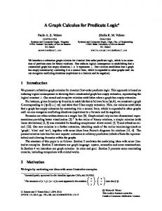
Abstract. Our understanding of basic reasoning with diagrams can be better grasped by observing the following picture: formulas

F1

|=

F2

/

diagrams

_ _

_ _ _ _ _ _ _ _ OO oo DF1 =⇒ DF2 _ _ _ _ _ _ _ _

Based on this picture, we can summarize our work by saying that, in this paper, we show how the basic idea underlying reasoning with diagrams can be nicely adapted to the case of “diagrams” being sets of 2-pointed labeled directed graphs, which define certain binary relations, and “implies” meaning “it is intuitionistically true that relation defined by diagram D1 is a sub-relation of the one defined by diagram D2 , under a set Σ of hypotheses”. We motivate the system, present it formally, prove its soundness, and left the question of its completeness for further investigation. Keywords: Diagrams, Proofs with graphs, Relation algebra, Intuitionistic logic.

1

Introduction

Boolean reasoning, i.e. reasoning involving plain sets and the Boolean operations of union, intersection and complement, may be performed through the algebraic language of Boolean algebras [2]. Likewise, relational reasoning, i.e. reasoning involving relations, the Boolean operations, and the Peircean operations of composition, dual-composition and conversion, may be performed through the more elaborated algebraic language of De Morgan-Peirce-Schröder-Tarski relation algebras [17]. A main difference between these environments arises from the fact

2

R. de Freitas, P. Viana

that, although there is a number of algorithms to decide validity or perform inferences in the calculus with sets [2], the analogous tasks for the relational language are highly undecidable [18]. Hence, the problem of building mechanisms which may help in the design of relational algebraic proofs from scratch arises. The use of mechanized systems to help in the performance of relational inferences is not a new subject of research (cf. [16, 7]). Most of the proposed systems use equational logic [13], that is the high-school rule of replacing equals by equals, as the underlying logic, and thus do not correspond to the predominantly inequational way relational reasoning in naturally performed [14]. Moreover, as can be seen by an examination of some papers where relation algebraic reasoning is developed and applied [4, 15], in practice relation algebraic inferences are performed in an environment consisting of a mixture of equational logic enriched with a sort of lattice theoretical inference engine, i.e the passage from an object to a lesser or from an object to a bigger, at one side of an inclusion. Another drawback of these systems, in our view, is that most of them, with the exception of the systems outlined in [3, 6], make use of the linear format of discourse, in the form of equalities and inclusions between algebraic terms, to represent the information being processed. The authors of this paper, together with some colleagues, have proposed a different mechanism based on diagrams to perform relational reasoning [9, 11, 12]. The environment in which we work can be summarized as follows. As stated earlier, most systems in the bibliography perform inferences with equalities and inclusions between relation algebraic terms. In our work, alternatively, we move to the lattice theoretical side and prefer to handle inclusions rather than equalities, but instead of relation algebraic terms, we use diagrams in the left and right hand sides of an inclusion. We have a set of rules to transform diagrams, in order to test whether an inclusion is a consequence of given a set of inclusions taken as hypotheses. This set of rules work in the following way. Starting with the diagram in the left hand side of the target inclusion, by successive applications of our rules, mediated by the inclusions taken as hypotheses, either we end up with the diagram in the right hand side of the target inclusion, when the inclusion is a consequence of the hypotheses or, otherwise, build a possibly very large non constructive counter model (cf. [12] for details). The main characteristic of the system presented in [12], besides its accordance with reasoning from hypotheses, is an explicit diagrammatic representation of complement, leading to an intuitively simple, playful, and powerful set of rules. The diagrams which represent binary relations may have occurrences of boxed subdiagrams to fit complement, and one of the main transformation rules allows one to change any given diagram into another one, by reproducing it in two parts, one having an occurrence of a subdiagram and the other having an occurrence of the same subdiagram inside a box. This two part diagram represents two complementary alternatives: some relation or its complement holds between some pair of points in the domain. After the use of these diagrams and rules in some concrete situations, one can promptly inquire on the exact strength of the proccess outlined above. In particular, given the resemblance between this

A graph calculus for proving intuitionistic relation algebraic equations

3

proccess and the axiom of the excluded middle of classical first-order logic, one may ask whether is it possible to modify our system in order to obtain a diagrammatic system which can cope with the intuitionistic inferences which can be performed in the relational algebraic language. This is the work we start here. In Section 2, to motivate our work, we present a rough sketch of a problem faced by those who try to build relational equational proofs from scratch: that of finding and justifying the non trivial algebraic laws used in the proof. In Section 3, we summarize, by means of an example, our approach to solve instances of this challenging problem: the use of diagrams. In Section 4, we emphasize that the diagrammatic proofs can be nicely divided in two groups: the classical ones and the intuitionistic ones. Besides, we formalize the previous observation by making a slight change in the set of axioms and rules presented in [12], to produce intuitionistic diagrammatic proofs. In Section 5, we prove the main result of this paper which amounts to the soundness of our diagrammatic rules w.r.t intuitionistic inferences in the relational algebraic language.

2

Algebraic relational proofs

The relation terms, typically denoted by R, S, T , are generated by the following grammar: R ::= r | U | O | I | RC | R−1 | R u R | R t R | R ◦ R, where r belongs to a set of relation variables. A relation inclusion, respectively relation equality, is an expression of the form R v S, respectively R = S. Given a set u, considered as the universe, each relation variable is intended to denote a binary relation on u. Constantes U, O and I denote the universal relation, the empty relation, and the identity relation, respectively. The relation operators C , −1 , t, u, and ◦ denote complementation, conversion, intersection, union and composition, respectively. So, given a set u, the relation terms denote those relations which can be defined from the relations denoted by the variables, by applying the relation operators recursively. Concerning expressive power, the main application of the relation inclusions and equalities is the rewriting of statements involving binary relations, without making any reference to individuals. For example, if r is a binary relation symbol, to express that a relation denoted by r is functional, one may use the first-order sentence ∀xyz(xry∧xrz → y = z) or, equivalently, ∀yz(∃x(xry∧xrz) → y = z). But this can also be expressed throughout a relation inclusion having no occurrences of individual variables. A binary relation r is functional iff it satisfy the inclusion r−1 ◦ r v I. Regarding deductive power, the main application of the relation inclusions and equalities is that using them we can prove certain general facts involving binary relations, applying only equational reasoning or, in most cases, equational reasoning together with a sort of lattice theoretical inference engine. For example, using first-order logic one can easily prove that if two given relations are functional and have disjoint domains, then their union is also a

4


functional relation. But thanks to the fact that x ∈ domr iff ∃y ∈ u(xry) iff ∀z ∈ u(∃y ∈ u(xry ∧ yUz)), statement above can be reformulated in relation algebraic terms as follows. Proposition 1. If r−1 ◦ r v I, s−1 ◦ s v I, and (r ◦ U) u (s ◦ U) = O, then −1 (r t s) ◦ (r t s) v I. A first step to make a relation algebraic proof, in the lattice theoretical style that we are mentioning here, is to find out some algebraic laws to help you in the development of the proof. In the case of Proposition 1, the use of some obvious −1 laws such as (r t s) = r−1 t s−1 is easy to predict, while the correct way to choose and apply the more elaborated ones just come after some ingenuity allied to experience in trying to produce these proofs. As an example, a useful law for this case states that the following equivalences hold for any relations r, s, t: r ◦ s v t ⇐⇒ r−1 ◦ tC v sC ⇐⇒ tC ◦ s−1 v rC .

(1)

From (1), the proof of Proposition 1 breaks down in three main steps. First, we prove r−1 ◦ s = O, from the hypothesis (r ◦ U) u (s ◦ U) = O, as follows: (r ◦ U) u (s ◦ U) = O ⇐⇒ r ◦ U v (s ◦ U) ⇐⇒ ⇐⇒ ⇐⇒ ⇐⇒

C

CC

r−1 ◦ (s ◦ U) v UC r−1 ◦ (s ◦ U) v O (r−1 ◦ s) ◦ U = O r−1 ◦ s = O.

Second, from this, we obtain s−1 ◦ r = O. Finally, we complete the proof: (r t s)

−1

◦ (r t s) = (r−1 t s−1 ) ◦ (r t s) = (r−1 ◦ r) t (r−1 ◦ s) t (s−1 ◦ r) t (s−1 ◦ s) vItOtOtI = I.

Of course, the outlined proof can only be considered as a proof if all details left to the reader are filled and all general laws applied are either justified from a set of axioms or taken as axioms themselves. This is an easy task for certain laws and equivalences such as r ◦ (s ◦ t) = (r ◦ s) ◦ t or r u s = O ⇐⇒ r v sC , but someone may be uncomfortable with our use of (1) and may ask for a justification.

3

Diagrammatic relational proofs

With the previous example, we want to emphasize that the (far from being deterministic) main step in producing a relation algebraic proof of an inclusion or equality from a set of inclusions or equalities taken as hypotheses, consists in the choice of a nice set of relation algebraic laws to assist you in building the proof.


5

The finding of these laws may be guided by experience, previous knowledge, luck, etc, but, whatever the medium used to find them, the laws used in the proof must ultimately be justified. The authors of this paper, together with some colleagues, have been trying a strategy based on diagrams. To exemplify our approach, let us explain how some sort of graphs can be used to produce a very convincing proof of Proposition 1, and even of the capital law (1). The main idea of our approach in proving a relation inclusion R v S from a set of hyphoteses is to associate diagrams DR and DS to the left and the right hand sides of the inclusion and, by the application of the hypotheses according certain rules, to transform diagram DR into diagram DS . In this case, certainly due to the conceptual proximity between binary relations and graphs, the diagrams that appear as the most appropriate to deal with are sets of 2-pointed labeled directed graphs [1, 5], which we simply call diagrams. Besides, a complete set of rules is given by considering the tranformation rules in [12]. We describe the most important ones in very general terms in Table 1. Table 1. Informal explanation of some transformation rules. Cv

Any subdiagram D1 of a diagram D can be replaced by another diagram D2 that contains the information given by D1 , and possibly less information. Hyp Given a diagram D and an inclusion R v S, any subdiagram of D containing the information given by DR can be replaced by another subdiagram that contains the information given by DS . Hyp∗ Any diagram D can be broken into another one, let us say D1 |D2 , containing two alternatives: D1 contains the information given by D in conjunction with a piece of information i, and D2 contains the information given by D in conjunction with the information complementary to i. Hyp∅ Any subdiagram containing contradictory information can be erased.

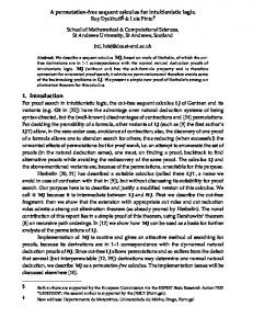
This set of rules plus other very intuitive ones used to iteratively transform relation terms in diagrams (cf. [12]), allow us to drawn Figure 1, containing a diagrammatic proof of Proposition 1. The proof consists of a sequence (D1 , D2 , D3 , D4 , D5 , D6 , D7 , D8 ) of eight diagrams. D1 is an arc labeled with −1 the term (r t s) ◦ (r t s). This is just the diagram associated to the term, representing the left hand side of the inclusion we want to proof. D2 is obtained −1 from the D1 by replacing the arc labelled with the term (r t s) ◦ (r t s), having one main occurrence of composition, by two consecutive arcs, one labelled −1 (r t s) and the other labeled r t s. D3 is obtained from D2 by replacing the −1 arc labelled with the term (r t s) , having one main occurrence of conversion, by one arc labelled r t s which has the opposite direction to the arc it replaced. Now, the left arc in D3 , labelled r t s, represents two alternatives, one is r and the other is s. So, D4 is obtained from D3 by replacing it with a diagram consisting of two similar subdiagrams, one with the left arc labelled r, representing the first alternative, and the other with the left arc labeled s, representing the second alternative. In a entirely similar way, we obtain D5 from D4 , by considering the alternatives given by the labels r t s with occur in the right arc of

6


both subdiagrams. Now, we have D5 , a diagram consisting of four alternatives, each one represented by a subdiagram. Observe that according to the hyphotesis r−1 ◦ r v I, the first alternative presented in D5 is included in I. Then we have diagram D6 . Analogously, using the hypothesis s−1 ◦ s v I, we obtain D7 . Moreover, according to the hyphotesis (r ◦ U) u (s ◦ U) = O the second and third alternatives in D7 are inconsistent. So, they should be simply erased. Finally, we end up with D8 , consisting of an arc labelled I. That is the diagram of the right hand side of the inclusion we want to prove. (rts)T ◦ (rts)

−

D1 :

/+

m Comp −

D2 :

(rts)T

/•

rts

/+

m Rev −o

D3 :

rts

•

rts

/+

m Uni −o

D4 :

r

•

rts

−o

/+

s

•

/+

rts

m Uni; Uni

D5 :

−o

r

•

r

−o

/+

r

•

s

−o

/+

s

•

r

/+

−o

s

•

r

/+

r

/+

−o

s

•

s

/+

⇓ HyprT ◦rvI −

D6 :

I

−o

/+

r

•

s

−o

/+

s

•

⇓ HypsT ◦svI

D7 :

−

I

/+

−o

r

•

s

/+

−o

s

•

r

/+

⇓ Hyp(rts)T ◦ (rts)vO D8 :

−

I

/+

Fig. 1. Diagramatic proof of Proposition 1.

Now, as we mentioned, the capital law used in the relation algebraic proof of Proposition 1, given above, was (1). Someone unconfortable with it may wish to


7

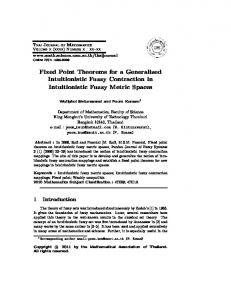
use our transformation rules to produce a convincing proof of it. We present, in Figure 3,a diagrammatic proofjustifying the implication r ◦ s v t =⇒ r−1 ◦ tC v sC . It consists of a sequence (D1 , D2 , D3 , D4 , D5 , D6 , D7 , D8 ) of eight diagrams. D1 is the diagram representing the term r−1 ◦ tC , i.e D1 represents the left-hand side of the inclusion we want to prove. D2 is obtained from D1 by replacing the main occurrence of composition by two consecutive arcs, labeled r and tC , respectively. D3 is obtained from D2 by replacing the arc r−1 by an arc labeled r in the opposite direction, and the arc tC , labelled with a term having one main t

occurrence of complementation, by one arc labelled − → + . We agree that a box around a diagram represent the negation of the information represented by that diagram. Now, D4 is obtaneid from D3 by replacing it by a diagram consisting of two subdiagrams representing two alternatives. We agree that, in general, a diagram represents alternatives a pair of points may satisfy in order to belong to the relation represented by the diagram. Also, as usual, any pair of points is related by a given relation or by its complement. Thus, by displaying two complementary alternatives to the same pair of nodes, diagram D4 impose the same restrictions to any pair of nodes that is imposed by diagram D3 , i.e both D3 and D4 represent the same relation. D5 is obtained from D4 , according to the following idea that allow us to use the hypothesis r ◦ s v t to transform diagram D4 . Since the left subdiagram of D4 has a path from − to + through • that represents the relation r◦s and since, by hypothesis, r◦s v t, we are allowed to transform D4 by adding an arc labeled t from − to +. Now, observe that the left subdiagram of D5 has two parallel arcs linking node • to +, one labeled t t

and the other labeled − → + . We agree that parallel paths linking the same points mean that the points are simultaneously in the relations represented by each path. So, nodes • and + are simultaneouly in relations t and tC , so that the left subdiagram of D5 represents inconsistent information. Thus, we can erase it from D5 , obtaining D6 . Now, note that, inside D6 we can locate a copy of the diagram represeting s , as shown in Figure 2.

−

t

/+

/7 + m ooo o o o s ooo /+ − oooo m

• r

−

−

o7 + ooo o o o ooo s /+ ooo −

Fig. 2. Mapping diagram representing sC into D6 .

This means that D7 imposes no more restrictions than D6 in defining a relation and so, D6 may be considered to represent a sub-relation of D7 . Thus, we finally move from diagram D7 to diagram D8 , that represents the right-hand side of the implication we want to prove.

8


/+

r T ◦tC

−

D1 :

m Comp −

D2 :

/•

rT

tC

/+

m Rev; Neg −o

D3 :

D4 :

/+

• Hyp∗

⇓

/+ /5 + • kkkk k k r k kkkk s − −

/+

t

−

r

t

−

t

/+

k/5 + kkkk k k k kkk s /+ − − •

r

∗

⇓ Hypr◦svt −

D5 :

t

/+

−

/ • 5/ + t kkkk k r kkkkkks −

t

/+

/5 + kkkk k k k kkkk s / − − + •

r

∗

Hyp∅

⇓ −

/+

t

/+ kkk5 k k k kkkkk s / − − + •

D6 :

r

⇓ Cv − D7 :

s

/+

−

/+

m Neg D8 :

−

sC

/+

Fig. 3. Diagrammatic proof of r ◦ s v t ì r−1 ◦ tC v sC .


9

We think that diagrammatic reasoning should talk by itself. So, we hope the explanations above are sufficient to give the reader a good idea of how our system works. The attentive reader may have noticed the unexplained use we made of the symbol ∗ in the proofpresented in Figure 3. There, this tag was introduced whenwe applied the rule that allows us to transform a diagram by breaking it in two parts, each one containing alternative complementary information. This passage occurred when we transformed diagram D2 into diagram D3 . The tag was used to label the subdiagram which does not have the occurrence of the negated information, expressed in the form of a boxed term or diagram, and continued until the end of the proof, or, as in the case of this proof, until some derived information containing the tag was erased by the application of the appropriated rule. Hence, the diagrammatic proofs presented in Section 3 are of two kinds: those whose last diagram has occurrences of the tag ∗ and those whose last diagram does not have occurrences of ∗. By experimenting with this idea, we observed that the proofs ending with diagrams without occurrences of tag correspond to intuitionistic inferences and those ending in diagrams having occurrences of tag correspond to non intuitionistic ones. Hence, we decided to explore this characteristic of our calculus, adapting it to prove all the intuitionistic inferences expressible in its language. To this, we introduced the tag formally and we made all the necessary amendments to obtain an adequated intuitionistic diagrammatic system. In the next sections, we present these ideas formally and proof soundness of a calculus with graphs for the intuitionistic logic of binary relations.

4

Intuitionisitc graph calculus

Nodes and labeled arcs are the building blocks of graphs. Hence, we first consider the sets Inod of individual nodes and Rvar of relation variables, which we will keep fixed throughout. A graph, typically denoted by G or H, is a structure (N, A, i, o, t), where N is a finite nonempty set of nodes, A ⊆ N × L × N is a finite set of labeled arcs (L is the set of all labels), i (input) and o (output) are, not necessarily distinct, distinguished nodes in N , and t is a finite sequence of natural numbers (tag). An arc of A is a triple, denoted by uLv, with u, v ∈ N and L being a label. A label is a relational symbol or a box D , where D is a concrete diagram. A concrete diagram is a set of graphs. Graphs G1 = (N1 , A1 , i1 , o1 , t1 ) and G2 = (N2 , A2 , i2 , o2 , t2 ) are isomorphic if there are bijections f : N1 → N2 and g : A1 → A2 such that (1) for all urv ∈ A1 , g(urv) = f urf v; (2) for all u D v ∈ A1 , g(u D v) = f u D0 f v and D and D0 are isomorphic; and (3) f i1 = i2 and f o1 = o2 . Concrete diagrams D and D0 are isomorphic if there is a bijection h : D → D0 such that h(G) is isomorphic to G, for all G ∈ D. The usual identification of isomorphic concrete diagrams is reflected in our figures by the representation of every non-distinguished node by •, of every input node by −, and of every

10


output node by +. In figures, tag h1i is represented by ∗. A diagram is an equivalence class of isomorphic concrete diagrams. In what follows, a diagram is identified with each of the concrete diagrams that represents the equivalence class. A diagram inclusion is an expression of the form D v D0 . Now we present a set of axioms and a set of rules to transform a diagram into another. We first introduce two families of axioms of our graph calculus. Given a graph G = (NG , AG , iG , oG , tG ), we define two diagrams as follows. The graph OG := {(NG , AG ∪ {iG {G} oG }, iG , oG , tG )} is obtained from G by adding to it a new arc from the input of G to the output of G labeled by {G} . The graph EG := {(NG , AG , iG , oG , h1i), ({i, o}, {i {G} o}, i, o, h i)} is obtained from G by adjoining to G a new slice with two distinct nodes, input i and output o, and a single arc i {G} o. We shall take as schemes of axioms of the graph calculus the inclusions OG v O and E v EG for any graph G (Table 2). The rules of our graph calculus are the Introduction/Elimination rules (one for each operator), Graph Cover rule, Hypotheses rule and Box rule. Introduction/Elimination rules covers the labels of the graphs. Graph Cover rule is used to compare diagrams with respect to inclusion, Hypotheses rule, to transform diagrams according to the set of inclusions taken as hypotheses, and Box rule, to simplify the inner structure of box labels. Introduction/Elimination rules are presented in Table 2. Each one of these rules can be applied in both directions: downward and upward, allowing the elimination (downwards) and the introduction (upwards) of the operators. We will explain each two-way rule in the downward direction. Each one of these rules involves the application of the local transformation specified in the rule, leaving the rest of diagram untouched. Introduction/Elimination rules, except for Imp, are similar to those of the graph calculus presented in [10] and their presentation are taken from this paper. Rule Univ allows erasing an arc labeled by U from a graph. Rule Vd allows erasing a graph having an arc uOv. Rule Iden allows erasing an arc uIv and a node u, renaming nodes and redirecting arcs accordingly. We use the node substitution notation uv for replacing u by v, which we extend naturally to sets as well as to tuples, e.g., for a set A of arcs, we put A uv = {w uv Lz uv : wLz ∈ A}. Given a relation term R, the diagram associated to R is DR ::= ({i, o}, {iRo}, i, o, h i). Rule Neg allows replacing an arc uRC v by an arc u DR v. Rule Rev allows replacing an arc uR−1 v by vRu. Rule Int allows replacing an arc uR u Sv by arcs uRv and uSv. Rule Uni allows replacing a graph G having an arc uR t Sv by


11

two other graphs GR and GS , obtained from G by replacing the arc uR t Sv by new arcs uRv and uSv, respectively. Rule Imp allows replacing a graph G having an arc uR A Sv by two other graphs G∗R and GS , obtained from G by replacing the arc uR A Sv by new arcs u DR v and uSv, respectively, and by adding the lower natural number not occurring in any tag in the graph proof to the tag of G∗R . Rule Comp allows replacing an arc uR ◦ Sv by arcs uRw and wSv, with a new node w. To define our next transformation rule, the concepts of homomorphism from a graph to another and that of a diagram covering another will be crucial. Given graphs G = (NG , AG , iG , oG , tG ) and H = (NH , AH , iH , oH , tH ), by a graph homomorphism from H to G we mean a function φ : NH → NG , denoted by φ : H → G, that preserves input, output, and arcs, i.e. φiH = iG , φoH = oG , and if uLv ∈ AH then φuLφv ∈ AG . Given diagrams D1 and D2 , we say that D2 covers D1 or D1 is covered by D2 , denoted by D1 ← D2 , iff for each graph G ∈ D1 there exist a graph H ∈ D2 and a graph homomorphism φ : H → G. To define our next transformation rule, the concepts of homomorphism from a graph to another and that of a diagram covering another will be crucial. Given graphs G = (NG , AG , iG , oG , tG ) and H = (NH , AH , iH , oH , tH ), by a graph homomorphism from H to G we mean a function φ : NH → NG , denoted by φ : H → G, that preserves input, output, and arcs, i.e. φiH = iG , φoH = oG , and if uLv ∈ AH then φuLφv ∈ AG . Given diagrams D1 and D2 , we say that D2 covers D1 or D1 is covered by D2 , denoted by D1 ← D2 , iff for each graph G ∈ D1 there exist a graph H ∈ D2 and a graph homomorphism φ : H → G. Rule Cv (Table 2) allows replacing a diagram by another one that covers it. We now introduce the concepts of gluing graphs and draft homomorphism between graphs, which will be central in applying a diagram inclusion to transform a diagram into another. Intuitively, we glue graph H onto graph G by adding to G a copy of H and identifying designated nodes u, v of G to the input and output of H. More precisely, given graphs G = (NG , AG , iG , oG , tG ) and H = (NH , AH , iH , oH , tH ), as well as designated nodes u, v ∈ NG , the result of gluing H onto G via u, v is the graph defined by glue (u,v)k (H, G) := (NG ] NH , AG ] AH , iG , oG , tG ktH ) iuH ovH , where k is a given function associating tags to tags. We glue a diagram D onto a graph G, via nodes u, v of G, by gluing its graphs to G, i.e. glue (u,v)k (D, G) := {glue (u,v)k (H, G) : H ∈ D}. Given graphs G = (N, A, i, o, t) and G0 = (N 0 , A0 , i0 , o0 , t0 ), by a draft homomorphism from G0 to G we mean a function θ : N 0 → N , denoted by θ : G0 99K G, that preserves arcs. Now, given graphs G and G0 as before, a draft homomorphism θ : G0 99K G, and diagram D, we set glue θk (D, G) := glue (θi0 ,θo0 )k (D, G). Rule HypΓ (Table 2) allows gluing a diagram D onto a graph G of a diagram under a draft homomorphism θ : G0 99K G when D0 ∪ {G0 } v D is a hypothesis in Γ or is an axiom. The Box rule (Table 2) is a two-way rule, i.e. it can be applied in the topdown and in the bottom-up directions. In the top-down direction, the Box rule allows replacing an arc labeled by a box D having a diagram D = {Gj : j ∈ J}

12


Table 2. Axioms and rules for transforming diagrams. Axioms OG v O

E v EG

and

Elimination/Introduction rules Univ

Iden

(N, A ∪ {uUv}, i, o, t) (N, A, i, o, t)

G ∪ {(N, A ∪ {uIv}, i, o, t)} G ∪ {(N, A, i, o, t) uv }

Rev

(N, A ∪ {uR−1 v}, i, o, t) (N, A ∪ {vRu}, i, o, t) Uni

Imp

Vd

D ∪ {(N, A ∪ {uOv}, i, o, t)} D (N, A ∪ {uRC v}, i, o, t)

Neg

(N, A ∪ {u DR u}, i, o, t) Int

(N, A ∪ {uR u Sv}, i, o, t) (N, A ∪ {uRv, uSv}, i, o, t)

D ∪ {(N, A ∪ {uR t Sv}, i, o, t)}) D ∪ {(N, A ∪ {uRv}, i, o, t), (N, A ∪ {uSv}, i, o, t)} D ∪ {(N, A ∪ {uR A Sv}, i, o, t)}

if n is the D ∪ {(N, A ∪ {u DR v}, i, o, tn), (N, A ∪ {uSv}, i, o, t)} lower natural number not occurring in any tag in the graph proof Comp

(N, A ∪ {uR ◦ Sv}, i, o, t) (N ∪ {w}, A ∪ {uRw, wSv}, i, o, t)

if w 6∈ N

Graph Cover rule Cv

D1 D2

if D1 ← D2

Hypotheses rule HypΓ

D1 ∪ {G} D1 ∪ glue θk (D2 , G)

tn if t 6= h i t otherwise where n is the lower natural number not occurring in any tag in the graph proof if θ : G0 99KG and D0 ∪ {G0 } v D2 is in Γ or is an axiom, and kt =

Box rule D ∪ {(N, A ∪ {u {Gj : j ∈ J} v}, i, o, t)} Box D ∪ {(N, A ∪ {u {Gj } v : j ∈ J}, i, o, t)}


13

inside of it, by a set of parallel arcs, each one labeled by a box {Gj } , and vice-versa, for the bottom-up direction. In the case I = ∅, the Box rule allows erasing (top-down) or to add (bottom-up) an arc labeled by a box with the empty diagram O inside of it. The notion of derivation is standard. Given a set of diagram inclusions Γ , by a derivation from Γ , or simply a Γ -derivation, we mean a sequence (D0 , . . . , Dn ) of diagrams such that each diagram Dk , for k ∈ {1, . . . , n}, is obtained from diagram Dk−1 by an application of one of the inference rules (Introduction/Elimination, Cv, HypΓ , or Box). A diagram D0 is derivable from a diagram D using Γ , or simply D0 is Γ -derivable from D, denoted by Γ ` D v D0 , when there is a Γ -derivation (D0 , . . . , Dn ) such that D0 = D and Dn = D0 . An inclusion D v D0 is a theorem, denoted by ` D v D0 , when D0 is derivable from D using the empty set of hypotheses. A diagram D0 is intuitionistic derivable from a diagram D using Γ , or simply 0 D is Γ -i-derivable from D, denoted by Γ ì D v D0 , when there is a Γ derivation (D0 , . . . , Dn ) such that D0 = D, Dn = D0 , and all natural numbers occurring in the tags of graphs of D0 also occur in tags of graphs of D or of some diagram of the inclusions in Γ . An inclusion D v D0 is an intuitionistic theorem, denoted by ì D v D0 , when D0 is i-derivable from D using the empty set of hypotheses.

5

Soundness of the calculus

Let R be a relational term and u, v be individual variables. The uv-translation of R into a first-order formula is defined recursively as follows: STuv(r) = r(u, v), if r is a relational variable; STuv(U) = >; STuv(O) = ⊥; STuv(RC ) = ¬STuv(R); STuv(R−1 ) = STvu(R); STuv(R u S) = STuv(R) ∧ STuv(S); STuv(R t S) = STuv(R) ∨ STuv(S); and STuv(R ◦ S) = ∃w(STuw(R) ∧ STwv(S)), with w being a new variable. The standart translation of R is STxy(R). We define the standard translation of diagrams into first-order formulas in such a way that ST(DR ) = ST(R). Let us consider the set Inod of all nodes as a set of individual variables. Assume that x, y 6∈ Inod. The standard translation of an arc a into a first-order formula is ST(a) = STuv(R), if a = uRv, and ST(a) = ¬ST(D) ux yv , if a = u D v. The standard translation of V a graph G = (N, A, i, o, t) into a first-order formula is ST(G) = ∃N \ {i, o} a∈A ST(a) xi yo . Remember that x, y 6∈ N , for every graph G = (N, A, i, o, t). The standard translation of a diagram D = {G1 , . . . , Gn } into a first-order formula is ST(D) = ST(G1 )∨· · ·∨ST(Gn ). It is immediate from these definitions that ST(DR ) = ST(R). Theorem 1. Let Γ ∪ {D v D0 } be a finite set of diagram inclusions. If Γ ì D v D0 and every natural number in the tag of every graph in D0 also occurs in a tag of a graph in D or in Γ , then ST(D0 ) is an intuitionistic consequence of ST(D) and ST(Γ ).

14


Proof. Let (D0 , . . . , Dn ) be a Γ -i-derivation of D0 from D. We prove by induction on n that ST(Dn ) is an intuitionistic consequence of ST(D) and ST(Γ ). If D0 is Γ -i-derivable from D by only one application of some rule, then this rule is neither HypEvEH nor Imp, since both of them add a new natural number in a tag of a graph. Moreover, we have the following fact, that can be stablished by a tedious examination of cases. Fact 1. If Di derived from Di−1 by an application of any inference rule, except HypEvEH and Imp, using Γ , then ST(Di ) is an intuitionistic consequence of ST(Di−1 ) and ST(Γ ), where ST(Γ ) = {ST(γ) : γ ∈ Γ }. Hence, if n = 1, then ST(D0 ) is an intuitionistic consequence of ST(D) and ST(Γ ). Now, let (D0 , . . . , Dk+1 ) be a Γ -i-derivation of D0 from D. As (D1 , . . . , Dk+1 ) is a Γ -i-derivation of D0 from D1 of lenght k, by the IH, ST(Dk+1 ) is an intuitionistic consequence of ST(D1 ) and ST(Γ ). We consider two cases. Case 1. D1 is derived from D0 by an application of any inference rule, except HypEvEG and Imp, using Γ . In this case, by Fact 1, ST(D1 ) is an intuitionistic consequence of ST(D0 ) and ST(Γ ). Hence, ST(Dk+1 ) is an intuitionistic consequence of ST(D0 ) and ST(Γ ), i.e., ST(D0 ) is an intuitionistic consequence of ST(D) and ST(Γ ). Case 2. D1 is derived from D0 by either an application of HypEvEH or of Imp. In this case, D0 = Dhi ∪ {G} and D1 = Dhi ∪ {Ghi , Gm }, where — {Ghi , Gm } = glue θk (EH , G), Gm is a graph with a new natural number m in its tag and Ghi is a graph with the same tag as G, if the applied rule is HypEvEH ; — G = (N, A ∪ {uR A Sv}, i, o, t), Ghi = (N, A ∪ {uSv}, i, o, t), Gm = (N, A ∪ {u DR v}, i, o, tm), and m is a new natural number. If the applied rule is HypEvEH , or if it is Imp, we have the following results. Fact 2. Γ ì {Gm } v ∅ — Since m does not occur in D0 and the only way to delete a tag is to apply rule Vd. Then, by the IH, ST(∅) = ⊥ is an intuitionistic consequence of ST(Gm ) and ST(Γ ), since the Γ -i-derivation of ∅ from Gm is contained in (D1 , . . . , Dk+1 ). We say that a Γ -derivation (D1 , . . . , Dn ) is contained in a Γ -derivation δ if D1 ⊆ D10 , . . . , Dn ⊆ Dn0 for some subsequence (D10 , . . . , Dn0 ) of δ. Hence, since {Ghi , Gm } = glue θ (EH , G): ST(Dhi∪ {Ghi}) is an intuitionistic consequence of ST(Dhi∪ {G}) and ST(Γ ) (2) Fact 3. Γ ì Dhi ∪ {Ghi } v D0 — By the I.H., ST(D0 ) is an intuitionistic consequence of ST(D1 ) and ST(Γ ). Recall that D1 = Dhi ∪ {Ghi , Gm }. Then, since m occurs in Gm but not in D0 , we have Γ ì Dhi ∪ {Ghi , Gm } ì D0 . Hence, by the IH, since the Γ -i-derivation of D0 from Dhi ∪{Ghi } is contained in (D1 , . . . , Dk+1 ): ST(D0 ) is an intuitionistic consequence of ST(Dhi ∪{Ghi }) and ST(Γ )

(3)

From (2) and (3), ST(D0 ) is an intuitionistic consequence of ST(D0 ) and ST(Γ ), since D0 = Dhi ∪ {G}. Hence, ST(D0 ) is an intuitionistic consequence of ST(D) and ST(Γ ).


15

Corollary 1. Let Γ = {Rj v Sj : j ∈ J} ∪ {R v S} be a finite set of inclusions. Hence, if {DRj v DSj : j ∈ J} ì DR v DS , then ∀xy(ST(R) → ST(S)) is an intuitionistic consequence of {∀xy(ST(Rj ) → ST(Sj )) : j ∈ J}. Proof. Immediate from Theorem 1, since for any relation term R, we have ST(DR ) = ST(R). By the definition of DR and the fact that, if ST(D0 ) is an intuitionistic consequence of ST(D) and ST(Γ ), then ∀x∀y(ST(D) → ST(D0 )) is an intuitionistic consequence of ST(Γ ), since the only free variables of ST(D) and ST(D0 ) are x and y, and formulas in ST(Γ ) have no free variables.

References 1. H. Andréka, D.A. Bredikhin. The equational theory of union-free algebras of relations. Algebra Universalis 33:516–532, 1995. 2. F.M Brown. Boolean reasoning: the logic of Boolean equations. Dover, 2003. 3. D. Cantone, A. Formisano, E. G. Omodeo, C. G. Zarba. Compiling dyadic specifications into map algebra. Theoret. Comput. Sci. 293: 447–475, 2003. 4. L.H. Chin, A. Tarski. Distributive and modular laws in the arithmetic of relation algebras. University of California Publications in Mathematics – New Series 1: 341–384, 1951. 5. S. Curtis, G. Lowe. Proofs with graphs. Sci. Comput. Programming 26:197–216, 1996. 6. A. Formisano, E. G. Omodeo, M. Simeoni. A graphical approach to relational reasoning, ENTCS 44: 1–22, 2003. 7. S. Foster, G. Struth, T. Weber. Automated engineering of relational and algebraic methods in Isabelle/HOL. LNCS 6663:52-67, 2011. 8. R. de Freitas, P. Viana. A note on proofs with graphs. Sci. Comput. Programming 73:129-135, 2008. 9. R. de Freitas, P. A. S. Veloso, S. R. M. Veloso, P. Viana. On positive relational calculi. Logic J. IGPL 15: 577–601, 2007. 10. R. de Freitas, P. A. S. Veloso, S. R. M. Veloso, P. Viana. On a graph calculus for algebras of relations. LNCS 5110: 298–312, 2008. 11. R. de Freitas, P. A. S. Veloso, S. R. M. Veloso, P. Viana. On graph reasoning. Inform. and Comput. 207:1000-1014, 2009. 12. R. de Freitas, P. A. S. Veloso, S. R. M. Veloso, P. Viana. A calculus for graphs with complement. LNAI 6170: 84–89, 2010 . 13. L. Henkin. The logic of equality. Amer. Math. Monthly 84: 597–612, 1977. 14. P. H¨ ofner, G. Struth. On automating the calculus of relations. LNCS 5195: 50–66, 2008. 15. Y. Kawahara. Applications of relational calculus to computer mathematics. Bulletin of informatics and cybernetics, 23: 67–78, 1988. 16. D. von Oheimb, T.F. Gritzner. RALL: Machine-supported proofs for relation algebra. LNCS 1249:380-394, 1997. 17. G. Schmidt, T. Str¨ ohlein. Relation and Graphs: discrete mathematics for computer scientists. Springer, Berlin, 1993. 18. A. Tarski, S. Givant. A Formalization of Set Theory Without Variables. American Mathematical Society, 1987.