A Port Graph Calculus for Autonomic Computing and Invariant ...

Author manuscript, published in "TERMGRAPH 2009, 5th International Workshop on Computing with Terms and Graphs, Satellite Event of ETAPS 2009, York : United Kingdom (2009)"

Replace this file with prentcsmacro.sty for your meeting, or with entcsmacro.sty for your meeting. Both can be found at the ENTCS Macro Home Page.

A Port Graph Calculus for Autonomic Computing and Invariant Verification Oana Andrei1 inria-00418560, version 1 - 20 Sep 2009

Department of Computing Science, University of Glasgow, Glasgow G12 8RZ, UK

H´el`ene Kirchner2 INRIA Bordeaux Sud-Ouest, 351, Cours de la Lib´ eration, F-33405 Talence, France

Abstract From our previous work on biochemical applications, the structure of port graph (or multigraph with ports) and a rewriting calculus have proved to be well-suited formalisms for modeling interactions between proteins. Then port graphs have been proposed as a formal model for distributed resources and grid infrastructures, where each resource is modeled by a node with ports. The lack of global information and the autonomous and distributed behavior of components are modeled by a multiset of port graphs and rewrite rules which are applied locally, concurrently, and non-deterministically. Some computations take place wherever it is possible and in parallel, while others may be controlled by strategies. In this paper, we first introduce port graphs as graphs with multiple edges and loops, with nodes having explicit connection points, called ports, and edges attaching to ports of nodes. We then define an abstract biochemical calculus that instantiates to a rewrite calculus on these graphs. Rules and strategies are themselves port graphs, i.e. first-class objects of the calculus. As a consequence, they can be rewritten as well, and rules can create new rules, providing a way of modeling adaptive systems. This approach also provides a formal framework to reason about computations and to verify useful properties. We show how structural properties of a modeled system can be expressed as strategies and checked for satisfiability at each step of the computation. This provides a way to ensure invariant properties of a system. This work is a contribution to the formal specification and verification of adaptive systems and to theoretical foundations of autonomic computing. Keywords: Port graph, port graph rewriting, rewriting calculus, biochemical calculus, rewriting strategies, adaptive systems, autonomic computing, invariant verification.

1

Introduction

Autonomic computing refers to self-manageable systems initially provided with some high-level instructions from administrators. It gained much interest with the recent development of large scale distributed systems such as service infrastructures and grids. For such adaptive systems, there is crucial need for theories and formal frameworks to model computations, to define languages for programming and to establish foundations for verifying important properties of these systems. 1 2

Email: [email protected] Email: [email protected] c 2009

Published by Elsevier Science B. V.

inria-00418560, version 1 - 20 Sep 2009

Andrei and Kirchner

In [3] we have introduced the structure of port graph, port graph rewrite rules and a rewriting relation for port graphs. We have designed this formalism for modeling complex systems with dynamical topology whose components interact in a concurrent and distributed manner. Nodes with ports represent components (or objects), while edges correspond to communication channels. Then port graph rewrite rules are used for modeling the interactions between some entities or nodes, capable of creating connections among them at specific points (ports), breaking connections, merging, splitting, or deleting nodes, or performing any combination of these operations. A dynamic system whose initial state is represented by a port graph structure evolves according to a set of port graph rewrite rules leading to changes in its structure over time. We have defined a higher-order formalism, the ρpg -calculus, where the system state and the system behavior are described at the same level. More expressive power is gained in modeling a system evolution via port graph rewrite rules that may introduce other port graph rewrite rules and via strategies for controlling the application of a set of port graph rewrite rules. We have already shown the capabilities of the ρpg -calculus to model adaptive systems and biochemical networks [1,4]. Once a formal specification framework for such systems has been set up, the next step that comes naturally is to provide an automated method for validating the behavior of the system with respect to some initial design requirements or properties. A main contribution of this paper is the enrichment of the calculus with a method for verifying a given set of structural properties for a modeled system. We express the requirements that a system behavior has to meet as structural formulas using a suitable syntax and we embed them at the same level as the system description. Then the structure of the modeled system is dynamically verified to satisfy the given requirements. We encode the structural formulas by means of adequate rewrite strategies and we verify that the modeled system satisfies them using the evaluation mechanism of rewrite strategies. We obtain a kind of runtime verification technique which allows the running system to detect its own structural failures. Usually, this verification technique increases the confidence in the correctness of the system behavior with respect to its formal specification. In particular, for adaptive systems, runtime verification is useful for recovering from problematic situations, hence for ensuring a self-healing property. The paper is structured as follows. Section 2 defines the notions of port graphs, port graph rewrite rules and port graph rewriting, illustrating them by molecular graph rewriting in a biological model. Then Section 3 presents an abstract rewriting calculus inspired by biochemical transformations in which molecules are collections of structured objects, rules and more general abstractions. An interaction taking place between an abstraction and a molecule is a step of the calculus. Introducing application and failure allows the definition of more general forms of abstractions called strategies to express control on rule application in the same formalism. Section 4 extends the formal framework to verify structural properties of systems. We show how properties of a modeled system can be expressed as strategies and checked for satisfiability at each step of the computation. This provides a way to ensure invariant properties of a system. Further research perspectives are given in the conclusion. All proofs of the results presented in this paper can be found in [1]. 2

Andrei and Kirchner

2

Port Graphs and Port Graph Rewriting

Port graphs are a particular class of graphs, where nodes have explicit connection points called ports with the edges attached to specific ports of nodes. This graph structure is inspired by the molecular complexes formed in protein-protein interactions in a biochemical network: a protein is characterized by a collection of small patches on its surface, called functional domains or sites, and two proteins can bind on such sites. Then a protein with its collection of sites is modeled by a node with ports, and a bond between two proteins by an edge in a port graph.


Example 2.1 Let us consider a fragment of the epidermal growth factor receptor (EGFR) signaling pathway, an example often studied in the context of various formalisms, the κ-calculus [16,19] for instance. The species in this model are: •

the signal protein EGF situated outside the cell acting as a ligand,

•

the transmembrane protein EGFR with two extracellular sites and two intracellular sites as a receptor, and

•

the adapter protein SHC situated inside the cell.

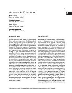
The behavior of a protein is given by its functional domains that determine which other protein it can bind to or interact with. These domains are usually abstracted as sites that can be bound or free, visible or hidden. A protein is characterized by the collection of interaction sites on its surface. Proteins can connect at specific sites by low energy bounds forming molecular complexes. A biochemical system is represented as a discrete system consisting of interacting components which gives rise to structural and behavioral transformation of the components and of the system as a whole. Such a system is dynamic, has an emergent behavior, is highly concurrent and non-deterministic. We represent a protein as an empty box having the identifier placed at the exterior and the sites as small points on the surface of the box. For proteins the ports are called sites and the edges bonds. Graphically, the state of a site is represented as a filled circle for bound, an empty circle for free, and a slashed circle for hidden. Then the three types of proteins above are represented graphically as in Figure 1. 2

1

EGF

3

2 4

1

EGFR

2

1

SHC

Fig. 1. The species in the EGFR signaling pathway fragment

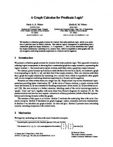
In the left side of Figure 2 we illustrate an initial state of the system modeling the signaling pathway and on the right, an intermediary state where two signal proteins are already bound forming a dimer which in turn is bound to a receptor. Before giving the formal definition of port graphs [1,4], let us start by defining the way ports are associated to node names via a signature. Definition 2.2 [P-Signature] A p-signature is a pair of sets of names ∇ = h∇N , ∇P i where ∇N is a set of node names and ∇P is a set of port names such that each node name N comes with a finite set of ports Interface(N ) ⊆ ∇P . 3

Andrei and Kirchner

1:EGF 2

1

5:EGFR

2:EGF 2

3

3:EGF 2

1

2 4

1

2

1

3

7:SHC

1.2:EGF.EGF

4:EGF

2 4

1

2

1 1

1

5:EGFR

6:EGFR

1

2

3

3.4:EGF.EGF

2

2

2 4

1

3

7:SHC

G

2 4

1 1

2

1

2

6:EGFR

1

G'

Fig. 2. Initial and intermediate port graphs in the EGFR model


The port names associated to a node name are assumed to be pairwise distinct. Let XP and XN be two sets of port name variables and node name variables, respectively. We denote by ∇X the p-signature associating to a node name in ∇N ∪ XN an interface (finite set of port names) from ∇P ∪ XP . We extend the definition of Interface over variable node names such that Interface(X) ⊆ ∇P ∪ XP for all X ∈ XN . Definition 2.3 [Port Graph] Given a fixed p-signature ∇X , a labeled port graph over ∇X is a tuple G = hVG , EG , lvG , leG i where: •

VG is a finite set of nodes;

•

EG is a finite multiset of edges, EG = {h(v1 , p1 ), (v2 , p2 )i | vi ∈ VG , pi ∈ Interface(lvG (vi )) ∪ XP }};

•

lvG : VG → ∇N ∪ XN is the labeling function for nodes,

•

leG : EG → (∇P ∪ XP ) × (∇P ∪ XP ) is the labeling function for edges such that leG (h(v1 , p1 ), (v2 , p2 )i) = (p1 , p2 ).

We represent the nodes by unique identifiers which are non-empty words over integer and literal symbols {i, j, k, . . .}. For instance, i.j.1, 2, 1.3 are three node identifiers. The identifiers must be unique because we allow several nodes to have the same name. Hence the set of nodes is given as a set of unique identifiers, and each node has an associated type described by a name n in ∇N and a set of ports in Interface(n) ∪ XP . A port graph morphism f : G → H relates the elements of two port graphs by preserving sources and targets of edges, constant node names and associated interfaces up to a variable renaming. Two port graphs G and H are isomorphic, denoted by G ≡ H, if there is a port graph morphism f : G → H whose component f : VG × Interface(lvG (VG )) → VH × Interface(lvH (VH )) is bijective, i.e., any two ports (v1 , p1 ) and (v2 , p2 ) of G are connected in G if and only if f (v1 , p1 ) and f (v2 , p2 ) are connected in H. Definition 2.4 A port graph rewrite rule L ⇒ R is a port graph consisting of two port graphs L and R over the same p-signature and one special node ⇒, called arrow node connecting them. L and R are called the left- and right-hand side respectively. We assume here that all node identifiers are variables. The arrow node has the following characteristics: 4

Andrei and Kirchner

(i) for each port p in L, to which corresponds a non-empty set of ports {p1 , . . . , pn } in R, the arrow node has a unique port r and the incident edges (p, r) and (r, pi ), for all i = 1, . . . , n; (ii) all ports from L that are deleted in R are connected to the black hole port of the arrow node, named bh. The arrow node together with its adjacent edges embed the correspondence between elements of L and elements of R. A port graph rewrite system R is a finite set of port graph rewrite rules. We illustrate some port graph rewrite rules in Fig. 3. In general, we represent graphically the edges incident to the arrow node only if the correspondence is ambiguous. Thanks to Definition 2.4, port graphs represent a unifying structure for representing port graph rewrite rules as well. i.1:X.1 i.2:X.2

i:X x

z

x

z

i:X x

z

1 2 3


i:X x bh 3

y

y

j:Y

j:Y (a)

j:Y

y

j:Y

z

y

i.j:X.Y 1 2 3

x

y

z

y

j:Y (b)

(c)

Fig. 3. Some port graph rewrite rules: (a) splitting node i in two; (b) deleting node i; (c) merging nodes i and j.

Let us now formalize the graph transformations induced by port graph rewrite rules. Let L ⇒ R be a port graph rewrite rule and G a port graph such that there is an injective port graph morphism g from L to G; hence g(L) is a subgraph of G. Replacing g(L) by g(R) and connecting it appropriately with the context, we obtain a port graph G0 which represents a result of one-step rewriting of G using the rule L ⇒ R, written G →L⇒R G0 . There can be different injective morphisms g from L to G leading to different results. They are built as solutions of a matching problem from L to a subgraph of G. If there is no such injective morphism, we say that G is irreducible with respect to L ⇒ R. Given a port graph rewrite system R, a port graph G rewrites to a port graph G0 , denoted by G →R G0 , if there is a port graph rewrite rule r in R such that G →r G0 . The formal definition of port graph rewriting is given in [1,3]. The port graph rewrite system R generates an abstract reduction system, which is a graph whose nodes are port graphs and whose oriented edges are port graph rewriting steps. Then a derivation in R is a path in the underlying graph of the associated abstract reduction system. The notions of strategy and strategic rewriting were introduced in the rewriting community in order to control rule applications, i.e. to select relevant derivations. Strategies are formalized as subsets of derivations of an abstract reduction system in [18]. Strategies can be described in a strategy language. Various approaches have been followed, yielding different strategy languages such as ELAN [11], Stratego [22], TOM [5] or Maude [20]. All these languages are concerned with abstract ways to express control on rule applications. Following [18], we can distinguish two classes of constructs in the strategy language: the first class allows construction of derivations from the basic elements, namely the 5

Andrei and Kirchner


rewrite rules, identity (Id ) and failure (Fail ). The second class corresponds to constructs that express the control, like sequence (Sequence or ; ), left-biased choice (First), negation (Not), and if-then-else construct (IfThenElse). Moreover, the capability of expressing recursion in the language brings even more expressive power. The strategies can be composed to build other useful strategies. One composed strategy, for instance, is Try which applies a strategy if possible, and the identity strategy otherwise. Similarly, the Repeat combinator is defined with a fixpoint operator to iterate the application of a strategy. Example 2.5 Port graphs provide a modeling formalism for molecular complexes by restricting the connectivity of a port (called site in the biological model) to at most one other port; we call such restricted port graphs molecular graphs [2]. For a given biological model, we can extract a p-signature by associating to each protein name its site names. A molecular graph rewrite rule is a port graph rewrite rule where the left- and right-hand sides are molecular graphs. A molecular graph rewrite system is a finite set of molecular graph rewrite rules. Actually a molecular graph rewrite rule is not a molecular graph, but a port graph, since the arrow node does not satisfy the constraint of the maximum one incidence degree for its ports. Figure 4 shows the molecular graphs rewrite rules for the EGFR signaling pathway: (r1) two signaling proteins form a dimer represented as a single node; (r2) an EGF dimer and a receptor bind together on free sites; (r3) two receptors activated by the same EGF dimer bind together creating an active dimer RTK; (r4) an active dimer RTK activates itself by attaching phosphate groups; (r5) an activated RTK binds to an adapter protein activating it as well. i:EGF 2

i:EGF.EGF

1

r1 2

1

2 2

k:EGF.EGF

i:EGF.EGF

2

2

1

2

r2

1

i.j:EGF.EGF

j:EGF

1

4

i:EGFR 3

3

2

2

2

2

r3 4

1

j:EGFR

k:EGF.EGF

4

j:EGFR

1

1 2

2

i:EGFR

4

j:EGFR

i:EGFR

i:EGFR

i:EGFR

2

3

3

r4

4

1

2

i:EGFR

1 2

4

j:EGFR

r5

2

2

j:EGFR

j:EGFR

1

2

j:SHC

1

2

j:SHC

Fig. 4. The reaction patterns in the EGFR signaling pathway fragment

The rewriting relation induced by a set of molecular graph rewrite rules is similar to the port graph rewrite relation up to the constraints imposed on molecular graphs as particular port graphs. In a similar way, the strategic molecular graph rewriting is defined based on strategic port graph rewriting. 6

Andrei and Kirchner

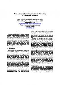
We illustrate in Figure 5 two possible results G” and G”’ of applying the rewrite rule r2 on the molecular graph G’. 1.2:EGF.EGF 1 1

2

5:EGFR

3

3.4:EGF.EGF

2

2

2 4

1

3

7:SHC

G'

2 4

2

1 1

2

1

6:EGFR

1

1.2:EGF.EGF 1 1

2

5:EGFR

3

3.4:EGF.EGF

2

2

2 4

1

3

7:SHC

2 4

2

1 1

2

1

6:EGFR

1

G"

1.2:EGF.EGF 1 1

2

5:EGFR

3

3.4:EGF.EGF

2

2

2 4

1

3

7:SHC

2 4

2

1 1

2

1

6:EGFR

1

G'''


Fig. 5. G” and G”’ are obtained from G’ by rewriting using the rule r2 on different subgraphs

Biological transformations as illustrated in the previous example have inspired many new computation models in recent years. In autonomic computing, systems and their components reconfigure themselves automatically according to directives (rewrite rules and strategies) given initially by administrators. Based on these primary directives and their acquired knowledge along the execution, an adaptive system seeks new ways of optimizing its performance and efficiency via new rewrite rules and strategies that it deduces; then it includes them in its own behavior. Since there is no ideal system, functioning problems and malicious attacks or failure cascades may occur, and the systems must be prepared to face them and solve them. The four most important aspects of self-management as presented in [17] are selfconfiguration, self-optimization, self-healing, and self-protection. In the strategic rewriting framework, the self-configuration is simply described by the concurrent application of the rules. A self-healing behavior can be described by rules that detect the problems and by rules that repair them by modifying the configuration or introducing new rules in the system. The same method can be used as well for self-optimization and self-protection as illustrated in [4]. In the next section, we define an abstract biochemical calculus for adaptive systems. Objects may be instantiated for instance as terms or as port graphs. Rules and strategies are first-class objects of the calculus. As a consequence, they can be rewritten as well, and rules can create new rules, providing a way of modeling adaptive systems.

3

The Abstract Biochemical Calculus

The calculus presented here is inspired by two previous works: the ρ-calculus (also called the rewriting calculus) [14] and the γ-calculus [6]. The ρ-calculus extends first-order term rewriting and the λ-calculus. From the λ-calculus, the ρ-calculus inherits higher-order capabilities and the explicit treatment of functions and their applications. Moreover, all the basic ingredients of rewriting are explicit objects, in particular the notions of rewrite rule (or abstraction), rule application, and structure of results. In the ρ-calculus, the usual λ-abstraction λx.t is replaced by a rule abstraction p _ t, where p and t are two ρ-terms, with p called a pattern, and the free variables of p are bound in t. Thus 7


Andrei and Kirchner

the ρ-calculus generalizes the λ-calculus by abstracting over a pattern instead of a simple variable. The chemical metaphor was proposed as a computational paradigm in the Γ language [8]. Computations are described in terms of a chemical solution in which molecules, representing data, interact according to reaction rules. Chemical solutions are represented by multisets and the reaction rules by rewrite rules on such multisets. Then the computation proceeds by application of rewrite rules which consume and produce new elements according to the conditions and transformations specified by the reaction rules. The chemical metaphor was used as well as a basis for defining the CHemical Abstract Machine (CHAM) [9]. The γ-calculus [6] was designed as a basic higher-order calculus developed on the essential features of the chemical paradigm. It generalizes the chemical model by considering the reactions as molecules as well. The Higher-Order Chemical Language (HOCL) [7] extends the γ-calculus with programming elements. The γ-calculus and HOCL were proved to be well-suited for modeling autonomous systems and for grid programming. A natural extension of the chemical metaphor is to enrich it with a biological flavor by providing the molecules with a particular structure and with association (complexation) and dissociation (decomplexation) capabilities. In living cells, molecules like nucleic acids, proteins, lipids, carbohydrates can combine based on their structural properties to form more complex entities. Biochemistry as science focuses heavily on the role, function, and structure of such molecules. Adding association and dissociation capabilities for molecules represents an essential feature for passing from a minimal chemical model to a biochemical one [12]. Along this line, we extend the chemical model by embedding higher-order capabilities of ρ-calculus and by considering an abstract structure OBJ for the molecules and for the computation rules. The structure OBJ permits the modeling of connections between objects as well as the actions of creating and removing such connections. The result is an abstract biochemical calculus based on rewriting structured molecules, called the ρhOBJ i -calculus and presented in the rest of this section. 3.1

Syntax

For OBJ a set of structured objects and X a set of variables, the syntax of the calculus is defined in Figure 6. (Objects)

O

::=

OBJ | X | O• O

(Molecules)

M

::=

O | O ⇒ O | M• M

(Configuration)

K

::=

M | M V M | K• K

(System)

S

::=

[K]

Fig. 6. The basic syntax of the ρhOBJ i -calculus

We consider collections of objects that are built out of structured objects and a juxtaposition operator that is supposed to be associative and commutative. We assume that this juxtaposition operator is not a constructor for the structured ob8

Andrei and Kirchner


jects. Molecules are bags, built once again using the same associative-commutative juxtaposition operator • as for objects, that contain not only collections of objects but also rules. Rules define transformations of collections of objects. Developing this calculus on a (bio)chemical metaphor, the juxtaposition operator simulates a kind of Brownian motion of objects and rules. We add a higher-order feature, the abstractions, which are necessary for expressing transformations over molecules. A rule can be seen as a first-order abstraction that transforms only (collections of) objects while the general higher-order abstractions act on objects and on rules as well. Collections of molecules and abstractions are called configurations. Then all molecules and abstractions are put in a collection to obtain a system, which we also refer to as (system) state. We introduce the system entity in order to distinguish between global and local configurations by making explicit the square brackets for the later ones. We distinguish the two types of transformations in the ρhOBJ i -calculus by defining the set of rules R and the set of abstractions A as below: (Rules)

R

::=

O⇒O

(Abstractions)

A

::=

MVM

Hereinafter, let us consider the symbol V ⇒ standing for ⇒ or V. By their definition, abstractions can specify not only transformations on objects but on rules as well, including deleting and creating rules. The next example illustrates our motivation for defining abstractions in addition to the usual rules specifying transformations on objects. Example 3.1 Let us consider a system where a protein ProteinBB is created from ComplexB via the rule ComplexB ⇒ ProteinBB . But the occurrence of a particular vitamin VitaminX changes the production of proteins ProteinBB from ComplexB to twice as much as in the conditions when VitaminX is not present in the system. In order to model this behavior, we include in the definition of the system the following abstraction: (VitaminX • (ComplexB ⇒ ProteinBB )) V (VitaminX • (ComplexB ⇒ ProteinBB • ProteinBB )) Application of this abstraction will transform the rule ComplexB ⇒ ProteinBB into ComplexB ⇒ ProteinBB • ProteinBB , but only in the presence of VitaminX . 3.2

Semantics

The evaluation mechanism of the calculus relies on the fundamental operation of matching. When applying an abstraction, this operation allows binding variables to their corresponding values. The general framework of the calculus allows matching to be performed syntactically or modulo a theory. The theory modulo which the matching is performed is thus a parameter of the calculus; we only suppose that there is a function Sol that returns the set of substitutions that are solution of a given matching problem between two molecules M and M 0 denoted M ≺≺ M 0 . 9

Andrei and Kirchner

(Interaction)

[K • (M V ⇒ N )• M 0 ] −→i [K • ς(N )] if ς ∈ Sol(M ≺≺ M 0 )


Fig. 7. The operational semantics of the ρhOBJ i -calculus

For the (Interaction) evaluation rule, we consider that a rule from R is applied only when no abstraction from A \ R is applicable. More precisely, a rule from L ⇒ R ∈ R in a system of the form [A1 • . . . • An • M ] with Ai in A \ R and L ⇒ R in M is considered by the (Interaction) evaluation rule only if ∀Ai = Li V Ri , we have Sol(Li ≺ ≺ M ) = ∅. This means that the application of abstractions has higher priority than application of rules. This calculus generalizes the λ-calculus, the γ-calculus and HOCL through a more powerful abstraction power that considers for matching not only a variable or a pattern from a restricted pattern language, but a more generic object built over an algebraic structure and a set of variables. The ρhOBJ i -calculus also encompasses the rewriting calculus [14] and the term graph rewriting calculus [10] by considering the tree-like structure of terms and the graph-like structure of termgraphs respectively as special structures. 3.3

Adding Strategies to the Biochemical Calculus

By considering the ρhOBJ i -calculus as a modeling framework for a system, we gain in expressivity by choosing convenient descriptions of the states, and we dispose of a great flexibility in modeling the system dynamics. For instance, rules can be consumed when applied and new rules can be created by the application of other rules. Then, instead of having a non-deterministic (and possibly non-terminating) behavior for the application of abstractions, one may want to introduce some control to compose or to choose the rules to apply. The notion of abstraction proves to be powerful enough to express such control, thanks to the notions of strategy and strategic rewriting. In addition, strategies allow exploiting failure information.

Rewrite Strategies as Abstractions In this section, we define strategies as objects of the calculus, using the basic constructs, as one can do in the λ-calculus or the γ-calculus. For such definition we use a similar approach to the one used in [15] where rewrite strategies are encoded by rewrite rules. Then, thanks to strategies, new extensions for the calculus are possible, for instance to catch a failure in the application or to define persistent strategies, as shown later. We first extend the syntax of the calculus with the failure or stuck object, stk. This failure object stk is the result of a failing application of an abstraction to a molecule as explained later in the semantic rules. In order to encode strategies, we also need to add to the calculus the notion of sequentiality. Therefore we introduce the application operator @ for applying an abstraction to a molecule to construct a reacting molecule and then for applying an abstraction on a reacting molecule. We obtain recursively new types of configurations. The syntax of the calculus with strategies is given in Figure 8. 10

Andrei and Kirchner

(Objects)

O

::=

stk | OBJ | X | O• O

(Molecules)

M

::=

O | O ⇒ O | M• M

(Configurations)

K

::=

M | M V K | (M V K)@K | K• K

(System)

S

::=

[K]

Fig. 8. The syntax of the ρhOBJ i -calculus with strategies

At this point of development of the calculus, the abstractions which we also call strategies may contain in their right-hand side the application construct:


(Abstractions) T ::= M V K The semantics of the calculus is given now as a set of four reduction rules (Figure 9) which take into account the application operator @ and failing abstraction applications. The evaluation rule (Interaction) chooses an abstraction M V ⇒ K and a molecule M 0 in the system and reduces them in the same way as it is done in the basic version of the calculus (see Section 3.2). In the case of reducing the application of an abstraction to a molecule, if a matching failure occurs during the application process, we handle it explicitly. If the matching problem between the left-hand side of the abstraction M V ⇒ K and the molecule M 0 has solutions, the evaluation rule (Application) is used and one substitution is chosen from the solution set and applied on the right-hand side of M V ⇒ K; otherwise, if the matching problem has no solution, the evaluation rule (Application Fail) is used and the application fails by returning the stk object. The evaluation rule (Stuck) removes any stk object from a juxtaposition of configurations. (Interaction)

[K 0 • (M V ⇒ K)• M 0 ] −→i [K 0 • ς(K)] if ς ∈ Sol(M ≺≺ M 0 )

(Application) (Application Fail) (Stuck)

(M V ⇒ K)@M 0 −→a ς(K) if ς ∈ Sol(M ≺≺ M 0 ) (M V ⇒ K)@M 0 −→f stk if Sol(M ≺≺ M 0 ) = ∅ stk• K −→s K

Fig. 9. The operational semantics of the ρhOBJ i -calculus with strategies

In the following we encode some usual strategies as built-in abstractions in the ρhOBJ i -calculus. Let us extend the set of object variables X to molecule variables. We consider for the strategy combinators enumerated in Section 2, the following abstractions (or aliases): id for Id, fail for F ail, first for F irst, seq for ; , not for N ot, ifThenElse for IfThenElse. These abstractions are defined using the extended 11

Andrei and Kirchner

syntax of Figure 9 and molecule variables. id , X V ⇒X fail , X V ⇒ stk seq(T1 , T2 ) , X V ⇒ T2 @(T1 @X) first(T1 , T2 ) , X V ⇒ (T1 @X)• (stk V ⇒ (T2 @X))@(T1 @X) not(T ) , X V ⇒ first(stk V ⇒ X, X 0 V ⇒ stk)@(T @X) ifThenElse(T1 , T2 , T3 ) , X V ⇒ first(stk V ⇒ T3 @X, X 0 V ⇒ T2 @X)@(T1 @X) The abstraction corresponding to the composed rewrite strategy T ry is then easily defined based on the strategies first and id, whereas for Repeat we use the recursion operator µ and the strategies try and seq as follows:


try(T ) , first(T, id) repeat(T ) , µX.try(seq(T, X)) We encode the µ abstraction using the fixed-point combinator of the λ-calculus as done for encoding iterators in the ρ-calculus [14]. In order to get the intended behavior of strategies, we impose in the ρhOBJ i calculus with strategies that no reduction is allowed in the right-hand side of an abstraction. Under this assumption, the encoding of rewrite strategies as abstractions in the ρhOBJ i -calculus is correct with respect to the semantics of abstract strategies as given in [18], in the following sense: Theorem 3.2 For every strategy T in the calculus obtained by combining the primitive strategy objects id, fail, seq, first, not, ifThenElse and for every molecule M , a successful reduction of T @M yields a configuration K such that K is obtained from M by strategic rewriting under the strategy T . Example 3.3 In the calculus of molecular graphs, for the system corresponding to the EGFR pathway fragment described in the previous example, the initial state is a world consisting of the molecular graph G and several strategies built upon the five reaction rules. G can be also written as the following juxtaposition of molecular graphs (or nodes in this particular situation): 1:EGF• 2:EGF• 3:EGF• 4:EGF• 5:EGFR• 6:EGFR• 7:SHC Let us consider a few examples of strategies for generating the biochemical network. The most straightforward way of modeling the biochemical network for the EGFR signaling pathway fragment presented here is to consider the juxtaposition of the reaction rules as persistent strategies. Hence the initial state of the system is the simple world [r1!• r2!• r3!• r4!• r5!• G]. Then any of the five rules is applied exhaustively. We can easily prove that the system will reach a stable state since with every successful rule application, either the total number of free and hidden sites decreases or if it remains constant (when applying rule r4) the number of hidden site decreases. 12

Andrei and Kirchner


The strategy first can be used to specify a higher priority in the application of two rules; for instance, first(r2 , r1 ) is saying that an EFG dimer binds to a receptor as soon as it is created. Then the initial state is [first(r2, r1)!• r3!• r4!• r5!• G]. We can slightly modify this state such that r3 is not persistent: [first(r2, r1)!• r3• r4!• r5!• G]. This means that the rule r3 is consumed when creating the active dimer RTK; having only one instance of such rule allows the creation of only one active dimer RTK. The execution can be separated in two stages: the first one is concerned with the extracellular interactions between the signals and the receptors, namely the reactions r1, r2 and r3, while the second one with the RTK pathway, namely the reactions r4, r5. If we consider that r2 has a higher application priority than r1, and any reaction from the first stage has an higher priority than any reaction from the second stage, then the initial world of the system is: [first(first(r2, r1), r3)• first(first(r2, r1), r4)• first(first(r2, r1), r5)• G] From every such initial state, the interactions lead to a state of equilibrium where no more rules can be applied. In each case, the equilibrium state contains either the molecular graph H given in Figure 10 or G”’ from Figure 5. 1.2:EGF.EGF 1 1

5:EGFR

7:SHC

2

1

3.4:EGF.EGF

2

2

2 4

2

3

3

2 4

2

1

1 1

6:EGFR

1

Fig. 10. The molecular graph H for the EGFR signaling pathway fragment in the equilibrium state

Failure Recovery Explicit failure provides the calculus with more expressivity. By considering a strategy with the failure object as the left-hand side, we can catch and tackle appropriately the failure of the application of another strategy. Based on the strategy definitions, we can reformulate the main reduction rule modeling the interaction between a strategy T and a molecule M using a failure catching mechanism: (InteractionR)

[K • T • M ] −→ir [K • seq(T, try(stk V ⇒ T • M ))@M ]

(1)

A reduction using the rule (1) proceeds in either of the following ways: •

if T @M reduces to the failure construct stk, then the strategy try(stk V ⇒ T •M ) restores the initial abstraction and molecule subject to reduction;

•

if T @M succeeds, then the application of the strategy try(stk V ⇒ T • M ) does not change the result of the application T @M .

We call this improved reduction interaction with recovery and stk V ⇒ T •M a recovery abstraction. The abstraction T and the molecule M from the right-hand side of the recovery rule cannot interact before the rule is applied thanks to the 13


Andrei and Kirchner

evaluation strategy which does not permit reduction inside the right-hand side of an abstraction. In the following we denote by −→∗ the reflexive and transitive closure of the relation −→=−→ir ∪ −→a ∪ −→f ∪ −→s . The behavior presented above for the interaction with recovery rule is correct under the assumption that the failure object stk is a protected symbol that cannot be introduced in a right-hand side of abstraction if it is not already present in the left-hand side. In other words, an user-defined abstraction M V ⇒ K may check whether the failure object stk is present in M but is not allowed to introduce it in K. This restriction is motivated by the following example. Let us take a user-defined abstraction O V ⇒ stk and an object O0 such that O matches O0 , then (O V ⇒ stk)@O0 reduces to stk. The abstraction is applied successfully but the result says that the application has failed. The contradictory situation comes from the use of the application failure information as an explicit object. This example shows that the expressive power we gained by making the failure an explicit object can lead to an unexpected behavior if not handled with caution. The interaction with recovery rule (1) is just an example of tackling a matching failure occurred in the application process. Instead of just recovering the interacting abstraction T and molecule M , one can imagine other ways of tackling a failure in the interaction, for instance by modifying M or even T . Persistent Strategies At this level of definition of the calculus, a strategy (and in particular a rule) is consumed by a non-failing interaction with a molecule M . One advantage is that, since we work with multisets, a strategy can be given a multiplicity, and each interaction between the strategy and a molecule M consumes one occurrence of the strategy. This permits controlling the maximum number of times an interaction can take place. Sometimes however it is suitable to have persistence of strategies. For this purpose, we define the persistent strategy combinator that applies a strategy given as argument and, if successful, replicates itself: T ! , µX.seq(T, first(stk V ⇒ stk, Y V ⇒ (Y • X))) Application of the strategy T ! to a molecule M leads to one of the two following situations: •

If T @M reduces to stk, the abstraction stk V ⇒ stk is applied; then the interaction with recovery rule reduces stk to the juxtaposition T !• M ;

•

If T @M reduces to a non-failing configuration K then the second argument of the strategy first is applied, Y is instantiated by K, and the final result is T !• K.

As for the encoding of the Repeat strategy, we use an encoding of the recursion operator µ as done for the ρ-calculus [14] and detailed in [1]. Based on the correctness of the encoding of the recursion operator µ as done for the ρ-calculus [14], the following result proves that the persistent strategy combinator is correctly defined in the ρhOBJ i -calculus with strategies. 14

Andrei and Kirchner

Proposition 3.4 Let M be a molecule and T an abstraction. If T @M −→∗ stk, then T !• M −→ir −→∗ T !• M , else, if T @M −→∗ K with K 6= stk, i.e., the application does not fail, then T !• M −→ir −→∗ T !• K. If we consider that a successful application of a strategy to a molecule does not consume the strategy, then the strategies are persistent by definition and we no longer need to define the persistent combinator for strategies. However, the current approach gives us the freedom of providing some strategies with a persistent behavior, while others exist in a limited number of occurrences, and are consumed after a few applications.


3.4

Coarse-Grained Reduction Relation

Before modifying the semantics of the calculus to take into account the invariant verification, we define another reduction relation coarser than the reduction relation defined in Figure 9. It consists of an interaction step, followed by application and possible stuck steps. At this coarse-grained level, we no longer focus on the internal processing of an interaction between a strategy and a molecule, but on its final result. Definition 3.5 [Evolution step] An evolution step for a system [K • T • M ] is a reduction consisting of the sequential composition of two stages: the first stage corresponds to reduction using the interaction with recovery rule (InteractionR), and the second stage to the union of the application rules (Application) and (Application Fail), and the stuck removing rule (Stuck). τ An evolution step is silent (or non-observable), denoted by −→, if the recovery rule stk V ⇒ T • M is applied during the second stage. In other words, the strategy T chosen to be applied on M fails. An evolution step is visible if it is not silent. Definition 3.6 [Coarse-grained one-step reduction of a system] A coarse-grained one-step reduction of a system is induced by finitely many silent evolution steps and T τ τ one visible evolution step. We denote it by Z⇒ or Z⇒ for (−→)∗ −→ and (−→)∗ −→T respectively if the successfully applied strategy T is relevant. Informally, the coarse-grained one-step reduction relation between a strategy T T and a molecule M states that: [K • T • M ] Z⇒ [K • M 0 ] if M 0 can be obtained from M by rewriting under the strategy T . We need such a coarse-grained reduction level in the ρhOBJ i -calculus in order to verify in Section 4 the invariance of a structural formula with respect to a modeled system. 3.5

Towards Embedding Verification in the Biochemical Calculus

The ρhOBJ i -calculus can be instantiated with the structure of port graphs presented in Section 2 to obtain a biochemical calculus for port graphs, which we call the ρpg -calculus. We have shown in [4] how a particular adaptive system can be modeled using the ρpg -calculus. The model should also ensure formally that the intended selfmanaging specification of the system helps indeed preserving its properties. Some 15


Andrei and Kirchner

of them can be verified by checking the presence of particular port graphs. This is the case if they are encoded as object port graphs, abstractions, or strategies, hence as entities of the calculus. Consequently, the properties can be placed at the same level as the specification of the modeled system and they can be tested for satisfiability at any time. For instance, embedding the self-healing property in a system modeled in ρpg -calculus can be performed by associating a recovery strategy for each strategy modeling a behavior of the system. Let recovery(T ) denote the recovery strategy for T . Then instead of T we have first(T, recovery(T )). If the recovery strategy is id then we obtain try(T ) which avoids a failure, whereas using fail as recovery strategy does not change the failure if the strategy T fails. Of course, what needs to be done is to determine which are the recovery strategies for each strategy of the system. A first approach for embedding verification in the model consists in expressing an invariant of the system as an abstraction with identical sides, M V ⇒ M , testing the presence of a molecule M . The failure of the invariant is handled by a failure port graph Error that does not allow the execution to continue. The strategy verifying such an invariant is then: first(M V ⇒ M, X ⇒ Error)! From another perspective, we express the unwanted occurrence of a object port graph G in the system using the strategy (G ⇒ Error)!. For instance in our running example on the EGFR signaling pathway fragment, an example of an undesirable pattern describes that the two dimers EGF.EGF are bound to different receptors, situation which prevents the two receptors to bound together and to be activated. In the next section we show how we can increase the expressivity of the ρpg -calculus by embedding a particular set of structural formulas in the syntax and adjusting correspondingly the reduction semantics in order to verify the formulas in parallel with the evolution of the modeled system.

4

Adding Invariants to the Biochemical Calculus

In the context of modeling adaptive systems, runtime verification is useful for recovering from problematic situations, i.e., for the self-healing property, or for adapting accordingly to changes in the environment or changes in the interacting parts. Typical requirements one may want a system to satisfy concern the occurrence, consequence or invariance of particular structural or behavioral properties. Such types of requirements are also interesting for verifying biochemical models [13,21]. In this paper we focus on verifying that particular structural properties of a modeled system are invariant. In this section we illustrate directly the principles of performing invariant verification on the structure of port graph in the ρpg -calculus. Nevertheless, this approach is valid for any kind of object structure OBJ provided that a free algebraic structure can be associated to OBJ . 16

Andrei and Kirchner

4.1

Structural Formulas

We call a port graph expression (or pattern) any port graph whose identifiers, node names or port names may be variables from X . Let σ : X → Int ∗ ∪ ∇ be a variable assignment from variables to constants for node identifiers, node names, and port names respectively. We usually denote by σ ∗ the extension of σ over port graph expressions. Based on the port graph expressions defined above and on the Boolean connectors, we introduce in the following the structural formulas we intend to verify on each state of a system. Definition 4.1 [Structural formulas] Given ∇X a p-signature, the set of structural formulas, denoted by FS(∇X ), is constructed inductively as follows: > and ⊥ are structural formulas;

•

any port graph expression γ is a structural formula;

•

if ϕ, ϕ1 , and ϕ2 are structural formulas, then ¬ϕ, ϕ1 ∧ ϕ2 , ϕ1 ∨ ϕ2 , ϕ1 → ϕ2 , and ϕ are structural formulas. (Structural formula) ::=

> | ⊥ | γ | ¬ϕ | ϕ1 ∧ ϕ2 | ϕ1 ∨ ϕ2 | ϕ1 → ϕ2 |

ϕ

◊

ϕ

◊

The Boolean operators >, ⊥, ¬, ∧, ∨, → are the usual operators from propositional logic for “true”, “false”, “not”, “and”, “or”, and “implies” respectively. requires that the property holds on a fragment or port The somewhere operator subgraph of the state. As already known, we can consider only the Boolean operators ⊥, ¬, and ∨; then combinations of these operators define the other Boolean operators, >, ∧, and →. Definition 4.2 [Structural satisfaction] The satisfiability of a structural formula ϕ ∈ FS(∇X ) by a port graph G, denoted by G |= ϕ, is defined inductively as follows: G |= >

G 6|=⊥

G |= γ ⇔ ∃σ. G ≡ σ ∗ (γ)

G |= ¬ϕ ⇔ G 6|= ϕ

G |= ϕ1 ∧ ϕ2 ⇔ G |= ϕ1 and G |= ϕ2

G |= ϕ1 ∨ ϕ2 ⇔ G |= ϕ1 or G |= ϕ2

G |= ϕ1 → ϕ2 ⇔ G 6|= ϕ1 or G |= ϕ2

G |=

◊

ϕ ⇔ ∃G0 v G. G0 |= ϕ

◊

Remark that a port graph expression γ is satisfied by a port graph G if they are isomorphic. G structurally satisfies a formula γ if γ matches a subgraph of G. Proposition 4.3 G |=

γ if and only if Sol(γ ≺≺ G) 6= ∅.

◊


◊

•

The following proposition states that the structural satisfaction of formulas is defined up to port graph isomorphism. Proposition 4.4 If G |= ϕ and G ≡ G0 then G0 |= ϕ. 17

Andrei and Kirchner

4.2

Syntax and Semantics of the ρpg -Calculus with Invariants

In the ρpg -calculus with invariants we now consider systems guarded by structural formulas: (Guarded systems)

S

::=

[K]ϕ

A structural formula is mapped to a strategy: assuming that any port graph expression γ can be seen as a port graph molecule in the calculus, we define the mapping τ from structural formulas to strategies (or extended abstractions) as follows: = id

τ (⊥)

= fail

τ ( γ)

= γ⇒γ

τ (¬ϕ)

= not(τ (ϕ))

◊

τ (>)

τ (ϕ1 ∧ ϕ2 ) = seq(τ (ϕ1 ), τ (ϕ2 ))

τ (ϕ1 ∨ ϕ2 ) = first(τ (ϕ1 ), τ (ϕ2 ))


τ (ϕ1 → ϕ2 ) = X ⇒ seq(τ (ϕ1 ), first(stk ⇒ X, τ (ϕ2 )))@X Lemma 4.5 Let ϕ be a structural formula in the calculus and G a port graph molecule. Then τ (ϕ)@G reduces either to G or to stk. Intuitively, if the application of the strategy encoding ϕ on a port graph G fails, then the formula is not satisfied by G. The following proposition shows the soundness and completeness of encoding structural formulas as strategies. Proposition 4.6 Let G be a port graph molecule and ϕ a structural formula in the calculus. Then: •

G |= ϕ if and only if τ (ϕ)@G −→∗ G;

•

G 6|= ϕ if and only if τ (ϕ)@G −→∗ stk.

We verify a structural formula only on molecules and not on configurations (hence nor on abstractions). This restriction is justified by the fact that such a verification is equivalent to a strategy application and strategies can only be applied on molecules. In order to verify structural formulas describing configurations, one need to extend the syntax and the semantics of the calculus with abstractions having configurations in their left-hand side. We define now the reduction relation Z=⇒ between guarded systems. For a modeled system where K is the initial configuration and ϕ a structural property satisfied by K, we start with the initial guarded system [K]ϕ . Informally the reduction relation corresponds to: [K]ϕ Z=⇒ [K 0 ]ϕ if [K] Z⇒ [K 0 ] and K 0 |= ϕ saying that, being in the system configuration K where the structural formula ϕ is satisfied, if K 0 is the configuration obtained in a coarse-grained one-step reduction from K and the formula is still satisfied in this new configuration, then the invariant still holds at this step of evolution. We have already shown how we can test the satisfiability of K 0 |= ϕ using a strategy application on K 0 . Therefore we formally define the coarse-grained reduction 18

Andrei and Kirchner

relation using strategies as follows: [K]ϕ Z=⇒ ifThenElse(τ (ϕ), X1 V [K 0 ]ϕ , X2 V error message)@K 0 if [K] Z⇒ [K 0 ] If τ (ϕ)@K 0 reduces to a configuration different from stk (i.e., K 0 |= ϕ), then the state [K 0 ] is returned guarded with the same invariant property ϕ; otherwise, an error message is returned. Moreover, instead of an error message, we can return the state [K 0 ] guarded by the negated formula: [K 0 ]¬ϕ . Example 4.7 Let us consider a biological system where a virus (described by the pattern Virus) may intrude, but an antiviral drug (Antiviral ) can also be created. We then guard the system with the structural formula:


ϕ = ¬Virus ∨ (Virus ∧ Antiviral ) saying that either the virus is not present or the virus is present together with an antiviral drug. In the case the system reaches a state where the formula is not satisfied, we consider the negation of ϕ as guard of the system. Then the guard will be equal to ¬ϕ = Virus ∧ ¬Antiviral .

5

Conclusion and Future Work

The main original contributions of this paper are first to provide an abstract biochemical calculus to model systems evolving according to initial rules and strategies, that may in turn create new rules according to generated states; second, to show how to slightly extend the syntax in order to embed in the same calculus the verification of invariant properties of the system. When the objects of the calculus are instantiated by port graphs, we get an expressive representation of adaptive systems with interacting components, strongly inspired by biological systems. We hope that this work contributes to the theoretical understanding of autonomic computing. A further step going on is to have an implementation of the port graph calculus in which the user can visualize objects, rules and strategies, as well as the different states of a given system and history of its evolution. Even if the underlying concepts of graph rewriting have been largely explored, important problems remain to get a realistic implementation: efficiency issues of rewriting, huge graphs representation, dynamic reconfiguration of drawings are examples of problems we are addressing in the Porgy project, led as a collaboration between INRIA and King’s College (see Porgy Project homepage for more details). On the verification side there are also interesting perspectives to investigate further on. In particular, we can generalize the ideas presented in this paper as follows. Instead of yielding the failure Error or an error message for signaling that an invariant of the system is no longer satisfied, the problem can be “repaired” by associating to each invariant the necessary rules or strategies to be inserted in the system in case of failure. As we have already seen in this paper, for the biochemical calculus with invariants, a failure can be tested by the unsatisfaction of a structural formula. Then, as soon as the formula is unsatisfiable, a reparation rule may come into play by removing the unsatisfied formula, by modifying some molecules or strategies 19

Andrei and Kirchner

from the current state, or even by adding a new formula for guarding the execution from that state on. In order to be able to perform all these kinds of modifications, a solution would be to extend the definition of abstractions with structural formulas for each side to obtain guarded abstractions: M/ϕ1 V K/ϕ2 . For applying the abstraction M/ϕ1 V K/ϕ2 on [K1 ]ϕ , the matching problem M ≺≺ K1 should have a solution ξ which is also (or can be extended to) a solution for ϕ1 ≺≺ ϕ; the result of the abstraction application would consist of (i) removing the ξ-instantiated formula ϕ1 from the guard ϕ, (ii) applying the abstraction M V K based on ξ to obtain a state [K2 ], and (iii) adding the instantiated formula ϕ2 to the guard to obtain the formula ϕ0 ; if K2 |= ϕ0 then we could say that [K1 ]ϕ reduces to [K2 ]ϕ0 . An example of a guarded abstraction well-suited for Example 4.7 is the following: X/Virus∧¬Antiviral V ⇒ XAntiviral /¬Virus


which introduces an antiviral drug in the system to inhibit the development of the virus. This idea of extending the calculus is worth exploring since this would open a wide field of possibilities for combining verification and self-healing in ρpg -calculus.

References [1] Andrei, O., “A Rewriting Calculus for Graphs: Applications to Biology and Autonomous Systems,” Ph.D. thesis, Institut National Polytechnique de Lorraine, Nancy, France, 2008. URL http://tel.archives-ouvertes.fr/tel-00337558/fr [2] Andrei, O. and H. Kirchner, Graph Rewriting and Strategies for Modeling Biochemical Networks., in: SYNASC ’07: Proceedings of the Ninth International Symposium on Symbolic and Numeric Algorithms for Scientific Computing (2007), pp. 407–414. URL http://dx.doi.org/10.1109/SYNASC.2007.44 [3] Andrei, O. and H. Kirchner, A Rewriting Calculus for Multigraphs with Ports., in: Proceedings of RULE’07, Electronic Notes in Theoretical Computer Science 219, 2008, pp. 67–82. [4] Andrei, O. and H. Kirchner, A Higher-Order Graph Calculus for Autonomic Computing, in: M. a. Lipshteyn, editor, Graph Theory, Computational Intelligence and Thought. Golumbic Festschrift, Lecture Notes in Computer Science 5420 (2009), pp. 15–26. [5] Balland, E., P. Brauner, R. Kopetz, P.-E. Moreau and A. Reilles, Tom: Piggybacking rewriting on java, in: Proceedings of the 18th Conference on Rewriting Techniques and Applications, Lecture Notes in Computer Science 4533 (2007), pp. 36–47. [6] Banˆ atre, J.-P., P. Fradet and Y. Radenac, Higher-Order Chemical Programming Style, in: J.-P. Banˆ atre, P. Fradet, J.-L. Giavitto and O. Michel, editors, UPP, Lecture Notes in Computer Science 3566 (2004), pp. 84–95. [7] Banˆ atre, J.-P., P. Fradet and Y. Radenac, Programming Self-Organizing Systems with the Higher-Order Chemical Language, International Journal of Unconventional Computing 3 (2007), pp. 161–177. [8] Banatre, J.-P. and D. L. Metayer, A New Computational Model and Its Discipline of Programming., Technical Report RR-566, INRIA (1986). [9] Berry, G. and G. Boudol, The Chemical Abstract Machine., Theoretical Computer Science 96 (1992), pp. 217–248. [10] Bertolissi, C., P. Baldan, H. Cirstea and C. Kirchner, A Rewriting Calculus for Cyclic Higher-order Term Graphs., Electronic Notes in Theoretical Computer Science 127 (2005), pp. 21–41. [11] Borovansk´ y, P., C. Kirchner, H. Kirchner and C. Ringeissen, Rewriting with strategies in ELAN: a functional semantics, International Journal of Foundations of Computer Science 12 (2001), pp. 69–98. [12] Cardelli, L. and G. Zavattaro, On the Computational Power of Biochemistry, in: K. Horimoto, G. Regensburger, M. Rosenkranz and H. Yoshida, editors, AB’08, Lecture Notes in Computer Science 5147 (2008), pp. 65–80.

20

Andrei and Kirchner [13] Chabrier-Rivier, N., F. Fages and S. Soliman, The Biochemical Abstract Machine BIOCHAM., in: V. Danos and V. Sch¨ achter, editors, Computational Methods in Systems Biology, International Conference CMSB 2004, Paris, France, May 26-28, 2004, Revised Selected Papers, Lecture Notes in Computer Science 3082 (2005), pp. 172–191. [14] Cirstea, H. and C. Kirchner, The Rewriting Calculus - Part I and II, Logic Journal of the IGPL 9 (2001), pp. 427—498. [15] Cirstea, H., C. Kirchner, L. Liquori and B. Wack, Rewrite strategies in the rewriting calculus., Electronic Notes in Theoretical Computer Science 86 (2003), pp. 593–624. [16] Danos, V. and C. Laneve, Formal Molecular Biology., Theoretical Computer Science 325 (2004), pp. 69– 110. [17] Kephart, J. O. and D. M. Chess, The Vision of Autonomic Computing, IEEE Computer 36 (2003), pp. 41–50. [18] Kirchner, C., F. Kirchner and H. Kirchner, Strategic computations and deductions, in: C. Benzmueller, C. E. Brown, J. Siekmann and R. Statman, editors, Reasoning in Simple Type Theory: Festschrift in Honor of Peter B. Andrews on His 70th Birthday (Paperback), Studies in Logic, Mathematical Logic and Foundations 17 (2008), pp. 339–364. [19] Laneve, C. and F. Tarissan, A simple calculus for proteins and cells., Electronic Notes in Theoretical Computer Science 171 (2007), pp. 139–154.


[20] Mart´ı-Oliet, N., J. Meseguer and A. Verdejo, A Rewriting Semantics for Maude Strategies., Electronic Notes in Theoretical Computer Science 239 (2009), pp. 227–247. [21] Monteiro, P. T., D. Ropers, R. Mateescu, A. T. Freitas and H. de Jong, Temporal logic patterns for querying dynamic models of cellular interaction networks, Bioinformatics 24 (2008), pp. 227–233. [22] Visser, E., Stratego: A Language for Program Transformation based on Rewriting Strategies. System Description of Stratego 0.5., in: A. Middeldorp, editor, Rewriting Techniques and Applications (RTA’01), Lecture Notes in Computer Science 2051 (2001), pp. 357–361.

21