This is the second paper detailing a new Maple package for graph theory, called ..... From König's theorem we know that the chromatic index of every bipar-.
A Graph Theory Package for Maple, Part II: Graph Coloring, Graph Drawing, Support Tools, and Networks. Mohammad Ali Ebrahimi, Mohammad Ghebleh, Mahdi Javadi Michael Monagan and Allan Wittkopf Department of Mathematics, Simon Fraser University, 8888 University Drive, Burnaby, BC, Canada V5A 1S6. {mebrahim,mghebleh,mmonagan,sjavadi,wittkopf} @cecm.sfu.ca
1
Introduction
This is the second paper detailing a new Maple package for graph theory, called GraphTheory, [3], that is being developed at Simon Fraser University as part of our MITACS research project. The package is intended for both research and teaching. It supports directed and undirected graphs, weighted and unweighted graphs, and networks, but not multigraphs. The package includes procedures for drawing graphs in 2 and 3 dimensions. To make the package easy to use we have added Maple style ‘context menus’. This provides access to many of the commands in the package via using menus and the mouse. In this paper we describe new functionality added to support graph input, storing of arbitrary information about edges and vertices, importing graphs from and exporting graphs to other software, including support for MetaPost for use with LATEX. We describe a graph drawing algorithm that models a graph as a physical system that leads to a system of second order differential equations that needs to be solved. This approach gives very good drawings of graphs. It is limited in that its complexity is inherently O(n2 ) where n is the number of vertices in the graph. Our implementation is effective for n up to about 100. We also describe the facilities for graph coloring and for networks. There are many texts on graph theory. The primary algorithms reference that we have used was Introduction to Algorithms by Cormen, Leiserson, Rivest and Stein. See [1]. Also [8], Gabriel Valiente’s Algorithms on Trees and Graphs which focusses on the graph isomrophism problem. Another good text devoted
1
to graph theory algorithms is [4], Dieter Jungnickel’s Graphs, Networks, and Algorithms.
2 2.1
Defining Graphs The Graph and Digraph commands
The commands Graph and Digraph are used to construct an undirected or directed graph, respectively. Here we describe the Graph command. The following parameters of the graph can be given in any order as arguments of the Graph command: number of vertices, vertex labels, edges/arcs, the adjacency matrix, the weight matrix, the keywords directed, undirected, weighted, and unweighted. Vertex labels are specified in a list (in a fixed order). Each label can be either an integer, a symbol, or a string. Edges are of the form {x,y} and arcs are of the form [x,y] where x and y are valid vertex labels. A convenient solution for entering the edges of a graph is to use trails. For example Trail(1,2,3,4,2,3,5) for an undirected graph is short for the edges {{1,2},{2, 3},{3,4},{2,4},{3,5}}. If the graph to be constructed is weighted, then the weights of edges/arcs can be given in a weight matrix, or in the set of edges in the form [e,w], where e is an edge/arc and w is the weight of e. If no weight is assigned to an edge, it is assigned the weight 1 by default. Here are some examples. > G := Graph(5); Graph 1 : an undirected unweighted graph with 5 vertices and 0 edge(s) > Vertices(G), Edges(G); [1, 2, 3, 4, 5], {} > Graph([a,b,c,d,e], {{a,b}, {b,c}, {c,e}, {a,c}}); Graph 2 : an undirected unweighted graph with 5 vertices and 4 edge(s) > Graph({{a,b}, {b,c}, {c,e}, {a,c}}); Graph 3 : an undirected unweighted graph with 5 vertices and 4 edge(s) > G := Graph([a,b,c,d,e], Trail(c,a,b,c,e)); G := Graph 5 : an undirected unweighted graph with 5 vertices and 4 edge(s) > Edges(G); {{c, a}, {c, b}, {c, e}, {a, b}} > W := Matrix(6, {(1,2)=2,(2,3)=4,(2,6)=7,(3,4)=6,(3,5)=5,(4,5)=3}, shape=symmetric): > G := Graph([$1..6], W): > Edges(G, weights); {[{1, 2}, 2], [{2, 3}, 4], [{2, 6}, 7], [{3, 4}, 6], [{3, 5}, 5], [{4, 5}, 3]}
2
> A := Matrix([[0,1,1,1],[1,0,1,0],[1,1,0,1],[1,0,1,0]]); > Edges( Graph([a,b,c,d], A) ); {{a, b}, {a, c}, {a, d}, {b, c}, {c, d}} A graph may also be defined by specifying its list of neighbors. This argument must be of type list or Array of sets of vertices. For example: > A := Array([{2,3}, {1,3,4,5}, {1,2,4,5}, {2,3}, {2,3}]); > Edges( Graph([v1,v2,v3,v4,v5], A) ); {{v1, v2}, {v1, v3}, {v2, v3}, {v2, v4}, {v2, v5}, {v3, v4}, {v3, v5}}
2.2
The data structure
The GraphTheory package stores graphs in Maple as functions. The following is the general form of a graph generated by the GraphTheory package: GRAPHLN(dir, wt, vlist, listn, ginfo, ewts) In this structure, dir and wt are symbols indicating whether the graph is directed or undirected and whether it is weighted or unweighted. The argument vlist is the list of vertex labels of the graph. Each label can be of type integer, string or symbol. Internally, the vertices are labelled by numbers 1, 2, . . . , n where n is the number of vertices of the graph. The adjacency structure of the graph is stored in listn which is an Array of sets. The ith entry in listn is the set of neighbors of the ith vertex. If the graph is weighted, the edge weights are stored in ewts which is of type Matrix. Additional information such as vertex positions and vertex and edge information will be stored in ginfo which is a of type table. The choice of ‘list of neighbors’ as the graph data structure provides makes it efficient to insert and delete new edges in a graph but adding and removing vertices is more expensive – it requires making a copy of the graph structure. Another restriction of the list of neighbors as the graph structure is that multiple edges are not supported.
2.3
Attributes
Using attributes, the user may attach arbitrary information to the graph, its vertices, and edges. Each attribute is an equation of the form tag = value. We illustrate with examples. > > > >
G := Graph( Trail(a, b, c, d, b) ): SetVertexAttribute(G, b, msg="text"); SetVertexAttribute(G, c, [msg="message", timesvisited=10]); GetVertexAttribute(G, c, timesvisited); 10 > GetVertexAttribute(G, b, timesvisited); FAIL > SetEdgeAttribute(G, {a,b}, msg="weak edge"); 3
> SetEdgeAttribute(G, {c,d}, [tag=fake,visited=true,cost=3]); > DiscardEdgeAttribute(G, {c,d}, tag); > GetEdgeAttribute(G, {c,d}); [visited = true, cost = 3]
2.4
Special graphs
The definitions of some special graphs are included in the SpecialGraphs submodule of the GraphTheory package. The following is a list of these special graphs. ClebschGraph CompleteBinaryTree CompleteGraph CompleteKaryTree CycleGraph DesarguesGraph DodecahedronGraph DoubleStarSnark DyckGraph FlowerSnark FosterGraph GeneralizedPetersenGraph GoldbergSnark
2.5
GridGraph GrinbergGraph GrotzschGraph HeawoodGraph HerschelGraph HypercubeGraph IcosahedronGraph KneserGraph LCFGraph LeviGraph MobiusKantorGraph OctahedronGraph OddGraph
PappusGraph PathGraph PayleyGraph PetersenGraph PrismGraph ShrikhandeGraph SoccerBallGraph SzekeresSnark TetrahedronGraph TorusGridGraph WebGraph WheelGraph
Context menu
The context menu is a convenient way to access some of the GraphTheory package commands. The context menu of a graph can be accessed in the Maple graphical user interface by right-clicking on the graph. An example is depicted in the following figure.
4
3
Drawing Graphs
The GraphTheory package provides a command DrawGraph for drawing graphs and digraphs. If a graph doesn’t contain drawing information, it is checked for being a tree or a bipartite graph in which cases it is drawn with respect to those structures. Otherwise the vertices are positioned on a circle. To force a style of drawing, one may specify a second argument which is of the form style=· · · In the remainder of this section we describe one of these styles, namely the spring style. The spring method may be used to generate 2-dimensional or 3-dimensional drawings of a graph. The default dimension is 2 and an extra argument dimension=3 can be used to generate a 3D drawing. Once a drawing is generated it will be stored in the memory for future reference. To force generation of a new drawing, which is useful for the spring method which uses random initial positions, one may use the option redraw in the DrawGraph command. Let G be a connected graph with n vertices V and m edges E. We want our algorithm to find an aesthetic layout of the graph that clearly conveys its structure and assign a location for each vertex and a route for each edge, so that the resulting drawing is ‘nice’. The method we use models a graph as a physical system that leads to a system of second order differential equations that must be numerically solved. We model edges in the graph with springs with zero rest length. We model vertices as nonphysical objects that exert a constant repulsive force on each of the other vertices. And we add damping to the physical system to dampen oscillations. Note that different variants of the differential equation spring model have been used, including springs with nonzero rest lengths [2], [5] modification of this method by an additional effect, temperature [6] as well as methods that dynamically change the model parameters as the system is integrated [7]. Thus we construct a system of second order differential equations where the equation for vertex i is the following: X X Xi (t) − Xj (t) d d2 cij Xi (t) = aij (Xi (t) − Xj (t)) − bi Xi (t) + 2 dt dt |Xi (t) − Xj (t)| j∈V
j∈N(i)
where V is the set of vertices of G, N (i) are the vertices adjacent to vertex i, Xi is the position of vertex i, a vector, and aij ,bi ,cij are constants that must be defined for the problem. Thus if there are n vertices in the graph and we model the system in 2 dimensions, there are 2n second order differential equations in 2n unknowns. For the initial values, we set initial velocities to 0 and choose initial positions at random inside the unit square (in 2 dimensions) and unit box (in 3 dimensions). This ode system must then be integrated until it reaches a steady state. This is accomplished by use of an externally implemented fourth-order Runge-Kutta method with the graph ode system built-in. It is informative to note that the original model in use was a more physical model, in that the repulsive force obeyed an inverse square law. Alas, we 5
found that use of this approach caused the computation to lock-up before an aesthetically pleasing graph was obtained (nodes could not cross one-another), suffered from rather severe issues with respect to asymptotic behavior (the equilibrium was slow to reach), and sometimes resulted in a sub-optimal steady state (e.g. the natural description of a wheel graph with many vertices is an unstable equilibrium with respect to the inverse square law). Finally, since a constant force model is in use, it is possible that the steady state can have overlapping vertices. To alleviate this problem, a post-processing integration is performed that steadily increases the repulsive force between overlapping vertices until they no longer overlap. While graph drawing is a complicated problem in general, an advantage of this approach is that it requires no special knowledge about the structure of the graph such as whether it has articulation points or not. It also gives very good drawings of graphs. It is limited in that the complexity is at least O(n2 ). This is because the model of vertices being charged particles repelling each other means each differential equation has n non-zero terms in it. Our implementation can treat graphs with n up to 100 in a few seconds. Damping Constants In order to reconstruct good graphs from the randomly positioned initial vertices it is important that the spring model is neither over damped nor under damped. Since we are solving the system of differential equations numerically, reaching the steady state takes significantly more effort if the damping is not optimal. To avoid this difficulty, we choose the damping constants (bi ), spring constants (aij ), and repulsion constants (cij ) carefully. After experimenting with different graphs we have concluded that the constants must depend upon characteristics of the graph. After some analysis, reasonable approximations for the optimal constants have been obtained, and the approach used is briefly outlined here. We have three sets of constants, and want to control three aspects of the problem: the time scale on which the steady state is reached, the length scale at the steady state, and the damping. With this in mind, we found the following relationships for the constants aij =
√ cae ae , bi = b a, cij = 1 , ei ej n pd (n d )
where e is the total number of edges in the graph, ei is the number of edges connected to vertex i, n is the total number of vertices in the graph, d is the number of dimensions the graph is being drawn in, pd (x) is a degree d + 2 polynomial in x, and a,b,c are constants that control the time scale, length scale, and damping for the problem. Note that the pd (x) polynomial simply describes the repulsive force of n uniformly distributed vertices in a 1 × 1 square (for 2-d) or a 1 × 1 × 1 cube (for 3-d) as measured at the center of any of the boundaries of the square/cube.
6
At this point, values for a,b,c were experimentally determined for the two and three dimensional cases, and it was found that fixed values for these provide very reasonable performance for a wide variety of graphs. The first example shows that the algorithm recovers the ‘wheel graph’. The graph on the left was constructed by placing all vertices in a circle using the command DrawGraph(G,style=circle). The graph on the right is using the algorithm. The command is DrawGraph(G,style=spring). 0
10 9 8
8
0
3
3
9
2
4 6
7
4
2
7
6
5
1
10
1
5
In this second example, we have constructed the Petersen graph. The graph on the right below is the default output of the DrawGraph command. This is usual way of drawing the Petersen graph. To obtain this output, the GraphTheory package stores the vertex positions for this special graph. The graph on the left is the output of the spring algorithm. It is another symmetric drawing of the Petersen graph. 7
3
1
6
6
10 5
4
2
8
9
2
9
1 8
10
5
4
7 3
The final two examples are in three dimensions. The spring algorithm is easy to generalize to higher dimensions. In three dimensions, it is possible that the orientation of the result, of say the wheel graph, would end up showing as a line. To prevent this from happening, we rotate the graph through various angles and choose the orientation which maximizes the area of the convex hull of the vertices when projected onto the viewing plane. The first example is a docdecahedron. This graph has 20 vertices and 30 edges.
7
4 9
5
3
13 2
19
18 15
12
7
14
10
8
20
17 11
16
The second example is a graph of a soccer ball. The surface of a soccer ball consists of pentagons and hexagons. There are 60 vertices and 90 edges. The spring algorithm recovered the soccer ball in 0.546 seconds on an AMD 64 bit Opteron running at 2.2 GHz. 1 6 10
8
3 4 15
5 12
20 18 19
14
59
58
38 60 39 37
24
53
28
29
55
52 47
57 43
44 51
46
4
17
54
30
49 48 50
16 21
13
26
7 9
2 11
56 36 35 42
45 34 33
31
41 32
Graph Coloring
There are several commands implemented in the GraphTheory package for dealing with graph coloring problems. Since coloring problems are NP-Complete in general, the commands usually use brute-force search methods. The two commands ChromaticNumber and ChromaticIndex return the chromatic number and the chromatic index (edge chromatic number) of a graph respectively. These commands also return an optimal coloring. To speed up the search, these commands calculate upper and lower bounds on the chromatic number of the given graph. The upper bound is obtained from a greedy colorn for ing of the graph while the lower bound is the maximum of ω(G) and α(G) a graph G where n is the number of vertices, ω(G) is the clique number, and α(G) is the independence number of G. The call ChromaticNumber(G, bound) calculates and returns the bounds without searching for the chromatic number. The commands IsKColorable and IsKEdgeColorable can be used to check if a graph is k-colorable or edge k-colorable for a fixed number k. 8
Circular colorings of graphs are also supported in the GraphTheory package. The commands CircularChromaticNumber and CircularChromaticIndex return the circular chromatic number and the circular edge chromatic number of a given graph along with the corresponding optimal circular colorings. The commands IsKDColorable and IsKDEdgeColorable are used to check (k, d)colorability or edge (k, d)-colorability for a fixed pair (k, d) of integers. From K¨ onig’s theorem we know that the chromatic index of every bipartite graph is equal to the maximum degree of a vertex in the graph. This theorem gives a polynomial-time algorithm for obtaining an optimal edge coloring of a bipartite graph. This algorithm is based on the maximum bipartite matching algorithm implemented in the GraphTheory package in the command BipartiteMatching. The ChromaticIndex command uses this method to obtain optimal edge colorings of bipartite graphs in polynomial time. These commands along with the ImportGraph and ExportGraph commands, and definitions of some families of snarks in SpecialGraphs, provide a good collection of tools for teaching and research in graph coloring.
5
Networks
There are four commands in the GraphTheory package for dealing with networks. They are IsNetwork, RandomNetwork, MaxFlow and DrawNetwork. Here we define a network to be a directed graph with at least one source and one sink. A source is a vertex of the network with no incoming arcs and a sink is a vertex with no outgoing arcs. The command IsNetwork is used to test whether a graph is a network or not. The command can also be used to determine whether a graph with two specified sets of vertices as sources and sinks is a network or not. > N := Digraph({[a,b], [c,d], [b,d], [d,e]}); N := Graph 1 : a directed unweighted graph with 5 vertices and 4 arc(s) > IsNetwork(N); true, {c, a}, {e} > IsNetwork(N, a, d); false > IsNetwork(N, c, e); true
5.1
Generating Random Networks
The command RandomNetwork can be used to create a random network with specified set or number of vertices. The generated Network has exactly one source and one sink. We partition the vertices of the network into levels. The source and sink are in the first and last levels respectively. If u and v are two vertices in the
9
network, if there is an arc from u to v and u belongs to the ith level then v must be in the (i + 1)st level. The user can specify the number of levels in the generated network with an argument p which is a number between 0 and 1. The larger p is, the larger the number of levels will be. For example for p = 1 the number of levels would be exactly the number of vertices and the ith level will only has the ith vertex as its member. There is also an optional argument q which determines the probability of having an arc between each pair of vertices. The generated network can be forced to be weighted or acyclic by adding each of these terms in the list of arguments. > N := RandomNetwork(10, 0.3); > IsNetwork(N); true, {1}, {10} > N := RandomNetwork(10, 0.3, acyclic, weighted); > IsNetwork(N); true, {1}, {10} > MaxFlow(N, 1, 10); 1.119382241
5.2
Drawing Networks
The GraphTheory package includes a command named DrawNetwork for displaying networks. The user can specify the set of vertices for sources and sinks of the network, otherwise the sets of all possible sources and sinks will be chosen. The user can also choose the network to be displayed either horizontally or vertically. > N := RandomNetwork(10, 0.3, .4, acyclic); N := Graph 2 : a directed unweighted graph with 10 vertices and 34 arc(s)! > DrawNetwork(N);
10
1
2
3
7
4
8
5
6
9
10
6
The ImportGraph and ExportGraph Commands
The ImportGraph and ExportGraph commands provide a way to read graphs from files into the GraphTheory package and to output graphs to files in some formats. One format is used in the DIMACS graph coloring challenge. For example the command ExportGraph(SpecialGraphs:-CycleGraph(5), "C5.col", dimacs) generates a file C5.col in the current working directory with the following content: c p e e e e e e e e e e
Generated by the Maple GraphTheory package edge 5 10 2 3 3 2 1 2 2 1 3 4 4 3 1 5 5 1 4 5 5 4
This file may be read into the GraphTheory package using the command ImportGraph("C5.col", dimacs). Another format supported by the ImportGraph and ExportGraph commands is the format used by the Mathematica package “Combinatorica”.
11
ExportGraph also supports export to MetaPost. The resulting file may be compiled using the mpost command (in Unix systems, for other systems refer to your LATEXmanual). Figure 1 shows the final result of the following commands. > G := SpecialGraphs:-DoubleStarSnark(); > ExportGraph(G, "dblstar.mp", metapost); 1
2
3
16 17 18
15 14
4
30 29 28
13
27
5
19 20 21
26
25
24
23
6
22
12
7 11
8 10
9
Figure 1: The double-star snark exported to MetaPost The MetaPost file generated by ExportGraph may be edited to customize the result. For example one may remove some vertex labels or change the size of the vertices.
References [1] T. Cormen, C. Leiserson, R. Rivest and C. Stein. Introduction to Algorithms, second edition, MIT Press, 2001. [2] P. Eades. A heuristic for graph drawing, Congressus Numerantium, 42:149– 160, 1984. [3] J. Farr, M. Khatirinejad, S. Khodadad, M. Monagan. A Graph Theory Package for Maple, Proceedings of the 2005 Maple Conference, pp. 260-271, Maplesoft, 2005. [4] Dieter Jungnickel. Graphs, Networks and Algorithms, Algorithms and Computations in Mathematics Series, Volume 5, Springer-Verlag, 1999.
12
[5] T. Kamada, S. Kawai, An algorithm for drawing general undirected graphs 31(1):7–15, 1989. [6] T. M. J. Fruchterman, E. M. Reingold. Graph Drawing by Force-directed Placement, Software - Practice and Experience, 21(11):1129–1164, 1991. [7] Xuejun Liu, Buntarou Shizuki, Jiro Tanaka. Dynamic Parameter Spring Modeling Algorithm for Graph Drawing, Proc. Intl. Symp. Future Software Tech. (ISFST2001), pp. 52–57, 2001. [8] Gabriel Valiente. Algorithms of Trees and Graphs Springer-Verlag, ISBN 3-540-43550-6, 2002.
13