Sep 16, 2013 - nique also allows us to prove some new bounds on graph products. .... G = G ⦠H where G ⦠H denote the rooted product of graph G and H, and ...
Coloring Graph Powers: Graph Product Bounds and Hardness of Approximation Parinya Chalermsook∗
Bundit Laekhanukit†
Danupon Nanongkai‡
September 16, 2013
Abstract We consider the question of computing the strong edge coloring, square graph coloring, and their generalization to coloring the k th power of graphs. These problems have long been studied in discrete mathematics, and their “chaotic” behavior makes them interesting from an approximation algorithm perspective: For k = 1, it is well-known that vertex coloring is “hard” and edge coloring is “easy” in the sense that the former has an n1−� hardness while the latter √ admits a (4/3)-approximation algorithm. However, vertex coloring becomes easier (can be O( n)-approximated) for k = 2 while edge coloring seems to become much harder (no known O(n1−� ) approximation algorithm) for k ≥ 2. In this paper, we show several new hardness of approximation results that clarify the approximability landscape of these problems. First, we confirm that edge coloring indeed becomes computationally harder when k > 1: we prove a hardness of n1/3−� for k ∈ {2, 3} and n1/2−� for k ≥ 4 (previously, only NP-hardness for k = 2 is known). Moreover, for vertex coloring, we prove a hardness of n1/2−� for all k, which is tight for all even k. We also prove hardness of maximum clique and stable set (a.k.a. independent set) problems on graph powers. These results rely on a common simple technique of proving bounds via fractional coloring. This technique also allows us to prove some new bounds on graph products. In addition, we include our proof of Erd¨ os and Neˇsetˇril conjecture on cographs using a charging scheme technique.
1
Introduction
Consider the following broadcast scheduling problem commonly considered in the network area (e.g. [27, 4, 19]). We are given a graph G representing a network of transceivers (represented by nodes). Each transceiver can send a message to its neighbors by broadcasting via some communication channel; however, two transceivers that share a neighbor cannot broadcast on the same channel since their signals interfere with each other. The objective is to minimize the number of channels we have to assign the transceivers to avoid interference. Formally, for any graph G = (V, E), we want a minimum value of C such that there is a function c : V → {1, . . . , C} where, for any pair (u, v) of vertices of distance at most two, c(u) 6= c(v). ∗
Max-Planck-Institut f¨ ur Informatik, Saarbr¨ ucken, Germany The work was partially done while the author was at IDSIA, Lugano, Switzerland. Supported by the Swiss National Science Foundation project 200020 144491/1 † School of Computer Science, McGill University, Canada Supported by the Natural Sciences and Engineering Research Council of Canada (NSERC) grant no. 429598 and by Dr&Mrs M.Leong fellowship. ‡ Nanyang Technological University, Singapore
1
In theoretical computer science and discrete mathematics, this problem is known as distance-2 vertex coloring or coloring square graphs (e.g., [22, 25, 1, 2, 18]) – we simply view the channel assignment as a color assignment. Its natural extension, distance-k coloring or coloring the k th power graphs is also extensively studied (e.g., [2, 25, 1, 18]). Formally, denote by Gk the k th power of a graph G and χ(G) its chromatic number. Then we are interested in approximating χ(Gk ). (We refer to Section 2 for basic graph theoretic definitions.) This problem arose in network where, e.g., a transceiver can interfere other further transceivers and in other areas such as approximating Hessian matrices of certain non-linear functions [25]. The edge coloring version of the above problem, called distance-k edge-coloring, has received even more attention (e.g., [24, 23, 26, 9, 3]). In this case, we say that two edges are of distance k if they can be connected by passing through k vertices (e.g., edges sharing an end-vertex are of distance one and edges connected by another edge are of distance two). To be precise, we denote by L(G) the line graph of G, and the distance-k edge-coloring problem is to compute χ(Lk (G)) (where Lk (G) is the k th power of L(G). A special case where k = 2 is known as link scheduling in network community and strong edge coloring in discrete mathematics community; for this case, χ0S (G) is typically used to refer to χ0 ((L2 (G))). The discrete mathematics community has paid a particular attention on problems centering around the conjecture of Erd¨os and Neˇsetˇril (see [10, 11]) Recently, Laekhanukit also observed an application of strong edge coloring in proving hardness of approximation [20]. The computational aspect of computing distance-k vertex and edge coloring is, however, not yet well understood. While the (distance-1) vertex coloring problem was so extensively studied and known to have undesirable hardness of n1−� in mid 90s, the first NP-hardness result for strong edge coloring appeared much later in the Master’s thesis of Mahdian [23] in 2000 (which also appears in [24]) where he proved the NP-hardness result for the class of bipartite graphs with fixed girth. The distance-2 vertex coloring problem is also only known to be NP-hard [25]. The NP-hardness results have also been proved for other restricted classes of graphs (e.g., [9, 16, 1]). So far, prior to our result, no stronger hardness was known for the strong edge coloring problem. The situation on algorithmic side suffers a similar fate: For distance-k edge coloring, nothing better than a trivial O(n)-approximation algorithm is known for general graphs; for distance-k vertex coloring only an √ O( n) approximation algorithm is devised when k = 2 [25] (for some special cases, polynomial time algorithms are possible [28, 17]). Thus, the gap between the approximation lower bound and upper bound were very large (i.e., n v.s. 1). In this paper, we show the first evidence that the trivial upper bound might be tight, i.e., we prove a strong lower bound of n1/3−� , for any � > 0, for the strong edge coloring problem, thus pushing the gap down to within a polynomial factor. More formally, we prove the following theorem. Theorem 1. For any � > 0, given an n-vertex input graph G, there is no polynomial-time algorithm to do the followings unless NP = ZPP. • Distance-k Edge Coloring: Approximate χ0 (Lk (G)) to within a factor of n1/3−� for k ∈ {2, 3} (thus the hardness of Strong Edge Coloring) and n1/2−� for k ≥ 4. • Distance-k Vertex Coloring: Approximate χ(Gk ) to within a factor of n1/2−� for all k ≥ 2. (This is tight for all even k.) • Maximum Clique: Approximate ω(Gk ) to within a factor of n1/2−� for all k ≥ 2. (This is tight for all even k.) 2
• Maximum Stable Set:1 Approximate α(Gk ) to within a factor of n1/2−� if k ≥ 2 is even and n1−� if k ≥ 3 is odd. Lastly, we show further applications of our techniques, by proving some new bounds on the strong chromatic number of a graph, which might be of independent interests. In particular, we prove bounds on the strong chromatic index of the rooted, lexicographic and disjunctive products of graphs, the strong chromatic index of cographs and the lower bound of the strong chromatic index of a graph in terms of its chromatic number. The first two results fill in the missing pieces of the strong chromatic index of graph products by Togni [29], and the second result proves the conjecture of Erd¨os and Neˇsetˇril for the class of cographs. The technique that we use to prove these results resemblance the analysis in the soundness case of the hardness of the strong edge coloring problem. Thus, we view all these results as consequences of our technique. Overview and Insight of Our Technique: Our basic idea is to amplify the strong chromatic index of some set of edges, which we call canonical edges, so that the number of colors needed by these edges “dominates” the number of colors used by other edges in the graph. Initially, we tried to apply the graph product technique as we used in proving the hardness of the maximum induced matching problem in a bipartite graph in [5]. In short, the hardness result in [5] is obtained by applying a graph product, which can be either disjuctive product or lexicographic product, on a graph G and itself for k times. Then the induced matching number of a graph obtained this way will be dominated by the stability number α(G)k . Thus, by spliting each vertex into edges, we derive the hardness for the maximum induced matching problem in a bipartite graph from the n1−� -hardness of the maximum stable set problem. The same technique might be applicable to the strong edge coloring problem as well since the two problems are closely related. Unfortunately, both disjunctive product and lexicographic product badly blow up the strong chromatic index of “non-canonical edges”, which eradicates the hardness gap. So, instead of performing the graph product of G directly, we “encode” the lexicographic product of an input graph G and a clique K` , denoted by G • K` as a “conflict graph” where each vertex represents a canonical edge and each edge represents a conflict that causes two vertices to have different colors. More formally, our reduction will produce graph G0 such that χ0S (G0 ) = χ(G • K` ) + χ0S (G) Since χ(G • K` ) = χ(G)`, if we plug in the value ` = n2 , we will be guaranteed that χ0S (G0 ) ≈ χ(G • K` ) ≈ χ(G)`, getting rid of the contribution from χ0S (G)! Now the hardness of computing χ0S (G0 ) follows immediately from the hardness of computing χ(G) by Feige and Kilian [13] (but of course, the size of the instance blows up by a factor of `, and that was why we get a factor of n1/3−� instead of n1−� ). To encode the term χ(G • K` ) into χ0S (G0 ) for strong edge coloring problem, we found that it suffices to just replace each vertex with a star, or in other words, we can simply produce graph G0 = G ◦ H where G ◦ H denote the rooted product of graph G and H, and H is a star with ` leafs. The analysis used to analyze the soundness case of the above reduction illustrates very useful insights; more specifically, the idea of using “fractional coloring” arguments allow us to derive many other results in this paper. 1
We note that while the problems of computing α(G) and ω(G) are equivalent, computing α(Gk ) and ω(Gk ) are not; this is simply because the reverse graph G¯k may not be a kth power of any graph.
3
Related Works: A notion closely related to strong chromatic index of a graph is the induced matching number, which is the maximum cardinality of a set of edges M ⊆ E(G) such that M induce a matching in G (i.e., no two edges of M share an endpoint or have endpoints that are joined by some edge in G). In fact, each color class of the proper strong edge coloring forms and induced matching. The complexity of computing the induced matching number of a graph is better understood. The problem was shown to be NP-complete in [30, 8], and in general graphs, it was proved to be n1−� hard to approximate (implicit in [6]). Even in the case of bipartite graphs, unless NP = ZPP, it is hard to approximate the induced matching number of a graph to within a factor of n1−� , for any � > 0 [5], and it is hard to approximate to within a factor of ∆1/2−� if the input graph is ∆-regular. Organization: The paper is organized as follows. Our main result, i.e. the hardness of strong edge coloring, is proved in Section 3. We discuss other other problems in Section 4.
2
Preliminaries
We use standard graph terminologies as in [7]. Let G = (V, E) be a graph on n vertices. The maximum and minimum degree of G is denoted by ∆(G) and δ(G), respectively. For any vertex v ∈ V (G), denote by ΓG (v) the set of neighbors of v in G. The k-th power of G, denoted by Gk = (V, E k ), is a graph with the same vertex set as G such that Gk has an edge uv if and only if u and v are within distance at most k in G. The graph G2 is called the square of G. Vertex Coloring. A subset of vertices S ⊆ V is stable (independent) if no two vertices in S are adjacent in G. The stability number of G, denoted by α(G), is the the largest number t for which G has a stable set of cardinality t. A proper vertex-coloring of G is an assignment σ : V (G) → [C] on vertices such that any two adjacent vertices receives different numbers. Fix any coloring σ. A color class is a set of vertices with the same color. Note that, each color class forms a stable set in G, and all the color classes partition vertices of G into stable sets. A fractional vertex-coloring of G is a generalization of the vertex-coloring where each color class (which is a stable set) can be chosen fractionally, and every vertex receives a total of at least one fraction. More formally, a fractional coloring can be P defined as a function f : S → [0, 1], where S is a collection of all stable P sets in G, such that S∈S:v∈S f (S) ≥ 1, for all v ∈ V (G), and the weight of f is defined as S∈S f (S). The chromatic number (a.k.a, the vertex-coloring number) of G, denoted by χ(G), is the minimum number of colors needed to color vertices of G, and the fractional chromatic number of G, denoted by χf (G), is the minimum possible weight of a fractional coloring of G. It is known that χf (G) ≤ χ(G) ≤ χ(G) log2 |V (G)|. Edge Coloring. The edge-coloring of G is defined similarly as a coloring on edges such that any two edges sharing an endpoint receive different colors. The chromatic index (a.k.a, the edge-coloring number) of G, denoted by χ0 (G), is the minimum number of colors needed to color edges of G. The line graph of G, denoted by L(G), is the graph whose vertex set is the edge set of G, and there is an edge ef in L(G) joining two vertices in L(G) if and only if edges e and f share an endpoint in G (recall that e and f are vertices in L(G) and edges in G). That is, L(G) = (E(G), F ), where F = {ef : e, f ∈ E(G), e and f have a common endpoint}. We say that a matching M ⊆ E(G) is 4
an induced matching in G if and only if it is a matching such that, for any pair of edges e and f in M , G has no edge joining endpoints of e and f , i.e., a subgraph induced by vertices in M is M itself. The strong edge coloring of G is a coloring of edges such that each color class form an induced matching in G, which is equivalent to the vertex-coloring of L2 (G). It can be seen that a proper strong edge coloring partitions edges of G into induced matchings, i.e., each color class forms an induced matching. The strong chromatic index (or strong edge coloring number) of G, denoted by χ0S (G), is the (vertex) coloring of the square of L(G), i.e., χ0S (G) = χ(L2 (G)). Graph Products. Given graphs G and H with a root r ∈ V (H), the rooted product of G and H, denoted by G ◦ H is defined as a graph obtained by making |V (G)| copies of H and unifying each vertex ui ∈ V (G) with the root r of the i-th copy of H for every i = 1, 2, . . . , |V (G)|. More formally, given two graphs G, H where r is a designated root of H, the rooted product of graph G ◦ H has 0 0 the S set of vertices V (G) × V (H). The set of edges E(G ◦ H) = {(v, r)(v , r) : vv ∈ E(G)} ∪ v∈V (G) {(v, a)(v, b) : ab ∈ E(H)}. The disjunctive product of G and H, denoted by G ∨ H, is the graph with a vertex V (G) × V (H) and an edge set E(G • H) = {(u, v)(u0 , v 0 ) : uu0 ∈ E(G) or vv 0 ∈ E(H)}. The lexicographic product of G and H, denoted by G • H, is a graph with a vertex set V (G) × V (H) and an edge set E(G • H) = {(u, v)(u0 , v 0 ) : (uu0 ∈ E(G))or(u = u0 and vv 0 ∈ E(H)}. Our Problems. The problems considered in this paper are defined as follows. We are given a graph G = (V, E) on n vertices and m edges. In the strong edge coloring problem, the goal is to compute χ0S (G) = χ(L2 (G)) (and its corresponding coloring). The generalization of this problem is the distance-k edge-coloring problem where we are given additional input number k, and the goal is to compute χ(Lk (G)). In the distance-k vertex-coloring, maximum clique and maximum stable set problems, our goal is to compute χ(Gk ), ω(Gk ), α(Gk ), respectively. Our results on the coloring problems are deduced from the hardness of the graph coloring problem by Feige and Kilian [13], which is in turn derived from the hardness of the maximum clique problem by H˚ astad [15]. Theorem 2 ([13]+[15]). For any � > 0, unless NP = ZPP, it is hard to distinguish between the following two cases of a graph G on n vertices: (1) Yes-Instance: χ(G) ≤ n� and (2) NoInstance: χ(G) ≥ n1−� . In particular, it is hard to approximate the chromatic number of a graph to within a factor of n1−� , for all � > 0, unless NP = ZPP. For the hardness of the maximum stable set and clique problems on Gk , we obtain the hardness from the hardness of the maximum stable set (resp., clique) problem on G by H˚ astad [15]. Theorem 3 ([15]). For any � > 0, unless NP = ZPP, it is hard to distinguish between the following two cases of a graph G on n vertices: (1) Yes-Instance: α(G) ≤ n� (resp., ω(G) ≥ n1−� ) and (2) No-Instance: α(G) ≥ n1−� (resp., ω(G) ≤ n� ). In particular, it is hard to approximate the chromatic (resp., clique) number of a graph to within a factor of n1−� , for all � > 0, unless NP = ZPP. ¯ Note that the problems of approximating α(G) and ω(G) are equivalent since α(G) = ω(G), ¯ is the complement of G. However, it is not clear if the problems of approximating α(Gk ) where G and ω(Gk ), for any k ≥ 2, are equivalent, since G¯k might not be a graph power.
5
3
Strong Edge Coloring
In this section, we prove the approximation hardness of the the strong edge coloring problem. Recall that our goal is to compute χ(L2 (G)). Thus, a trivial algorithm gives a ∆(G)-approximation because L2 (G) contains a clique of size ∆(G) and has maximum degree at most 2∆(G)2 . So, an O(n)-approximation algorithm is known. We show a hardness of n1/3−� , for any � > 0, for approximating χ0S (G), which suggests that a trivial upper bound might be tight. The key step lies in showing a bound on the strong chromatic index of the rooted product of graphs, G ◦ H. Roughly speaking, we show that � ˜ χ0 (G) + χ0 (H − r) + degH (r) · χ(G) χ0S (G ◦ H) = Θ S S ˜ where Θ(x) hides a poly log x factor. More precisely, we show the following theorem (recall that χ(G) ≥ χf (G) ≥ χ(G)/ log |V (G)| so the theorem below implies the bound above). Theorem 4 (Rooted Product). Consider graphs G and H with a root vertex r ∈ V (H). The following holds: max{χ0S (G), χ0S (H − r), degH (r) · χf (G)} ≤ χ0S (G ◦ H) ≤ χ0S (G) + χ0S (H − r) + degH (r) · χ(G) Proof. Before presenting a formal proof, we give some high level intuition. First, recall that the rooted product G◦H consists of one copy of G and |V (G)| copies of H, where each copy is associated with one vertex v ∈ V (G). The key idea in our proof is to partition edges of the graph G ◦ H into three parts E1 , E2 and E3 , where E1 is a copy of the edges of G, E2 consists of disjoint copies of the edges of H − r, and E3 consists of other edges. It is easy to color edges of E1 using a strong edge coloring of G. Also, since each copy of H − r is “far” enough that it needs a path of length at least 2 to traverse to another copy, we can easily color edges of E2 , which consists of copies of H − r, using a strong edge coloring of H − r. Conversely, we can also easily color edges in G and H − r using strong edge colorings of E1 and E2 , respectively. It is left to color the remaining edges in E3 . We show that the number of colors needed for this ˜ crucially depends on χ(G); specifically, we need Θ(deg H (r) · χ(G)) to color E3 . Intuitively, it is easy to color E3 using O(degH (r) · χ(G)): If a vertex v in G has color c, then we can give colors (c, 1), . . . , (c, degH (r)) to edges in E3 incident to v. (See Figure 3 for an illustration.) Showing that ˜ we need Ω(deg H (r) · χ(G)) to color E3 is more challenging. For this task, we need to argue through a fractional coloring argument: we show that a coloring of E3 can be converted into a fractional coloring of G. Now we give a formal proof. We first prove the right-hand-side: χ0S (G ◦ H) ≤ degH (r) · χ(G) + χ0S (G) + χ0S (H − r). The last two terms come from the fact that we can use strong edge colorings of G and H − r to color almost every edge of G ◦ H. To see this, we partition edges of G ◦ HSinto three parts, i.e., E(G ◦ H) = E1 ∪ E2 ∪ E3 , where E1 = {(v, r)(w, r) : vw ∈ E(G)}, E2 = v∈V (G) {(v, a)(v, b) : a, b 6= r, ab ∈ E(G)} and E3 = E(G ◦ H) − (E1 ∪ E2 ). Then we show how to color E1 , E2 , E3 using χ0S (G), χ0S (H − r) and degH (r)χ(G) colors, respectively. First, take a strong edge coloring σ1 : E(G) → [χ0S (G)] of G. For each edge (u, r)(v, r) ∈ E1 , we assign to (u, r)(v, r) a color σ((u, r)(v, r)) := σ1 (uv). This must be a proper (partial) coloring because no edges in E2 ∪ E3 join endpoints of any two edges in E1 . So, we finish coloring E1 . Now, take a strong edge coloring σ1 : E(H − r) → [χ0S (H − r)] of H − r. We assign to each edge (v, a)(v, b) ∈ E2 a color σ((v, a)(v, b)) := σ2 (ab) + χ0S (G). (We shift the color by χ0S (G) to avoid using the same 6
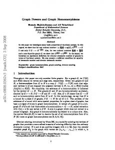
H r
G
r G
H G º H
Figure 1: The figure shows an example of the rooted product of G and H with a root r and illustrates the proof of Theorem 4. The green edges are edges in E1 . The blue edges (in the cycles) are edges in E2 . The red thick edges are edges in E3 . The graph G ◦ H consists of one copy of G and disjoint copies of H. Each copy of H − r are “far” enough that it needs a path of length at least 2 to traverse to another copy. color as E1 .) Again, this is a proper (partial) coloring because no edges of E1 ∪ E3 join endpoints of any two edges in E2 . So far, we have used χ0S (G) + χ0S (H − r) colors for E1 and E2 . Finally, we color E3 . Take a “vertex-coloring” σ3 : V (G) → [χ(G)] of G. We define from σ3 new degH (r) · χ(G) colors, denoted by (i, a) for i ∈ [χ(G)] and a : ra ∈ E(H). Then, for each edge (v, r)(v, a) ∈ E3 , we assign to (v, r)(v, a) a color σ((v, r)(v, a)) := (σ3 (v), a). So, the total number of colors we use in this step is χ(G) degH (r), thus suming up to χ(G) degH (r) + χ0S (G) + χ0S (H − r) colors as desired. It only remains to show that σ is a proper strong edge coloring of G ◦ H. To see this, consider a pair of edges (v, r)(v, a), (w, r)(w, b) ∈ E3 . We will check for any possible violation. If v = w, then (v, r) = (w, r), which means that the two edges receive different colors by construction, and we are done. Hence, we may assume that v 6= w. Now, (v, r)(v, a), (w, r)(w, b) share no endpoints. So, a possible violation is that some edge in E(G ◦ H) joins their endpoints. If (v, r)(v, a), (w, r)(w, b) are joined by an edge (v, r)(w, r) ∈ E1 , then we also have an edge vw ∈ E(G). So, σ3 (v) 6= σ3 (w), thus implying that (v, r)(v, a), (w, r)(w, b) receive different colors. Otherwise, (v, r)(v, a), (w, r)(w, b) are joined by an edge in E2 ∪ E3 . But, this is not possible since v 6= w whereas edges in E2 ∪ E3 are of the form (u, a)(u, b) where ab ∈ E(H). (Edges in E2 ∪ E3 only join vertices in the same copy of H.) Now, we prove the left-hand-side: max{χ0S (G), χ0S (H − r), degH (r) · χf (G)} ≤ χ0S (G ◦ H) . Clearly, max{χ0S (G), χ0S (H − r)} is the minimum number of colors that we need to strongly color edges of G ◦ H since G ◦ H has both G and H as subgraphs. So, it suffices to show that G ◦ H requires at least degH (r) · χf (G) colors. To prove this, we map a strong edge coloring of G ◦ H to a fractional vertex-coloring of G. Let C1 , C2 , . . . , CM be color classes of a minimum strong edge coloring in G ◦ H. We will show that χf (G) ≤ M/ degH (r). We define the fractional color classes of G by Di = {v ∈ V (G) : (v, r)(v, a) ∈ Ci for some a ∈ V (H)} for i = 1, 2, . . . , M . Then we assign a fractional value of 1/ degH (r) to each color class Di . Let us
7
check that these color classes form a proper fractional vertex-coloring of G, i.e., (1) each Di is a stable set in G and (2) each vertex belongs to at least degH (r) color classes. Suppose the first condition does not hold. Then there is an edge vw ∈ E(G) joining vertices u, v from the same color class Di . But, then there are edges (v, r)(v, a) and (w, r)(w, b) in the same (strong edge) color class Ci that are joined by an edge (v, r)(w, r), contradicting the fact that Ci forms an induced matching in G. Next, for the second condition, we know that each vertex (v, r) ∈ V (G ◦ H) has degH (r) neigbors of the form (v, a) where ra ∈ E(H). So, we have degH (r) edges in G ◦ H of the form (v, r)(v, a) where ra ∈ E(H), and these edges could not have the same colors (since they share (v, a) as an endpoint). It follows that v belongs to degH (r) color classes. This completes the proof. The statement of the above theorem can be simplified. Using the fact that χ(G) ≤ χf (G) log |V (G)| and choosing H as a star: Corollary 5. For any graph G and a star H with a root vertex r and ` leaves, ˜ 0S (G) + ` · χ(G)). χ0S (G ◦ H) = Θ(χ
3.1
Hardness
Our construction is simple. We take a graph G = (V, E) on N vertices which is a hard instance b = G ◦ H, which is the of the graph coloring problem as in Theorem 2, and we output a graph G 2 rooted product of G and a star H with ` = N leaves. See Figure 3.1. Now, we invoke Corollary 5 w2 w1
w3 v
G G
Figure 2: The figure shows an example of a reduction from an instance the graph coloring problem to the strong edge coloring problem with ` = 3. b ≤ N 2 N � + N 2 ≤ N 2+2� . In to analyze the hardness gap. In Yes-Instance, χ(G) ≤ N � implies χ0S (G) 2 N 1−� N 1−� 0 3−2� b ≥ b 1/3−� , No-Instance, χ(G) ≥ N implies χS (G) . So, the gap is N 1−� = |V (G)| log N ≥ N thus proving Theorem 1.
3.2
Distance-k Edge-Coloring
The hardness construction for the strong edge coloring problem can be generalized to distance-k b = G ◦ H as in the previous section. Then edge-coloring problem. For k = 3, we take an instance G we subdivide each edge (v, r)(w, r) of G ◦ H by a path of length 2, namely ((v, r), xvw , (w, r)). The 8
similar analysis as that of the case k = 2 gives a hardness of n1/3−� for this case. For k = 4, we change the choice of a graph H. Instead of using a star with N 2 leaves, we choose H as KN , a clique on N vertices. Then we apply the following lemma whose proof appears in Appendix B. Theorem 6. For any graph G and a clique K` , the following holds: � 2 � ` · χ(G) Ω ≤ χ(L4 (G ◦ K` )) ≤ O(`2 · χ(G) + |E(G)| + `|V (G)|). log |V (G)| To prove Theorem 6 we can use the same analysis as before except that now H is a clique KN . b is smaller while The advantage of using KN is that the number of vertices in the output graph G maintaining the same hardness gap. This approach allows us to prove the hardness of n1/2−� for the distance-k edge coloring. For k > 4, we modify the construction for k = 4 by replacing each edge uv of G by a path of length k − 3. For more detail, see Appendix B.
3.3
Strong Edge Coloring of Other Graph Products
We prove some bounds of the strong chromatic index of lexicographic (•) and disjunctive (∨) products of graphs which might be of independent interest. The proof here uses insights from that of Theorem 4. Roughly speaking, we show � ˜ |V (H)|2 χ0 (G) + χ(G)χ0 (H) χ0S (G • H) = Θ S S � ˜ |V (H)|2 χ0 (G) + |V (G)|2 χ0 (H) χ0S (G ∨ H) = Θ S S More precisely, we show the following theorems (see Appendix B). Theorem 7 (Lexicographic Product). For any graphs G and H, � � |V (H)|2 χ0S (G) χ(G)χ0S (H) max , ≤ χ0S (G • H) ≤ |V (H)|2 χ0S (G) + χ(G)χ0S (H) log |V (H)| log |V (G)| Theorem 8 (Disjunctive Product). For any graphs G and H, � � |V (H)|2 χ0S (G) |V (G)|2 χ0S (H) max , ≤ χ0S (G ∨ H) ≤ |V (H)|2 χ0S (G) + |V (G)|2 χ0S (H) log |V (H)| log |V (G)|
3.4
Other Bounds on Strong Edge Coloring
We also prove some bounds on the strong chromatic index of graphs. Precisely, we prove an upper bound on the strong chromatic index of a cograph, a graph that contains no path on four vertices as an induced subgraph, and we prove a lower bound on the chromatic index of a general graph. The proofs are provided in Appendix A.1 and A.2, respectively. Theorem 9. For any cograph G, χ0S (G) ≤ ∆2 (G). Moreover, if L2 (G) is not a complete graph then χ0S (G) ≤ ∆2 (G) − 1. Theorem 10. For any graph G, χ0S (G) ≥
δ(G)χf (G) . 2
9
4 4.1
Other Problems on Gk Vertex-Coloring and Maximum Clique
The graph coloring and maximum clique problems in Gk share the same behavior. Both problems admit approximation ratios of O(n1/2 ) when k ≥ 2 is even and O(n2/3 ) when k ≥ 3 is odd via greedy algorithms. (See Appendix C and D.) The hardness construction for these two problems are the same. We sketch a construction for the case k = 2 and defer the full proof for any k to Appendix. Given a graph G0 = (V 0 , E 0 ), we construct G by replacing each vertex v of degree d by star Sd+1 and then rewiring each edge to different vertex of Sd+1 . Note that Sd+1 is a tree on d + 1 vertices consisting of a root vertex r and d leaves. So, the root vertex r of Sd+1 corresponds to a vertex v of G0 . We call the root vertex of each star a canonical vertex. Moreover, two distinct canonical vertices r and r0 are within distance 2 of each other in G if and only if their corresponding vertices v and v 0 of G0 are adjacent. Thus, the chromatic (resp., clique) number restricted to canonical vertices corresponds to the chromatic (resp., clique) number of G0 . However, this number can be smaller than that restricted to non-canonical vertices. Hence, we make |V (G0 )| copies of each canonical vertex to ensure that the chromatic (resp., clique) number restricted to canonical vertices is larger than that of non-canonical vertices. So, we can derive the hardness of |V (G0 )|1−� from the graph coloring (resp., maximum clique) problem in G0 . Since the output graph G has |V (G)| = |V (G0 )|2 vertices, we have the hardness of n1/2−� -hardness, for any � > 0. For k > 2, we modify the construction by subdividing each edge uv corresponding to an edge of G by a path of length k − 1. So, the graph coloring and maximum clique problems in Gk admit no n1/2−� -approximation, for any � > 0, unless NP = ZPP.
4.2
Maximum Stable Set
We sketch tight hardness construction for the maximum stable set problem on Gk . For different k, the approximability of the problems varies, depending on the parity of k. Here we only discuss the case k = 2 and k = 3. The case of all odd and even k can be obtained by simply modifying these two constructions. We defer the full discussion to Appendix E. First, consider the case when k = 2. Let G be an input graph. The key idea is to subdivide each edge in E(G) so that each pair of non-adjacent vertices are in distance more than 2 of each other. Thus, any stable set in the graph has a corresponding stable set in its square. More formally, we construct a graph H by first subdividing each edge e ∈ E(G) by a special vertex x(e). To make sure that these special vertices would not form a stable set in H 2 , we add edges x(e)x(e0 ) for any pair of special vertices x(e), x(e0 ). Thus, α(G) ≤ α(H) ≤ α(G) + 1. As |V (H)| = |E(G)| + |V (G)| ≤ 2|V (G)|2 , we have an n1/2−� -hardness for computing α(G2 ). The hardness is √ tight because it matches the upper bounds of O( n)-approximation provided by the algorithm of Halld´orsson et al. [14]. For k = 3, the key idea of the construction is simply ensuring that any pair of vertices are not within distance 3 of each other. Given a graph G = (V, E) on n vertices, we construct a graph H by attaching a new vertex v ∗ to each vertex v ∈ V (G); we call v a white vertex and call v ∗ a black vertex. Now, we have a graph H on 2|V (G)| vertices. Observe that a pair of black vertices v ∗ and w∗ are in distance 3 of each other in H if and only if their corresponding white vertices v and w are adjacent in G. Thus, a set of black vertices S ∗ is stable in H 3 if and only if the set of white
10
vertices S = {v : v ∗ ∈ S ∗ } is stable in G. So, α(G) ≤ α(H 3 ) ≤ 2α(G). The |V (G)|1−� -hardness follows immediately.
References [1] Geir Agnarsson and Magn´ us M. Halld´orsson. Coloring powers of planar graphs. SIAM J. Discrete Math., 16(4):651–662, 2003. Also in SODA’00. 2 [2] Noga Alon and Bojan Mohar. The chromatic number of graph powers. Combinatorics, Probability & Computing, 11(1):1–10, 2002. 2 [3] Christopher L Barrett, Gabriel Istrate, Anil Kumar Vilikanti, Madhav Marathe, and Shripad V Thite. Approximation algorithms for distance-2 edge coloring. Technical report, Los Alamos National Lab., NM (US), 2002. 2 [4] Christopher L. Barrett, V. S. Anil Kumar, Madhav V. Marathe, Shripad Thite, and Gabriel Istrate. Strong edge coloring for channel assignment in wireless radio networks. In PerCom Workshops, pages 106–110, 2006. 1 [5] Parinya Chalermsook, Bundit Laekhanukit, and Danupon Nanongkai. Graph products revisited: Tight approximation hardness of induced matching, poset dimension and more. In SODA, pages 1557–1576, 2013. 3, 4, 14 [6] Miroslav Chleb´ık and Janka Chleb´ıkov´a. Complexity of approximating bounded variants of optimization problems. Theor. Comput. Sci., 354(3):320–338, 2006. Preliminary version in FCT 2003. 4 [7] Reinhard Diestel. Graph Theory. Graduate Texts in Mathematics, Volume 173. SpringerVerlag, Heidelberg, 4th edition, July 2010. 4, 22 [8] William Duckworth, David Manlove, and Michele Zito. On the approximability of the maximum induced matching problem. J. Discrete Algorithms, 3(1):79–91, 2005. 4 [9] Jeff Erickson, Shripad Thite, and David P. Bunde. Distance-2 edge coloring is NP-complete. CoRR, abs/cs/0509100, 2005. 2 [10] Ralph J. Faudree, Andr´ as Gy´ arf´ as, Richard H. Schelp, and Zsolt Tuza. Induced matchings in bipartite graphs. Discrete Math., 78(1-2):83–87, 1989. 2 [11] Ralph J. Faudree, Andr´ as Gy´ arf´ as, Richard H. Schelp, and Zsolt Tuza. The strong chromatic index of graphs. Ars. Combin., 29B:205–2011, 1990. 2 [12] Uriel Feige. Approximating maximum clique by removing subgraphs. SIAM J. Discrete Math., 18(2):219–225, 2004. 26 [13] Uriel Feige and Joe Kilian. Zero knowledge and the chromatic number. In CCC, pages 278–287, 1996. 3, 5 [14] Magn´ us M. Halld´ orsson, Jan Kratochv´ıl, and Jan Arne Telle. Independent sets with domination constraints. Discrete Appl. Math., 99(1-3):39–54, 2000. 10, 26 11
[15] Johan H˚ astad. Clique is hard to approximate within n1−� . In FOCS, pages 627–636, 1996. 5 [16] Herv´e Hocquard and Petru Valicov. Strong edge colouring of subcubic graphs. Discrete Appl. Math., 159(15):1650–1657, 2011. 2 [17] Ton Kloks, Sheung-Hung Poon, Chin-Ting Ung, and Yue-Li Wang. Algorithms for the strong chromatic index of Halin graphs, distance-hereditary graphs and maximal outerplanar graphs. In COCOON, pages 157–168, 2012. 2 [18] Daniel Kr´ al. Coloring powers of chordal graphs. SIAM J. Discrete Math., 18(3):451–461, 2004. 2 [19] Sven Oliver Krumke, Madhav V. Marathe, and S. S. Ravi. Models and approximation algorithms for channel assignment in radio networks. Wireless Networks, 7(6):575–584, 2001. 1 [20] Bundit Laekhanukit. Parameters of two-prover-one-round game and the hardness of connectivity problems. CoRR, abs/1212.0752, 2012. 2 [21] Yaw-Ling Lin and Steven Skiena. Algorithms for square roots of graphs. SIAM J. Discrete Math., 8(1):99–118, 1995. 22 [22] Errol L. Lloyd and Subramanian Ramanathan. On the complexity of distance-2 coloring. In ICCI, pages 71–74, 1992. 2 [23] Mohammad Mahdian. The strong chromatic index of graphs. Master’s thesis, University of Toronto, 2000. 2 [24] Mohammad Mahdian. On the computational complexity of strong edge coloring. Discrete Appl. Math., 118(3):239–248, 2002. 2 [25] S. McCormick. Optimal approximation of sparse hessians and its equivalence to a graph coloring problem. Math. Program., 26:153–171, 1983. 10.1007/BF02592052. 2, 22 [26] Michael S. O. Molloy and Bruce A. Reed. A bound on the strong chromatic index of a graph, . J. Comb. Theory, Ser. B, 69(2):103–109, 1997. 2 [27] Subramanian Ramanathan and Errol L. Lloyd. Scheduling algorithms for multihop radio networks. IEEE/ACM Trans. Netw., 1(2):166–177, 1993. Also in SIGCOMM’92. 1 [28] Mohammad R. Salavatipour. A polynomial time algorithm for strong edge coloring of partial k-trees. Discrete Appl. Math., 143(1-3):285–291, 2004. 2 [29] Olivier Togni. Strong chromatic index of products of graphs. Discrete Math. Theor. Comput. Sci., 9(1), 2007. 3, 14 [30] Michele Zito. Induced matchings in regular graphs and trees. In WG, pages 89–100, 1999. 4
12
A
Bounds on Strong Edge Coloring
In this section, we show some bounds on the strong chromatic index of a graph. First, we show the upper bound of the strong chromatic index of a cograph, a graph that has no path on 4 vertices, denoted by P4 , as an induced subgraph. Our upper bound of ∆2 (G) proves the conjecture of Erd¨ os and Neˇsetˇril for the class of cographs. This bound is tight as we have χ0S (G) = ∆2 (G) when G is a complete bipartite graph (which is also a cograph).
A.1
Strong Edge Coloring of Cographs
The next theorem shows the upper bound on the strong chromatic index of a cograph. Theorem 11. For any cograph G, ≤ χ0S (G) ≤ ∆2 (G). Moreover, if L2 (G) is not a complete graph then χ0S (G) ≤ ∆2 (G) − 1. Proof. To prove the theorem, it suffices to show that ∆(L2 (G)) ≤ ∆2 (G) − 1. Recall that ΓG (v) denotes the set of neighbors of a vertex v in a graph G. Consider an edge uv ∈ E(G), which is a vertex in L2 (G). We will count the number of neighbors at distance 2 of uv in L(G); that is, we calculate |ΓL2 (G) (uv)|. Clearly, the number of edges at distance 1 of uv in L(G) is 2∆(G) − 1. So, the trivial counting shows that ∆(L2 (G)) is at most 2(∆(G) − 1)(∆(G) − 1) + 2(∆(G) − 1) = 2(∆(G))(∆(G) − 1) We show that every edge at distance exactly 2 from uv is double counted in the trivial counting. To see this, we use a charging scheme. For each edge ab ∈ E(G) with no common endpoints with uv (i.e., {a, b}∩{u, w} = ∅), we charge ab by the cost function c(ab) = |{ua, ub, va, vb}∩E(G)|. That is, we count the number of edges that join ab to uv. We claim that c(ab) is either 0 or at least 2. If G has no edge joining ab to uv, then c(ab) = 0, and we are done. Suppose that G has an edge joining ab to uv. We may assume wlog that such edge is ua. Since G is P4 -free, G must have at least one edge from {ub, va, vb}. This implies that c(ab) ≥ 2. Hence, in the trivial counting, edges with distance 2 from u must have been double counted from the same side u (resp., v) or from both sides u and v. So, we conclude that 1 · 2(∆(G) − 1)(∆(G) − 1) + 2(∆(G) − 1) 2 ≤ (∆(G) − 1)(∆(G) − 1) + 2(∆(G) − 1)
∆(L2 (G)) ≤
= (∆(G) + 1)(∆(G) − 1) = ∆2 (G) − 1 Therefore, χ0S (G) = χ(L2 (G)) ≤ ∆(L2 (G)) + 1 = ∆2 (G), and by Brook’s Theorem, if L2 (G) is not a complete graph or an odd cycle, then χ0S (G) ≤ ∆2 (G) − 1. The statement can be straightened as we can rule out the case of an odd cycle. To be precise, a square of a graph could not be a cycle of length more than 3. (Note that an odd cycle of length 3 is exactly a complete graph K3 .) To see this, consider a graph H. It is easy to check that H 2 cannot form a cycle if H has no path of length 2 as a subgraph. So, assume that H has a path of length 2, namely (u, v, w). Then these vertices u, v, w must form a cycle in H 2 . So, H 2 is either a cycle of length 3 or contains it as a subgraph, which means that H 2 cannot be a cycle of length more than 3. This proves the theorem. 13
A.2
Lower Bound on Strong Edge Coloring of General Graphs
A lower bound slightly better than a trivial bound of ∆(G) for the strong chromatic index of a general graph is shown in the next theorem. The proof is based on a simple fractional coloring argument. Theorem 12. For any graph G, χ0S (G) ≥
δ(G)χf (G) , 2
where δ(G) is the minimum degree of G.
Proof. If δ(G) = 0, then the statement is trivial. So, we assume that δ(G) > 0. We first number vertices of G by 1, 2, . . . , |V (G)|, and we think of each vertex v as an integer. Now, take a minimum strong edge coloring σ of G. We will construct from σ a list of colors L(v) for each vertex v of G. For each edge vw incident to v, we add to L(v) a color (σ(vw), 1) if v > w and a color (σ(vw), 2) otherwise. So, we have used at most 2χ0S (G) colors, and each vertex v has a list L(v) of degG (v) colors. We claim that, for any adjacent vertices v and w, L(v) ∩ L(w) = ∅. To see this, first, all edges incident to vw have different colors by the definition of strong edge coloring: For an edge vw, vertices v and w must pick different colors from vw, namely (σ(vw), 1) and (σ(vw), 2) by construction. So, v and w cannot have the same color in their lists. Thus, we may think of these color-lists as a fractional coloring of G in which we pick each color with a fraction 1/δ(G). It can be seen that this is a proper fractional coloring of G since each vertex has at least δ(G) colors in its list. Therefore, χf (G) ≤ 2χ0S (G)/δ(G), proving the theorem.
A.3
Strong Edge Coloring of Graph Products
The strong edge coloring problem has a close connection with the maximum induced matching problem, which asks for the maximum size of an induced matching in a graph. The tight hardness of approximation of the latter problem in a bipartite graph was recently proved by Chalermsook et al. in [5] by a graph product technique. So, studying the properties of the chromatic index of graph products might shed some light on proving a stronger hardness result of the strong edge coloring problem. Strong edge coloring of graph products has also been studied by Togni [29]. Here we prove graph product inequalities in the cases not considered by Togni, so our work completes the story of graph products w.r.t. strong chromatic index. Theorem 13 (Lexicographic Product). For any graphs G and H, � � |V (H)|2 χ0S (G) χ(G)χ0S (H) max , ≤ χ0S (G • H) ≤ |V (H)|2 χ0S (G) + χ(G)χ0S (H) log |V (G)| log |V (G)| Proof. Before proceeding, we outline the proof. The lower bound is proved by projecting the strong edge coloring of the lexicographic product of G and H to the coloring in the original graphs. However, as we have more colors in the graph product, we map the coloring back to the original graphs as the fractional coloring. The upper bound is proved by simply projecting the strong edge coloring of G and H to their lexicographic product. As we have multiple copies of G and H in the graph product, we put different sets of colors for each copy and thus have the bound as in the statement of the theorem. Lower Bound:
14
We partition the edges in E(G • H) into E(G • H) = EG ∪ EH , where EG = {(u, i)(v, j) : uv ∈ E(G)} EH = {(u, i)(u, j) : u ∈ V (G), ij ∈ E(H)} The proof of this part is done in the following two claims. Claim 14. |V (H)|2 χ0S (G) log |V (G)| ≤ χ0S (G • H). Proof. To prove this claim, it is sufficient to show that χf (L2 (G)) ≤ χ0S (G • H)/|V (H)|2 , since it would then imply: |V (H)|2 χ0S (G) χ0S (G • H) ≥ log |V (G)| (because fractional coloring and coloring are within logarithmic factor of each other). And we show this by giving a fractional coloring of L2 (G) using a strong edge coloring of G • H. For each vertex u ∈ V (G), define Vu = {(u, a) : a ∈ V (H)}. Then, for any edge uw of G, the subgraph G • H[Vu ∪ Vw ] forms a complete bipartite graph with |V (H)|2 edges. So, edges of G • H[Vu ∪ Vw ] must all have different colors in any proper strong edge coloring of G • H. Now, we take any strong edge coloring of G•H and will use it to define a (fractional) strong edge coloring of graph G. For each edge uw ∈ E(G), we pick one edge (u, a)(w, b) from G•H[Vu ∪Vw ] and color the edge uw of G by the color of (u, a)(w, b). Observe that this is a proper strong edge coloring of G. Suppose not. Then we must have an edge uw and xy that are in distance two and have the same color. We may assume that G has an edge ux, the color of uw is taken from (u, a)(w, b) and the color of xy is taken from (x, c)(y, d). But, then we would have an edge (u, a)(x, c) in G • H, implying that (u, a)(w, b) and (x, c)(y, d) must have different colors, a contradiction. Thus, we may think of the strong edge coloring of G • H on EG as a fractional coloring of G in which we choose each color class with fraction 1/|V (H)2 |. This means that we only use χ0S (G • H)/|V (H)|2 fractional colors. Claim 15. χ(G)χ0S (H)/ log |V (G)| ≤ χ0S (G • H). Proof. We prove the claim by showing a fractional vertex coloring of G using χ0S (G • H)/χ0S (H) fractional colors. This would imply that: χ0S (G • H) ≥
χ(G)χ0S (H) log |V (G)|
Take any strong edge coloring of G • H, and consider colors of the edge set EH = {(u, i)(u, j) : u ∈ V (G), ij ∈ E(H)}. Define Vu = {(u, i) : u ∈ V (G), i ∈ V (H)}. Observe that G • H[Vu ] is isomorphic to H. So, any strong edge coloring of G•H on E(G•H[Vu ]) induces a proper strong edge coloring of H. Moreover, any edge (u, i)(x, a) ∈ Vu and any edge (w, j)(y, b) ∈ Vw have different colors if and only if G has an edge uw because G • H[Vu ∪ Vw ] forms a complete bipartite graph. So, if we color each vertex u of G by the color of some edge (u, i)(x, a) in G • H, then we have a valid vertex-coloring of G. We think of coloring of edges in E(G • H[Vu ]) as a fractional coloring of vertices in G, where we pick each color with a fraction 1/χ0S (H); this is a proper fractional vertex-coloring of G because edges of E(G • H[Vu ]) must have at least χ0S (H) colors.
15
Upper Bound: We partition the edges in E(G • H) into E(G • H) = EG ∪ EH where EG = {(u, i)(v, j) : uv ∈ E(G)} EH = {(u, i)(u, j) : u ∈ V (G), ij ∈ E(H)} We argue that the number of colors needed to color EG and EH is |V (H)|2 χ0S (G) and χ(G)χ0S (H) respectively. The second inequality is proved as follows. Let C1 , . . . , Cχ(G) be color classes of G. x } where E x = {(u, i)(u, j) : u ∈ C , ij ∈ E(H)}. Each E x can be colored Partition EH into {EH x x H H 0 by at most χS (H) colors. ˜1 , . . . , E ˜g be the strong coloring of edges The first inequality is a bit more complicated. Let E Sg g0 g in E(G) = g0 =1 Eg0 . We further partition EG by strong-coloring classes into {EG }g0 =1 where g0 ˜g0 }, which can be further partitioned by the two endpoints of H. EG = {(u, i)(v, j) ∈ EG : uv ∈ E That is, [ g0 g0 = EG (i, j) EG i,j∈V (H) g0
˜g0 }. It is now easy to check that each of these sets is an where EG (i, j) = {(u, i)(v, j) : uv ∈ E induced matching, so only one color is needed for each of them. Theorem 16 (Disjunctive Product). For any graphs G and H, � � |V (H)|2 χ0S (G) |V (G)|2 χ0S (H) max , ≤ χ0S (G ∨ H) ≤ |V (H)|2 χ0S (G) + |V (G)|2 χ0S (H) log |V (G)| log |V (H)| Sketch. The proof is similar to the case of the lexicographic product. That is, we project the strong edge coloring of G∨H into G and H to obtain the lower bound and project the strong edge coloring of G and H into G ∨ H to obtain the upper bound. The difference in the analysis is that when we partition edges of G ∨ H into EG and EH , the two set are symmetric. To be precise, EG = {(u, i)(v, j) : uv ∈ E(G)} EH = {(u, i)(v, j) : ij ∈ E(H)} The set EG is in fact that same as that in the proof of the lexicographic product. Thus, we can apply the same analysis and obtain the similar bounds, which are symmetric in this case.
B
Distance-k Edge-Coloring
The distance-k edge-coloring is a generalization of the strong edge coloring where any two edges of distance at most k receive different colors. So, the distance-k edge-coloring of G is equivalent to the vertex-coloring of Lk (G).
B.1
Hardness
We show the approximation hardness of n1/3−� for the case k = 3 and n1/2−� for the case k ≥ 4. Our constructions are different for the case k = 3 and k ≥ 4. But, both cases follow the idea that we use in proving the hardness of the strong edge coloring problem. 16
B.2
The Case k = 3
We start from the hardness construction of the strong edge coloring problem as in Section 3. Recall b is the rooted product G b = G ◦ S`+1 of a graph G = (V, E) and a star S`+1 , where that the graph G G = (V, E) is a graph on N vertices which is a hard instance of the graph coloring problem as in b can be thought of as a graph obtained Theorem 2, and S`+1 is a star with ` leaves. (In fact, G b a graph G from G by adding ` edges hanging from each vertex v ∈ V (G).) We construct from G by subdividing each edge vw ∈ E(G) by a path of length two, namely, ((v, r), xuv , (w, r))). We call b (a copy of v ∈ V (G)) the ` edges (v, r)(v, a), where ra ∈ S`+1 , hanging from each vertex (v, r) of G canonical edges, and we call other edges non-canonical edges. Observe that G has `|V (G)| canonical edges and 2|E(G)| non-canonical edges. The following claim shows a relation between edges in G and edges in L3 (G)). Claim 17. For any two distinct vertices v and w in G, canonical edges (v, r)(v, a) and (w, r)(w, b), for any ra, rb ∈ E(S`+1 ), are adjacent in L3 (G) if and only if v and w are adjacent in G. Proof. First, if v and w are adjacent in G, then by construction, we have a path ((v, r), xvw , (w, r)) in G. This means that (v, r)(v, a) and (w, r)(w, b) are adjacent in L3 (G). Conversely, suppose e = (v, r)(v, a) and f = (w, r)(w, b) are adjacent in L3 (G). Then we have a path P of length either 1, 2 or 3 connecting e and f in L3 (G). Note that any path P from e to f has to visit both (v, r) and (w, r) (which are edges in L(G)). So, if P is a path of length 1, then we must have (v, r) = (w, r) (i.e., v = w), which is not possible. If P is a path of length 2, then P cannot visit any other vertex of G except (v, r) and (w, r). But, again, this is not possible since, by construction, the only way to go from (v, r) to (w, r) is to visit a vertex xuy , for some edge uy ∈ E(G) (xuy is a subdividing vertex). Thus, P must be a path of length 3. Since P has to visit (v, r) and (v, w), the only way for P to be a path of length 3 in L(G) is to use a vertex xvw . Hence, v and w are adjacent in G. This completes the proof. The next lemma shows a connection between χ(G) and χ(L3 (G)). The proof is similar to the proof of Theorem 4. As we only need to prove the hardness result, we use some trivial bounds to make the proof simpler. Lemma 18. ` · χf (G) ≤ χ(L3 (G)) ≤ ` · χ(G) + 2|E(G)|. Proof. First, we prove the upper bound. We color non-canonical edges by different colors. So, we have a partial coloring σ that uses 2|E(G)| colors, and it is trivial that σ is a proper (partial) distance-3 edge-coloring of G. Next, we color canonical edges using a minimum vertex-coloring of G, namely σ 0 : V (G) → [χ(G)]. Precisely, we color each canonical edge e = (v, r)(v, a) by a color σ(e) = (σ 0 (v), ra). So, canonical edges having the same endpoint (v, r) receive different colors. For any two canonical edges, (v, r)(v, a) and (w, r)(w, b), they can receive the same color only if σ 0 (v) = σ 0 (w) and a = b. Since σ 0 is a proper vertex-coloring of G, vertices v and w can receive the same color only if v and w are not adjacent in G. So, by Claim 17, we conclude that σ((v, r)(v, a)) = σ((w, r)(w, b)) only if (v, r)(v, a) and (w, r)(w, b) are not adjacent in L3 (G). This shows that σ is a proper distance-3 edge-coloring of G, proving the upper bound. Now, we prove the lower bound by defining from a minimum distance-3 edge-coloring σ : E(G) → [χ(L4 (G))] of G a fractionally (vertex) coloring of G. We define sets of vertices, which we claim to be (vertex) color classes of G, namely C1 , C2 , . . . , Cχ(L4 (G)) , where Ci = {v ∈ V (G) : σ((v, r)(v, a)) = i for some ra ∈ E(S`+1 )} 17
Then we assign a fractional value 1/` to each color class Ci . It can be seen that this gives a fractional (vertex) coloring of G with a weight of χ(L4 (G))/`. So, we are left to verify that this is a proper fractional coloring, i.e., (1) each Ci is a stable set in G and (2) each vertex is contained in at least ` color classes. The second condition is easy since we know that canonical edges sharing the same endpoint (v, r) could not receive the same color, and we have ` canonical edges (v, r)(v, a) incident to (v, r). To see that Ci is a stable set in G, consider a pair of canonical edges (v, r)(v, a) and (w, r)(w, b) in E(G) that receive the same color i. So, (v, r)(v, a) and (w, r)(w, b) are not adjacent in L3 (G). By Claim 17, we have that v and w are not adjacent in G. Thus, Ci forms a stable set in G. Therefore, χf (G) ≤ χ(L4 (G))/` =⇒ ` · χf (G) ≤ χ(L4 (G))
Hardness: Now, we take ` = N 2 and thus have a graph G on O(N 3 ) vertices. Recall that χ(G) ≤ χf (G) log |V (G)|. So, by invoking Lemma 18, we have • Yes-Instance: α(G) ≤ N � =⇒ χ(L4 (G)) ≤ ` · N � + 2|E(G)| ≤ N 2+2� . • No-Instance: α(G) ≥ N 1−� =⇒ χ(L4 (G)) ≥ ` · N 1−� / log N ≥ N 3−2� . Therefore, Theorem 2 implies that it is hard to approximate the distance-3 edge-coloring problem to within a factor of |V (G)|1/3−ε unless NP = ZPP.
B.3
The case k = 4
The hardness for the case k = 4 is similar to the case k = 2 (which is the strong edge coloring). We first prove general bounds on the distance-4 edge-coloring of the rooted product of graphs G and H. In particular, we prove the following theorem, which will play a role in proving the hardness of approximating distance-4 edge-coloring problem. Our proof is similar to the proof for the case of strong edge coloring. Theorem 19. For any graph G and a clique K` rooted r ∈ V (K` ), the following holds: Ω(max{χ(L4 (G)), `2 · χf (G), ` · χf (G3 )}) ≤ χ(L4 (G ◦ K` )) ≤ O(χ(L4 (G)) + `2 · χ(G) + ` · χ(G3 )) Proof. First, we partition edges of G ◦ K` into three parts, i.e., E(G ◦ K` ) = E1 ∪ E2 ∪ E3 , where E1 = {(v, r)(w, r) : vw ∈ E(G)}, [ E2 = {(v, a)(v, b) : a, b 6= r, ab ∈ E(G)}, v∈V (G)
E3 = E(G ◦ K` ) − (E1 ∪ E2 ) = {(v, r)(v, a) : ra ∈ E(K` )} Observe that E1 is a copy of edges of a G in G ◦ K` , E2 consists of copies of E(K` − r) = E(K`−1 ), and E3 is the set of other edges. It can be seen that there is a mapping between a coloring on E1 and a coloring on E(G). So, our technical part is to color E2 and E3 . Our proof has two parts. In the first part, we map (vertex) coloring on G, G3 , L4 (G) to edges of G ◦ K` . In the second part, we map a distance-4 edge-coloring on G ◦ K` to G and G3 . For this task, we argue through a fractional 18
coloring argument, i.e., we map the distance-4 edge-coloring on G ◦ K` to fractional colorings on G and G3 . Now, we prove the upper bound: χ(L4 (G ◦ K` )) ≤ O(χ(L4 (G)) + `2 · χ(G) + ` · χ(G3 )) First, take a distance-4 edge-coloring σ1 : E(G) → [χ(L4 (G))] of G. We color each edge (v, r)(w, r) ∈ E1 by a color σ((v, r)(w, r)) = σ1 (vw). This must be a proper (partial) distance 4-edge coloring of G ◦ K` because no edges of E2 and E3 join endpoints of edges in E1 . So, we are now using |χ(L4 (G))| colors. Second, take a vertex coloring σ2 : V (G) → [χ((G))] of G. We color each edge (v, a)(v, b) ∈ E2 by a color σ((v, a)(v, b)) = (σ2 (v), ab). We claim that this is a proper (partial) distance 4-edge coloring of G ◦ K` . Suppose not. Then there is a pair of edges (v, a)(v, b) and (w, a)(w, b) in E2 , where v 6= w, that receive the same color (c, ab), but their endpoints are connected by a path P on at most 4 vertices. So, v and w receive the same color c from σ1 . By the definition of G ◦ K` , P must be of the form (v, x)(v, r)(w, r)(w, y), where x, y ∈ {a, b}, because any path from (v, x) to (w, y) has to visit (v, r) and (w, r). But, this would mean that v and w are adjacent in G, which is a contradiction since v and w receive the same color. Now, we are using |χ(L4 (G))| + O(`2 · χ(G)) colors. Third, take a vertex coloring σ3 : V (G) → [χ((G3 ))] of G3 . We color each edge (v, r)(v, a) ∈ E3 by a color σ((v, r)(v, a)) = (σ2 (v), ra). We claim that this is a proper distance-4 edge-coloring of G ◦ K` . (It is obvious that the last set of colors are different from the previous sets.) So, it suffices to verify that no edges in E3 whose endpoints are connected by a path on at most 4 vertices receive the same color. Suppose not. Then there is a pair of edges (v, r)(v, a) and (w, r)(w, a) in E3 that receive the same color (c, ra), but their endpoints are connected by a path P on at most 4 vertices. By the definition of G ◦ K` , any path from (v, a) to (w, a) must visit (v, r) and (w, r). So, P must be of the form ((v, r), . . . , (w, r)), and each vertex in P must be of the form (u, r), where u ∈ V (G). That is, P is a copy of a path of G in G ◦ K` . But, this would mean that P is a v, w-path of length 3, which is a contradiction since v and w receive the same color in G3 . Therefore, we have a proper distance-4 edge-coloring of G ◦ K` with O(`2 · χ(G)) + χ(L4 (G)) + ` · χ(G3 ), proving the upper bound. Next, we prove the lower bound: Ω(max{χ(L4 (G)), `2 · χf (G), ` · χf (G3 )}) ≤ χ(L4 (G ◦ K` )) It is easy to see that we need at least χ(L4 (G)) colors to color G ◦ K` since G ◦ K` contains a copy of G. It remains to prove the second and last terms in the bound. We will show that we need at least Ω(`2 · χf (G)) colors to color edges of G ◦ K` . To see this, take a proper distance-4 edge-coloring σ : V (L(G ◦ K` )) → [χ(L4 (G ◦ K` ))] of G ◦ K` . Then we define a (vertex) color classes C1 , . . . , Cp of G from a coloring on E2 as Ci = {v ∈ V (G) : σ((v, a)(v, b)) = i for some a, b 6= r}, and we assign a fractional value of 1/|E(K `−1 )| = 1/Θ(`2 ) to each color class Ci . So, the total weight of this fractional coloring is χ(L4 (G ◦ K` ))/Θ(`2 ). Let us check that this is a proper fractional coloring of G. That is, we have to verify that (1) each Ci is a stable set in G, and (2) each vertex v ∈ V (G) is contained in at least |E(K` − r)| color classes. The latter is trivial since the set of vertices U = {(v, a) : a ∈ K` − r} forms a clique in G ◦ K` . (In fact, (G ◦ K` )[U ] is a copy of K` − r.) This means that v is contained in |E(K` − r)| color classes. It remains to verify that Ci is stable in G. Suppose not. Then there is a color class Ci containing two vertices v and w that are adjacent in G. By the construction of Ci , we must also have a pair of edges (v, a)(v, b) and (w, x)(w, y) in G ◦ K` , where a, b, x, y 6= r, that receive the same color i from σ. 19
But, this is not possible because vw ∈ E(G) implies that G ◦ K` have a path (v, a)(v, r)(w, r)(w, x) on 4 vertices connecting endpoints of (v, a)(v, b) and (w, x)(w, y), contradicting the fact that σ is a proper distance-4 edge-coloring of G. Thus, χ(G ◦ K` )/Θ(`2 ) ≥ χf (G) =⇒ χ(G ◦ K` ) ≥ Ω(`2 · χf (G)) Finally, we show that we need at least Ω(` · χf (G3 )) colors to color edges of G ◦ K` . Again, we take a proper distance-4 edge-coloring σ : V (L(G ◦ K` )) → [χ(L4 (G ◦ K` ))] of G ◦ K` . Then we define a (vertex) color classes C1 , . . . , Cp of G3 from a coloring on E3 as Ci = {v ∈ V (G) : σ((v, r)(v, a)) = i for some a 6= r}, and we assign a fractional value of 1/` to each color class Ci . So, the total weight of this fractional coloring is χ(L4 (G ◦ K` ))/(` − 1). Let us check that this is a proper fractional coloring of G3 . That is, we have to verify that (1) each Ci is a stable set in G, and (2) each vertex v ∈ V (G) is contained in at least ` color classes. The latter is trivial since there are (` − 1) edges in G ◦ K` with (v, r) as an endpoint. (In fact, these edges are of the form (v, r)(v, a) where a ∈ V (K` − r).) This means that v is contained in (` − 1) color classes. It remains to verify that Ci is stable in G3 . Suppose not. Then there is a color class Ci that contains two vertices v, w ∈ V (G) connected by a path of length 3 in G, namely P = (v, u, y, w). By the construction of Ci , we must also have a pair of edges (v, r)(v, a) and (w, r)(w, b) in G ◦ K` , where a, b 6= r, that receive the same color i from σ. But, this is not possible because, otherwise, G ◦ K` would have a path (v, r)(u, r)(y, r)(w, r) on 4 vertices connecting endpoints of (v, r)(v, a) and (w, r)(w, b), which contradicts the fact that σ is a proper distance-4 edge-coloring of G. Thus, χ(G ◦ K` )/(` − 1) ≥ χf (G3 ) =⇒ χ(G ◦ K` ) ≥ Ω((` − 1) · χf (G3 )) This completes the proof. The simplified version of Theorem 19 is as follows. (The Corollary appears as Theorem 6 in the main paper.) Corollary 20. For any graph G and a clique K` rooted r ∈ V (K` ), the following holds: � 2 � ` · χ(G) Ω ≤ χ(L4 (G ◦ K` )) ≤ O(`2 · χ(G) + |E(G)| + `|V (G)|). log |V (G)| Hardness: Take a graph G = (V, E) on N vertices, which is a hard instance of the graph coloring b of the distance-4 edge-coloring problem by problem as in Theorem 2. We construct a graph G taking the rooted product of G and a clique K` rooted at a vertex r ∈ V (K` ), where ` = N . So, b = G ◦ KN , and G b has O(N 2 ) vertices. Now, we apply Corollary 20 and have G • Yes-Instance: α(G) ≤ N � =⇒ χ(L4 (G)) ≤ O(`2 N � + |E(G)| + ` · N ) ≤ N 2+2� • No-Instance: α(G) ≥ N 1−� =⇒ χ(L4 (G)) ≥ Ω(`2 N 1−� / log N ) ≥ N 3−2� Therefore, Theorem 2 implies that it is hard to approximate the distance-3 edge-coloring problem to within a factor of |V (G)|1/3−ε unless NP = ZPP.
20
B.4
The case k > 4
The construction for the case k > 4 is based on that of the case k = 4. We apply a similar reduction as we have done in transforming the hard instance of the case k = 2 to that of the case k = 3. Specifb = G ◦ KN that we construct in the case k = 4. Then we subdivide each ically, we take a graph G edge ((v, r)(w, r)) of G ◦ KN by a path on k − 2 vertices, namely ((v, r), x1,vw , . . . , xk−4,vw , (w, r)). This results in a graph G. We call edges of the form (v, a)(v, b) where a, b 6= r and ab ∈ E(KN ) canonical edges and call other edges non-canonical edges. So, G has Θ(N 3 ) canonical edges and O(N 2 ) non-canonical edges. Then we can prove the next claim by the same arguments as used in Claim 17. We provide the proof only for the sake of completeness. Readers may skip the proof of the claim. Claim 21. For any two distinct vertices v and w in G, a pair of canonical edges (v, a)(v, b) and (w, c)(w, d) (i.e., ab, cd ∈ E(K` ) and a, b, c, d 6= r) are adjacent in Lk (G) if and only if v and w are adjacent in G. Proof. First, if v and w are adjacent in G, then by construction, we have a path ((v, r), x1,vw , . . . , xk−4,vw , (w, r)) in G. This means that (v, r)(v, a) and (w, r)(w, b) are adjacent in Lk (G). Conversely, suppose e = (v, r)(v, a) and f = (w, r)(w, b) are adjacent in Lk (G). Then we have a path P of either length 1, length between 2 and k − 1 or length k connecting e and f in Lk (G). Notice that any path P from e to f has to visit both (v, r) and (w, r). So, if P is a path of length 1, then we must have (v, r) = (w, r) (i.e., v = w), which is not possible. The case that P has length between 2 and k − 1 is also not possible. To see this, first, by construction, any path P between (v, r) and (w, r) in L(G) must visit at least k vertices (since we replace each edge (v, r)(w, r) of b by a path on k − 2 vertices). So, P has length at least k in L(G). The only way that P could G have length k is that P visits exactly k − 4 vertices of the form xi,uy . In fact, we may assert that uy = vw. Thus, vw must be adjacent in G. This completes the proof. The following corollary can be deduced from Claim 21 and the proof of Theorem 19. The proof resemblances that of Theorem 19. Corollary 22. Ω(N 2 · χf (G)) ≤ χ(Lk (G)) ≤ O(N 2 · χ(G)). Proof. For the upper bound, we color non-canonical edges by different colors. So, we use O(N 2 ) colors on these edges. Then we color each canonical edge using a minimum vertex-coloring σ of G. Precisely, we color each canonical edge (v, a)(v, b) by a color (σ(v), ab). So, edges e = (v, a)(v, b) and f = (w, c)(w, d) receive different colors if v = w or {a, b} = 6 {c, d}. If v 6= w and {a, b} = {c, d}, then e and f can receive the same color only if vw ∈ / E(G). So, Claim 22 implies that ef ∈ / E(Lk (G)). Thus, we have a proper distance-k edge-coloring of G. Now, we have used O(N 2 · χ(G)) colors, thus implying the upper bound. For the lower bound, we map a minimum distance-k edge-coloring σ 0 on canonical edges of G to a fractional coloring of G. In particular, we define color classes Ci = {v ∈ V (G) : σ 0 ((v, a)(v, b)) = i}. Then we assign a weight of 2/(N − 1)(N − 2) to each color class. Each Ci is a stable set because edges e = (v, a)(v, b) and f = (w, c)(w, d) could receive the same color only if ef ∈ / k E(L (G)), and Claim 21 implies that, in this case, vw ∈ / E(G). It is easy to see that there are (N − 1)(N − 2)/2 canonical edges (v, a)(v, b) for each vertex v ∈ V (G). Thus, the coloring we define is a proper fractional coloring of G. Now, the total weight is O(χ(Lk (G))/N 2 ). Therefore, χ(Lk (G)) ≥ Ω(N 2 χf (G)). 21
Hardness: Now, we invoke Corollary 22 to analyze the hardness gap. Recall that χ(G) ≤ χf (G) log |V (G)|. So, we have • Yes-Instance: α(G) ≤ N � =⇒ χ(Lk (G)) ≤ O(N 2 · N � ) ≤ N 2+2� . • No-Instance: α(G) ≥ N 1−� =⇒ χ(Lk (G)) ≥ Ω(N 2 · N 1−� / log N ≥ N 3−2� . The graph G has O(k|E(G)|+`2 |V (G)|) = O(N 2 ) (since ` = N and k is a constant). So, the gap between χ(Lk (G)) in Yes − Instance and No − Instance is |V (G)|1−ε Thus, Theorem 2 implies that it is hard to approximate the distance-3 edge-coloring problem to within a factor of |V (G)|1/2−ε unless NP = ZPP.
C
Graph Coloring
In this section, we consider the problem of coloring the k-th power of a graph. The complexity of the problem of coloring the k-th power of a graph is known to be NP-hard [25, 21]. For k = 2, the problem of coloring the square of a graph, McCormick [25] showed that a greedy coloring algorithm √ gives O( n)-approximation. Generalizing the analysis of McCormick, we show that the greedy √ coloring algorithm yields an O( n)-approximation, for all k ≥ 2 when k is even and O(n2/3 )approximation for all k ≥ 3 when k is odd. Moreover, we show that this bound is tight for any even constant k; that is, the problem does not admit an n1/2−� -approximation algorithm for any � > 0 unless NP = ZPP.
C.1
Algorithm
The algorithm is a greedy coloring algorithm, which processes vertices in some order and, when processing a vertex v, colors v by a color i that is the smallest color number that has not been used before by v’s neighbors. It is known by Brooks’ theorem that the greedy coloring algorithm uses at most ∆(G) colors unless G is a complete graph or an odd cycle; for the latter two cases, it uses at most ∆(G) + 1 colors. See [7] for more detail. It remains to analyze the performance guarantee of the algorithm. Before proceeding, we need to prove some simple facts. Let Γ(v, k) denote the set of vertices that are within distance k from v, and define f (k) = max{|Γ(v, k))| : v ∈ V (G)}. The function f (k) in fact denotes the maximum degree of vertices in Gk . Proposition 23. For any k ≥ 2, the following holds • The set of vertices Γ(v, bk/2c) ∪ {v} induces a clique in Gk . � f (bk/2c)2 if k is even • f (k) ≤ f (bk/2c)f (dk/2e) ≤ f (bk/2c)2 ∆(G) if k is odd Proof. The first statement follows because any pair of vertices in the set Γ(v, bk/2c)∪{v} are within distance two of each other in Gbk/2c , so they become immediate neighbors in Gk . Now, we prove the second statement. For any vertex v, there are at most f (bk/2c) vertices in distance at most bk/2c from v by definition, and each of them has at most f (dk/2e) vertices within distance at most dk/2e. If k is even dk/2e = bk/2c. So, the number of vertices in distance 2bk/2c from v is at most f (bk/2c)2 , proving the case when k is even. For the case that k is odd, each vertex within distance dk/2e − 1 = bk/2c from v ∈ V has at most ∆(G) neighbors. Thus, f (dk/2e) ≤ f (bk/2c)∆(G), proving the case that k is odd. 22
The above proposition implies the following. Proposition 24. f (bk/2c) ≤ χ(Gk ) ≤ f (bk/2c)f (dk/2e) Proof. The first inequality follows since Gk has a clique of size at least f (bk/2c) by the first statement of Proposition 23. The second inequality follows since Gk has maximum degree at most f (bk/2c)f (dk/2e) by the second statement of Proposition 23, and the greedy algorithm gives a coloring with at most ∆(Gk ) = f (k) colors. The following corollary is now immediate. Corollary 25. The greedy coloring is an f (bk/2c) approximation when k is even and ∆(G)f (bk/2c) approximation when k is odd. C.1.1
Analysis of The Greedy Algorithm.
Now, we analyze the performance guarantee of the greedy algorithm. Recall that the greedy algorithm gives a coloring with at most ∆(Gk ) = f (k) colors. √ √ Case 1: k is even. If f (bk/2c) ≥ n, then χ(Gk ) ≥ n by Proposition 24. So, any algorithm √ √ gives an O( n)-approximation since χ(G) ≤ n. Otherwise, if f (bk/2c) < n, then the greedy √ algorithm yields an approximation ratio of f (bk/2c) < n by Corollary 25. Case 2: k is odd. If f (bk/2c) ≥ n1/3 , then χ(Gk ) ≥ n1/3 by Proposition 24. So, any algorithm gives an O(n2/3 )-approximation since χ(G) ≤ n. Otherwise, if f (bk/2c) < n2/3 , then the greedy algorithm yields an approximation ratio of f (bk/2c)∆(G) ≤ f (bk/2c)2 < n2/3 by Corollary 25. Note that the approximation ratio is tight for any algorithm that gives O(∆(G))-approximate coloring. We show this by constructing an example of graph G where ∆(G3 )/χ(G3 ) = Ω(|V (G)|2/3 ). The graph G is a full d-ary tree with height 4. (A full d-ary tree is a tree where each non-leaf vertex has exactly d neighbors.) Notice that ∆(G3 ) = d3 + d2 because every vertex has a path of length 3 from a root vertex while χ(G)3 = 3d + 1.
C.2
Hardness
In this section, we show an application of a “fractional coloring” argument used in Section 3 in proving hardness of approximations for coloring of the k-th power of a graph stated formally as below. Theorem 26. For any � > 0, unless NP = ZPP, it is hard to distinguish the following two cases of a given graph G on n vertices. • Yes-Instance: χ(Gk ) ≤ n� . • No-Instance: χ(Gk ) ≥ n1/2−� . In particular, it is hard to approximate the chromatic number of a graph to within a factor of n1/2−� , for all � > 0, unless NP = ZPP. Our result is derived from the hardness of the graph coloring problem as in Theorem 2. 23
Construction. The construction is as follows. Let ` be a parameter. Take a graph G = (V, E) on n vertices, which is a hard instance of the graph coloring problem as in Theorem 2. We construct a graph G0 = (X ∪ Y, E 0 ) as follows. First, for each edge vw ∈ E, we construct a path (x(vw, 1), . . . , x(vw, k − 1)) We remark that x(vw, i) = x(wv, k − S i), for all edges vw ∈ E(G). (They are just indexed from different directions.) Denote by X = vw∈E(G) {x(vw, i) : i ∈ [k − 1]}. For each vertex v ∈ V , we create ` vertices {y(v, 1), . . . , y(v, `)} and add an edge joining each vertexSy(v, j) to all the vertices in X of the form x(vw, 1) for all w : vw ∈ E(G). Denote by Y = v∈V (G) {y(v, j) : j ∈ [`]}. Choosing ` = n, the number of vertices of G0 = (X ∪ Y, E 0 ) is at most |X| + |Y | ≤ `|V (G)| + (k − 1)|E(G)| = O(n2 ) since k is a constant. This completes the construction. The reduction is illustrated in Figure C.2.
u2 w1
v1 u1
G G'
Figure 3: The figure shows an example of a reduction from an instance the graph coloring problem to the problem of coloring the k-th power of a graph with parameter k = 3 and ` = 3.
Yes-Instance.
Suppose χ(G) ≤ n� . We will show that χ((G0 )k ) ≤ ` · χ(G) + (k − 1)n ≤ n1+� + (k − 1)n ≤ 2n1+� .
Take any vertex-coloring σ : V (G) → [χ(G)]. For each vertex v of G, we color each copy y(v, j) of v by a color (σ(v), j), so the number of colors used in this step is `·χ(G). Now, take any edge-coloring τ such that τ and σ do not use the same color numbers, i.e., τ : E(G) → {χ(G) + 1, . . . , χ(G) + n}. Notice that τ (uw) 6= σ(v) for any three vertices u, v, w ∈ V (G). For each edge vw of G, we color each vertex x(vw, i) in G0 by a color (τ (vw), i). The number of colors used in this step is at most χ0 (G)(k − 1) ≤ 2n(k − 1) We claim that this is a proper vertex-coloring of (G0 )k . First, we show that the vertices of the form y(v, j) do not have the same color as any of their neighbors in (G0 )k . To see this, consider any path starting from y(v, j) in G0 of the form (y(v, j), x(vw, 1), . . . , x(vw, k − 1), y(w, j 0 )). (These are the only vertices reachable within distance at most k from y(v, j).) Since vw is adjacent in G0 , we conclude that all these vertices have different colors. Also, all other vertices {y(v, j 0 )} have different colors from y(v, j) by construction. Thus, any vertex adjacent to y(v, j) in (G0 )k have different colors from y(v, j). Now, consider each vertex of the form x(vw, i). Vertices that are within distance k from x(vw, i) are (1) x(vw, i0 ) for some i0 , (2) vertices y(v, j) for all j and y(w, j 0 ) 24
for all j 0 , and (3) x(vw0 , i) for w0 : vw0 ∈ E(G) and x(v 0 w, i) for v 0 : v 0 w ∈ E(G). Vertices of Case (1) and Case (2) have different colors from x(vw, i) by construction. For vertices of Case (3), x(vw0 , i) and x(v 0 w, i) have different colors because edges vw0 , v 0 w are both adjacent to vw in G. Thus, we have a proper vertex-coloring of (G0 )k . The number of colors used is at most n1+� +(k−1)n ≤ 2n1+� because χ(G) ≤ n� , χ0 (G) ≤ n and k is a constant. Therefore, χ((G0 )k ) ≤ 2n1+� as claimed. No-Instance. χ((G0 )k ) `
We will show that χ((G0 )k ) ≥ n2−� / log n. It is sufficient to prove that χf (G) ≤
because this would imply χ((G0 )k ) ≥ ` · χf (G) ≥
` · χ(G) n · n2−� n2−� ≥ = ln n ln n ln n
Let C1 , . . . , CM be color classes of (G0 )k . For each such color class Ci , we define Ci0 = {v ∈ V (G) : y(v, j) ∈ Ci for some j}, and assign a fractional value of 1/` to the color class Ci0 . The following two claims imply that this is a proper coloring of G. Claim 27. Ci0 is an independent set in G. Proof. Suppose not. Then there is an edge uv ∈ E(G) such that u, v ∈ Ci0 , but this would mean that y(u, j), y(v, j 0 ) ∈ Ci , a contradiction since y(u, j) and y(v, j 0 ) are in distance at most k of each other. Claim 28. Each vertex v ∈ V (G) belongs to at least ` color classes Ci0 . Proof. This follows since v corresponds to ` vertices y(v, 1), . . . , y(v, `) which are within distance 2 of each other. This proves the case of No-Instance. Applying Theorem 2, we have that it is hard to distinguish between the case that χ((G0 )k ) ≤ and the case that χ((G0 )k ) ≥ n2−� / log n, while the number of vertices in the output graph is |V (G0 )| = O(n2 ). This implies a hardness gap of |V ((G0 ))|1/2−ε for all ε > 0 as claimed. 2n1+�
D D.1
The Maximum Clique Problem on Gk Algorithm
The algorithm for the maximum clique problem on Gk is similar to that of the graph coloring problem on Gk . Recall that, for each vertex v ∈ V (G) and integer k 0 , we define Γ(v, k 0 ) to be the set of vertices that are within distance k 0 from v. Our algorithm simply picks the vertex v with maximum cardinality Γ(v, bk/2c) and returns a clique on Γ(v, bk/2c) ∪ {v} as an output. Notice that this set of vertices must form a clique since there is a path of length at most k between them in G, so our algorithm returns the set of size ˜ = ∆(Gbk/2c ). The following lemma will finish the proof. ∆ ˜ n/∆} ˜ approximation when k is even and min{∆ ˜ 2 , n/∆} ˜ Lemma 29. This algorithm is a min{∆, approximation when k is odd.
25
˜ 2 (because the size of a clique can never be larger than Proof. If k is even, we have that OPT ≤ ∆ ˜ 2 ). Since we return the maximum degree of the graph, and the maximum degree of Gk is at most ∆ ˜ ˜ the clique of size ∆, we have ∆ approximation algorithm. Also, because we can never have the ˜ approximation. clique of size larger than n, our algorithm is n/∆ 2 ˜ ˜ If k is odd, we have that OPT ≤ ∆ ∆(G) ≤ ∆3 , due to the reason similarly to the above. From the lemma, the worst possible approximation ratios we obtain are n1/2 and n2/3 for even and odd values of k, respectively.
D.2
Hardness
The construction is the same as that of the graph coloring problem. In the analysis, observe that, for any two vertices v and w that are adjacent in G, all the vertices y(v, i) and y(w, j) corresponding to v and w in G0 are within distance k − 1 of each other and so are nodes x(vw, 1), . . . , x(vw, k − 1) in the path that joins y(v, i) and y(w, j). Thus, any clique in G of size r maps to a clique in G0 of size r · ` + r(r−1) · (k − 1). 2 For any two vertices v and w in G that are not adjacent, the corresponding vertices y(v, i) and y(w, j) of v and w are not adjacent in G0 because they are in distance at least k + 1. This means that any non-clique subgraph R in G could not mapped to a clique in G0 . Thus, if G has no clique of size r, then G0 has no clique of size r · ` + |E(G)|(k − 1). So, we conclude that α(G) · ` +
α(G)(α(G) − 1) · (k − 1) ≤ α(G0 ) ≤ α(G) · ` + |E(G)|(k − 1) 2
By setting ` = |V (G)|2 , we have α(G) · |V (G)|2 ≤ α(G0 ) ≤ (α(G) + k − 1) · |V (G)|2 Now, apply the hardness of the maximum clique in G as in Theorem 3. We have that, for all k ≤ |V (G)|ε , it is hard to approximate the maximum clique in Gk to within a factor of |V (G)|1−� for any � < 0 (where ε = �/2).
E
The Maximum Stable Set Problem in Gk
In this section, we discuss the maximum stable set problem in Gk . We show the hardness of n1/2−� for even k ≥ 2 and n1−� for odd k ≥ 1, where n is the number of vertices of an input graph √ G. Our hardness results are tight for both cases because, for even k ≥ 2, there is an O( n)approximation algorithm by Halld´ orsson, Kratochv´ıl and Telle [14], and a trivial algorithm gives O(n)-approximation for the case of odd k ≥ 1. In fact, for all k ≥ 1, we can apply an approximation algorithm for the maximum stable set problem to the graph Gk . So, the best approximation ratio for odd k ≥ 1 is O(n(log log n)2 / log3 n) due to the work of Feige [12].
E.1
Hardness
We have two different constructions for the case that k is even and k is odd. The constructions are illustrated in Figure E.1.
26
k=4
k=3
Figure 4: The figure shows examples of reductions from an instance the maximum stable set problem in G to the instance of the maximum stable set problem in Gk . A graph on the left is the original graph. A graph in the middle illustrates the construction for the case that k is even (k = 4), and a graph on the right illustrates the construction for the case that k is odd (k = 3).
E.2
The Case k is Even
First, we show the hardness for the case that k is even. Take a graph G = (V, E), which is a hard instance of the maximum stable set problem. We construct from G a graph H as follows. For each edge uw ∈ E(G), we subdivide uw by k − 1 vertices, i.e., we replace uw by a path (u, xuw,1 , . . . , xuw,k−1 , w). We call vertices xuv,i white vertices and call vertices from V (G) black vertices. We call a vertex in xuv,k/2 , which is in the middle of the uw-path, a special vertex. For any two special vertices xuv,k/2 and xab,k/2 , we join them by an edge xuv,k/2 xab,k/2 ; that is, we form a clique C on special vertices. This completes the construction. Construction Size: The number of vertices of H is |V (H)| = |V (G)| + (k − 1)|E(G)| ≤ k|V (G)2 |. Analysis: We start by proving the next claim. Lemma 30. α(G) ≤ α(H k ) ≤ α(G) + 1 Proof. First, observe that any two white vertices xuv,i and xab,j are in distance k in H because H has a path (xuv,i , . . . , xuv,k/2 , xab,k/2 , . . . , xab,j ), which has length at most k. So, any stable set in H k can contain at most one white vertex. Second, we claim that any two black vertices v and w are adjacent in H k if and only if v and w are adjacent in G. If v and w are adjacent in G, then it follows by the construction that v and w are joined by a path of length k and thus are within distance k of the other in H. So, v and w are also adjacent in H k . Conversely, if v and w are not adjacent in G, then any v, w-path P in H must have length more than k. To see this, observe that any path between black vertices has to visit a special vertex. Thus, we can partition P into three subpaths P1 , P2 , P3 , where P1 is a v, xva,k/2 -path for some va ∈ E(G), P2 is a xbw,k/2 , w-path for some bw ∈ E(G), and P3 is a path joining P1 and P2 . That is, P = P1 P3 P2 . We may assume that P1 and P2 are shortest such paths. 27
So, P1 and P2 both have length k/2. Observe that xbw 6= xva ; otherwise, G would have an edge vw. Thus, P2 has length at least 1, which then implies that P has length at least k + 1. So, v and w are not adjacent in H k . Now, it is easy to see that there is a one-to-one mapping between a stable set in G and a stable set formed by black vertices in H k . Since H k can have at most one additional white vertex in a stable set, we have the inequality α(G) ≤ α(H k ) ≤ α(G) + 1. Now, analyze the approximation hardness by applying Theorem 3 and Lemma 30. For any � > 0, we have • Yes-Instance: α(G) ≥ |V (G)|1−� =⇒ α(H k ) ≥ |V (G)|1−� ≥ (|V (H)|/k)1/2−� . • No-Instance: α(G) ≤ |V (G)|� =⇒ α(H k ) ≤ |V (G)|� + 1 ≤ |V (H)|� + 1. Since k is constant, the hardness gap is |V (H)|1/2−ε . (We may set ε = 2�.) This implies the hardness of |V (H)|1/2−ε for the maximum stable set problem in Gk when k ≥ 2 is even.
E.3
The Case k is Odd
Now, we show the hardness for the case that k is odd. The construction is much simpler than the case that k is even. Take a graph G = (V, E), which is a hard instance of the maximum stable set problem, and assume that k ≥ 3. We construct from G a graph H as follows. For each vertex v ∈ V (G), we add to H a path v, xv,1 , xv,2 , . . . , xv,(k−3)/2 , v ∗ . We call v ∗ a black vertex, call v a grey vertex and call other vertices white vertices. This completes the construction. Construction Size: The number of vertices of H is |V (H)| = |V (G)| +
k+1 k−1 · |V (G)| = · |V (G)|. 2 2
Analysis: We start by proving the next claim. Lemma 31. α(H k ) = α(G). Proof. To prove the inequality, we first claim that any two black vertices v ∗ and w∗ of H are adjacent in H k if and only if v and w are adjacent in G. If v and w are adjacent in G, then H have a path P = (v ∗ , . . . , v, w, . . . , w∗ ). By construction, H has a unique v ∗ , v-path (resp., w, w∗ -path), which has length (k − 3)/2 + 1. So, P has length k, implying that v and w are adjacent in H k . If v and w are not adjacent in G, then any v ∗ , w∗ -path P in H has to visit at least three distinct grey vertices v, u, w. We partition P into three subpaths P1 , P2 , P3 , where P1 is a v ∗ , v-path, P2 is a v, w-path and P3 is a w, w∗ -path. There is a unique v ∗ , v-path (resp., w, w∗ -path) in H. So, P1 and P3 both have length (k − 3)/2 + 1 by construction. For P2 , this path has to visit at least three vertices, so its length must be at least 2. Thus, the length of P is at least k + 1, implying that u∗ and w∗ are not adjacent in H k . This proves our claim. Now, it is easy to see that there is a one-to-one mapping between a stable set S in G and a stable S ∗ = {v ∗ : v ∈ S} in H k , forming by black vertices. So, α(H k ) ≥ α(G) follows immediately. Next, we show that α(H k ) ≤ α(G). Consider a stable set Sb in H k . Observe that, for any v, v ∗ -path P in H, only one vertex of P can be in S because P has length (k − 3)/2 + 1. Also, if a
28
b then we can replace it with v ∗ because v ∗ is a vertex in P with vertex v or xv,i , for some i, is in S, the largest distance to other vertex H. Thus, we can map Sb to the set S ∗ = {v ∗ : v ∗ ∈ Sb or v ∈ Sb or xv,i ∈ Sb for some i} As discussed, S ∗ must have the same size as Sb and must also be a stable set in H k . Then we can map S ∗ to a stable S in G, which shows that α(H k ) ≤ α(G). This proves the lemma. Now, we analyze the approximation hardness by applying Theorem 3 and Lemma 30. For any � > 0, we have • Yes-Instance: α(G) ≥ |V (G)|1−� =⇒ α(H k ) ≥ |V (G)|1−� . • No-Instance: α(G) ≤ |V (G)|� =⇒ α(H k ) ≤ |V (G)|� . Since k is constant and |V (H)| = ((k + 1)/2) · |V (G)|, the hardness gap is |V (H)|1−ε . (We may set ε = 2�.) This implies the hardness of |V (H)|1−ε for the maximum stable set problem in Gk when k ≥ 3 is odd.
29