diagnostic methods that are being used for the selection of variables to retain in the final ... Stepwise regression is used to customize the computational efforts.
A Graphical and Numerical Method for Selection of Variables in Linear Models Munawar Iqbal Assistant Professors Institute of Statistics University of the Punjab Q. A. Campus, Lahore
Asghar Ali Professor of Statistics Department of Computer Science Bahauddin Zakariya University (B.Z.U) Multan
Abstract A model is usually only an approximation of underlying reality. To access this reality in an adequate way, research all over the world, in different dimensions, is in progress. Most of the diagnostic methods that are being used for the selection of variables to retain in the final model are either based on theoretical methods or they are graphical, that is why model assessing becomes difficult. As a result, the regressors in a model may get very large or very small in their number. The researcher, therefore, has to look at variety of options, and has to fit a lot of models and then is found muddled with the choice to which to select and which to reject. This work is based upon introducing a diagnostic procedure for subset selection due to which one may be successful in reducing the number of possible models to be fitted. This strategy consists of graphical as well as numerical measures; this combination helps much in reducing the number of regressors in the model as well as the number of models. We have also introduced some new approaches and thus a considerable reduction in the regressors by this method does not prohibit the researcher to include regressors of his own interest.
Key words: Subset, Modelling, regressors 1. Introduction In this article, we propose a strategy for the selection of independent variables in any model. Sometimes it was assumed that the variables which constitute the equation are chosen in advance i.e. independents in the model be fixed a priori. Examining the equation to see whether the function specification and the assumptions about the residuals, fulfill the requirements, cover the whole of the analytical process. In many applications of regression analysis however, the set of independent variables that constitute the model is not pre assumed. In these situations, previous experience in connection with underlying theoretical considerations can help the researcher/ analyst to specify the set of independent variables. Methods and criterion functions for subset selection are critically reviewed by Hocking (1976), Computational algorithms for subset selection are very well discussed by Miller (1984). Use of log linear polynomials very well explained by Ali A (1986). Stepwise Directed search which is a combination of forward selection and the stepwise backward elimination strategy described by Broerson (1984) but still the problem is there. Usually the problem consists of Pak. j. stat. oper. res. Vol.II No.2 2006 pp115-126
Munawar Iqbal, Asghar Ali
selecting an appropriate set of independent variables from a set that quite likely include all the important variables but we can say, with some extent, that these all are not necessary to adequately model the response y. As Montgomery (2003), “if the objective is to obtain a good description of a given process or to model a complex system, a search for regression equations with small residual sum of squares is indicated”. We have used this fact while formulating our method. Stepwise regression is used to customize the computational efforts. This search method develops a sequence of regression models, at each step adding or deleting an x variable can be stated equivalently in terms of error sum of squares reduction, coefficient of partial correlation, or F statistic being 2
⎡ bp ⎤ F=⎢ ⎥ the variable with the largest F-value considered to be the candidate ⎣⎢ s (b p ) ⎦⎥ for addition in the next stage. We have also used the same idea in combination with the ratio of coefficient of determination and mean square of residuals. We n
∑B
i
1 with the aforesaid ratio and thus formulated a new criteria. S .E ( Bi ) p Xavier de Luna and Kostas Skouras (2003) have used the graphical tools on recursive prediction errors in combination with Schwarz’s (BIC) and Akaike’s information criteria (AIC) and proposed “k” potential strategies. It seems to be useful but we are concentrating ourselves to the initial selection of variables. We are not discussing AIC, BIC and many other popular criteria because almost all of these have an extensive theoretical backgrounds. In comparison with all such methods, our strategy doesn’t require any tuff theoretical backgrounds; however, we have made comparisons with very popular Cp criterion because many authors proved it as a better criterion than AIC and BIC. Miller (1990), Fahrmeir, L & Tulz. Gerhard (1994), Mc. Cullagh et al (1989) and almost all statistical scientists unanimously describe that, the number of regressors must be as small as possible and R2 should be large, relatively. We have considered all of these in our analysis. multiplied
i =1
While building a model, consideration should also be given to the function specification in variable selection because they both are linked together thus selection of variables or their form, are two problems which should be solved simultaneously, however for simplicity they should be treated sequentially. At the moment we confine ourselves to the selection of the variables not to the specification which is left for further research. An important situation arises when the investigator have some prior justification for using certain variables (justification may depend upon several factors including exploratory data analysis). Thus a model driven and exploratory driven analysis both be incorporated. So we are interested in screening the potential variables to obtain the model that contain the best subset among them via exploratory analysis. In short, in most of the problems there is no single regression model that is best in terms of various evaluation criteria that have been proposed. A great deal of judgment and experience with the system being 116
Pak. j. stat. oper. res. Vol.II No.2 2006 pp115-126
A Graphical and Numerical Method for Selection of Variables in Linear Models
modeled is usually necessary to select an appropriate set of independent variables for a regression equation. 2. Methods 2.1 Variable Selection Strategy Our strategy is very simple and concentrates on the strength of correlation of independent variables(x’s) with dependent variable(y) and upon the Multicollinearity of different independent variables. 1.
2.
3.
4.
We just include those independents which have significant correlation (at 5% or 1% level) with the dependent variable (they are treated as primary variables) and exclude the independents which don’t have significant correlation with dependent variable but have significant correlation with those independents which already have been declared as primary .these rejected variables are the main cause of reducing the total number of models to be fitted. If two primary variables are correlated, then we treat them independently as primary variable but both of them can not appear together in any model. If any pair of variables is significantly correlated and these don’t include any of the primary variables then both are included one by one in combination with primary variables, but not both at a time, because of the collinearity between them. In this way, they form two different sets of models i.e. they can combine with other variables which are not mulicollinear with them. If they are “m” pairs they form “m” groups with the same conditions. We include all those variables in the potential models which don’t have any correlation with dependent or other independent variables but these included variables are not considered to be the primary part of the model however they are necessary to combine with the primary variables. That is, they should not constitute the model independently without the primary variables but in combination with the primary variables.
In the above paragraphs when we say multicollinearity or the correlation, we mean significant correlation between the two variables. As for example in the Hald’s data out of four independents ( x1 , x 2 , x 3 and x 4 ) there should be sixteen possible models and many authors like (Montgomery (2003)) have fitted all the sixteen models and then searched by different criteria the most suitable set of independents in the final model. By our strategy we find that out of these x1 , x 2 and x 4 are significantly correlated with dependent variable but x 2 and x 4 are correlated so in our model x1 is confirmed and from x 2 and x 4 only one can appear hence we run two separate models
Pak. j. stat. oper. res. Vol.II No.2 2006 pp115-126
117
Munawar Iqbal, Asghar Ali
1. y on x1 and x 2 2. y on x1 and x 4 The above two models are our target models. So we have reduced sixteen models to only two models. 3. y on x1 4. y on x 2 and 5. y on x 4 Hence the above five models, in total, can be fitted by our strategy because in other combination x 3 may be present are there may be ( x 2 and x 4 ) all of such combinations have already be rejected by our strategy. We have also applied full model for relative comparisons only. We have introduced some other criteria (these are explained in Explanation of the terms and methods) 1. C1, Criterion 2. D1, Criterion These are because for model fitting R2 should be large, MSE should be small, number of variables should be less and average gain by the independents should be large. n
∑B
i
1 for S .E ( Bi ) p 1 ≤ i ≤ k where k represent the total number of independents in any model, and multiplied by C1 in this way more precise model in the shape of D1, can be attained however, C1 only can also provide best model. So we have calculated the average gain by the independents as
i =1
We have compared our scheme with the other standard procedures like forward selection, backward elimination and stepwise regression. Also we have compared the results give by Neter et al (1987), Montgomery et al (2003) and Anderson & Bancroft (1952) and found that our strategy is simpler and give at least the same results as by other well known schemes. We have used NewR2 which was first introduced by M.J.R. Healy (1994) in our calculations but it does not help in any improvement. In order to explain the selection criteria and strategy for inclusion of independent variables, in any model we define the following terms. 2.2 Explanation of the Terms and methods P= Number of parameters. MSE= Mean Square of residuals. R2= coefficient of determination. 118
Pak. j. stat. oper. res. Vol.II No.2 2006 pp115-126
A Graphical and Numerical Method for Selection of Variables in Linear Models n
R2 C1= MSE × P Where
Bi
D1= (C1) ×
∑
Bi
1 S .E ( B i ) P i=1
is the modulus value of ith regression coefficient and S .E ( Bi )
represent its relevant standard deviation. PARAM: variables. The example of Hald’s data Definition of Variables: y: Calories per gram of cement x1: Tricalcium aluminate x2: Tricalciam silicate x3: Tetracalcium aluminoferrite x4: Dicalcium silicate Significant correlation* chart y x1 x2 x3 x4
y 1
x1 .731** 1
x2 .816**
x3
x4 -.821**
-.824** 1
-.973** 1 1
* Correlation here and afterward mean Pearson’s correlation ** Correlation is significant at the 0.01 level (2-tailed) According to our strategy, x1, x2 and x4 be the primary variables, initially. the possible set of models exclude x3 because it is correlated with primary variable x1 and hence potential variables of the model be x1, x2 and x4 however x4 have strong correlation with x2 this mean x1 is compulsory in the model and there is choice between x2 and x4. But x2 and x4 both should not be included in the model because they are correlation is significant the possible set of models might be only two. 1. y on x1, x2. 2. y on x1 and x4. However we include the final set of independent variables for further analysis as x1 x2 x4 x1 & x2 x1 & x4
Pak. j. stat. oper. res. Vol.II No.2 2006 pp115-126
119
Munawar Iqbal, Asghar Ali
P MSE PARAM R2 1 115.6 x1 0.534 1 82.39 x2 0.666 1 80.35 x4 0.675 2 5.79 x1, x2* 0.979 2 7.476 x1, x4 0.972 * the model, selected.
C1 0.005 0.008 0.008 0.085 0.065
D1 0.016 0.038 0.04 1.21 0.747
Montgomery D. C. (2003) have fitted 16 models for the same set of data, he used various methods including BIC, AIC and Cp criteria, and found by fitting 16 models, that the final model consist x1 and x2, We have also selected the same by fitting only five models. Montgomery D. C. (2003) have used well known Cp criteria while our’s strategy is more simple and easy as compared to Cp criterion. Scatter diagrams of Hald’s Data 30
80
70
60
20
50
10
40
X2
X1
30
0 70
80
90
100
110
120
20 70
Y
80
90
100
110
120
Y
30 70
60
50
20
40
30
10 20
X4
X3
10
0 70
80
90
100
110
120
Y
0 70
80
90
100
110
120
Y
While examining the scatter diagrams we see that linear trend is available only in x1, x2 and x4. Scatter diagrams reject the inclusion of x3 in potential models. So these can be used in initial selection of the variables in a potential model. NETER’s DATA Definition of variables: y: Survival time, ly;-Log to the base 10 of y x1: Blood clotting score x2: Prognostic Index x3: Enzyme Function test x4: Liver Function Test 120
Pak. j. stat. oper. res. Vol.II No.2 2006 pp115-126
A Graphical and Numerical Method for Selection of Variables in Linear Models
Significant correlation chart ly ly x1 x2 x3 x4
x1
x2
x3 .370**
1
x4
1
.502** .369** .416** 1
1 1
By our method, most favorite is x3 and be treated as primary variable. Now the candidates are x1, x2 and x4 which may combine with x3. Here, x4 is correlated with x3 so it is out from the model, now we include x1 & x2 with x3 because neither they are correlated with the Primary variable x3 nor with one an other. Our proposed model consists of maximum 4 models. They are as under x3 x1 & x3 x2 & x3 x1, x2 & x3 P 1 2 2 3
MSE 0.064 0.066 0.065 0.066
R2 0.137 0.137 0.146 0.146
PARAM x3* x1, x3 x2, x3 x1, x2, x3
C1 2.141 1.038 1.123 0.737
D1 5.352 1.321 1.965 0.860
* the best model Neter et el (1987) selects the model x1, x2 and x3 by Cp criterion but in our analysis it is rejected by all our criteria and also by MSE, because MSE from our selected model is less than the Neter’s model. Scatter diagrams of Neter’s data 12
100
10
80
8
60
6
40
20
X2
X1
4
2 1.4
1.6
1.8
2.0
2.2
2.4
2.6
2.8
0
3.0
1.4
LY
1.6
1.8
2.0
2.2
2.4
2.6
2.8
3.0
LY
120 7
6
100
5
80 4
3
60
2
40
X4
X3
1
20 1.4
1.6
1.8
2.0
2.2
2.4
2.6
2.8
3.0
LY
Pak. j. stat. oper. res. Vol.II No.2 2006 pp115-126
0 1.4
1.6
1.8
2.0
2.2
2.4
2.6
2.8
3.0
LY
121
Munawar Iqbal, Asghar Ali
Yes, scatter diagram help like the earlier and we can say that linear trend is available only in x3. If we combine the inference from histograms and scatter diagrams we can say that only x3 can be the member of our final selection. Anderson and Bancoft’s data Definition of variables: y: Rate of cigarette burn in inches per 1000 seconds x1: Percentage of nitrogen x2: Percentage of chlorine x3: Percentage of potassium x4: Percentage of phosphorus x5: Percentage of calcium x6: Percentage of magnesium Significant correlation Chart y x1 x2 x3 x4 x5 x6
y 1
x1
x2 -.623**
x3 .487*
x4
1
x5
x6
-.627**
.604**
-.588**
-.611**
1
.764** 1
1 1 1
** Correlation is significant at the 0.01 level (2-tailed). *Correlation is significant at the 0.05 level (2-tailed). By our strategy we can fit only 12 rather than 64 models and our most favorite model must include x2 and x3, so these are treated as primary variables. Other possibilities are x1, x4, x5 and x6 to combine with x2 and x3. Since x5 & x6 both are correlated with x3 which is one of the primary variables, so x5 and x6 are excluded from the model. And x1 don’t have any correlation with x4 so it is included in the model. Now we look at x4 since it is not correlated with any other independent variable so it can be a candidate in possible models. Up to this moment there are only 4 variables in the model named x1, x2, x3 and x4. Now the required possibilities are only 12 because the models with out the combination with x3 are also excluded. x2 x3 x1 & x2 x1 & x3 x2 & x3 x2 & x4 x3 & x4 x1, x2 & x3 122
Pak. j. stat. oper. res. Vol.II No.2 2006 pp115-126
A Graphical and Numerical Method for Selection of Variables in Linear Models
x1, x2, & x4 x1, x3 & x4 x2, x3 & x4 x1, x2, x3 & x4 p 1 1 2 2 2 2 2 3 3 3 3 4
MSE 0.018 0.022 0.018 0.022 0.013 0.016 0.022 0.013 0.016 0.021 0.012 0.012
R2 0.389 0.237 0.418 0.29 0.574 0.464 0.288 0.606 0.485 0.33 0.611 0.636
PARAM x2 x3 x1, x2 x1, x3 x2, x3* x2, x4 x3, x4 x1, x2, x3 x1, x2, x4 x1, x3, x4 x2, x3, x4 x1, x2, x3, x4
C1 21.611 10.773 11.611 6.5909 22.077 14.5 6.5455 15.538 10.104 5.2381 16.972 13.25
D1 82.598 28.94 27.773 13.160 79.655 40.769 11.898 44.290 21.378 8.211 47.467 31.158
In the table above, MSE is minimum for the set of regressors (x1, x2, x3, x4) and (x2, x3, x4) but on the behalf of MSE we can not say that the model which possesses only the minimum MSE is considered the best because in the traditional methods also, these sets of independent variables are not considered the best. Method of forward selection which is very well known, also rejects these sets of independent variables, and hence this method supports our strategy which is very simple in the form of C1 and D1. The Cp criterion was used on Anderson and Bancroft’s data by Ali A & Al Subaihi (2001) along with some other methods, they selected x1, x2 and x6 as the best set of variables, with no other details. Scatter Diagrams Anderson and Bancoft’s data scatter of x1
scatter of x2
3.0
3.5
2.8
3.0 2.6
2.5
percentage of chlorine
percentage of nitrogen
2.4
2.2
2.0 1.8 1.6 1.3
1.4
1.5
1.6
1.7
1.8
1.9
2.0
2.1
rate of cigarette burn in inches per 1000 seconds
Pak. j. stat. oper. res. Vol.II No.2 2006 pp115-126
2.0
1.5
1.0
.5 1.3
1.4
1.5
1.6
1.7
1.8
1.9
2.0
2.1
rate of cigarette burn in inches per 1000 seconds
123
Munawar Iqbal, Asghar Ali scatter of x4
scatter of x3 .58
2.8
.56 2.6
.54 .52
percentage of phosphorus
percentage of potassium
2.4
2.2
2.0
1.8
1.6 1.3
1.4
1.5
1.6
1.7
1.8
1.9
2.0
.50 .48 .46 .44 .42 .40 1.3
2.1
rate of cigarette burn in inches per 1000 seconds
1.4
1.5
1.6
1.7
1.8
1.9
2.0
2.1
2.0
2.1
rate of cigarette burn in inches per 1000 seconds
scatter of x5
scatter of x6
5.0
1.3
1.2
4.5
1.1
percentage of magnesium
percentage of calcium
4.0
3.5
3.0
2.5 1.3
1.4
1.5
1.6
1.7
1.8
1.9
2.0
1.0
.9
.8
.7
2.1
1.3
rate of cigarette burn in inches per 1000 seconds
1.4
1.5
1.6
1.7
1.8
1.9
rate of cigarette burn in inches per 1000 seconds
While examining the scatter diagrams we can say clearly that x2, x3 and x4 have linear trend. If we combine both the histograms and scatter diagrams, we may fairly say that model include x1, x2, x3 and x4 and thus in total 24 models required to be fitted rather than 26 Relative Comparisons by: HALD’s data P 2 2 2 2
MSE 5.79 7.476 5.79 7.476
METHOD OURS Forward Backward Stepwise
PARAM x1, x2* x1, x4 x1, x2 x1, x4
R2 0.979 0.972 0.979 0.972
C1 0.085 0.065 0.085 0.065
D1 1.121 0.746 1.121 0.746
P 1 1 1 1
MSE 0.064 0.064 0.064 0.064
METHOD PARAM R2 C1 D1 OURS x3* 0.137 2.141 5.352 Forward x3 0.137 2.141 5.352 Backward x3 0.137 2.141 5.352 Stepwise x3 0.137 2.141 5.352
Neter’s data
124
Pak. j. stat. oper. res. Vol.II No.2 2006 pp115-126
A Graphical and Numerical Method for Selection of Variables in Linear Models
Anderson and Bancroft’s data P 2 2 3 2
MSE 0.013 0.013 0.011 0.013
METHOD OURS Forward Backward Stepwise
PARAM x2, x3* x2, x3 x2, x3, x5 x2, x3
R2 0.574 0.574 0.645 0.574
C1 22.08 22.08 19.55 22.08
D1 79.65 79.65 47.01 79.65
*model selected as most suitable, by all our criteria While comparing all three tables above, we can say easily that our strategy is simpler in application as well as in understanding and give the best possible results while selecting the variables in any model. Although with larger number of regressors it is difficult to decide whether to retain any regressors in the model or to drop it out, but it is applicable and as a result possible number of models reduce dramatically. We have also proposed the graphical method which is also applicable. Although it is not new strategy because most of the statisticians have suggested it as primary tool but it is presented here as an alternative to some well sophisticated techniques like forward selection, backward elimination and stepwise regression. Our graphical strategy is not so powerful but the numerical one is quite comparable to the well sophisticated techniques as mentioned earlier. We can also compare our strategy with well known Cp criterion on Hald’s data ,as discussed by Montgomery (2003) and find that our strategy is better than Cp, as in Cp criterion we have to fit 16 models and then to select x1 & x2 as regressors but by our strategy, the same is achieved by fitting only 5 models. We can also make the same comparison on Neter’s data and find our strategy, even more suitable, because Neter selects a model consisting x1, x2 and x3 with MSE, equal to 0.066 with sixteen possible models but the model selected by our strategy consists x1 & x2 only with MSE equal to 0.064 with total four possible models. It is thus recommended that Cp criterion may produce better results if applied by using our strategy. Further research Although a verity of variables selection methods is in practice today, there is still a plenty of work to be done viewing up the fact we are also on the track of improvement, our strategy may be improved by considering the followings i) ii) iii)
Detection of outliers and their removal, prior to applying our technique will be made. Use mean of present values in place of missing values if they happen to be in variables. Adjusted R2 may be used rather than R2.
Pak. j. stat. oper. res. Vol.II No.2 2006 pp115-126
125
Munawar Iqbal, Asghar Ali
References 1.
2.
3. 4. 5.
6. 7. 8. 9. 10. 11. 12. 13. 14.
15. 16. 17.
126
Akaike, H. (1973), “Information theory and an extension of the maximum Likelihood Principal”, In B.N. Petrov and F. Csaki ed., 2nd International Symposium on information theory, pp 267-281,Akademia Kiado, Budapest. Ali, A, Clark G.M and Trustrum K (1986) “Log-linear response functions and their use to model data from plant nutrition experiments” J. Sci. Food Agri., 37, 1165. Ali. A and Al-Subaihi (2001) “Variable Selection in Multivariable Regression Using SAS/IML” www.jststsoft.org/v07/i12/mv.pdf. Anderson, R.L. and Bancroft, T.A, (1952),” Statistical theory in research”, McGraw-Hill book company, Inc., New York, NY. p205 Broerson, P.M.T,(1984) “Stepwise backward elimination with Cp as selection criterion”, Internal report ST-SV Dept. of Applied Physics, Delft., 84-100. Fahrmeir, L. and Tulz Gerhard, (1994) “Multivariate Statistical Modelling Based on Generalized Linear Models” Heidelberg: Springer. Hald, A (1952), “Statistical theory with engineering applications”, Wiley New York. Healy M.J.R. (1994), “ Letter to editor” vol. 6 .Singapore journal of Statistics pp 147-148 Hocking, R. R. (1976) “The analysis and selection of variables in linear regression” Biometrics, 32, 1-49 Mallows, C. L., (1973), “Some comments on Cp”, Technometrics, 15,661675. Mc.Cullagh, P. and Nelder, J. A. (1989), “Generalized Linear Models”, 2nd edition, Chapman & Hall, New York Miller, A. J. (1984) “Selection of subsets of regression variables (with Discussion)”, J.R. Statist Soc. A, 147, 389-425 Miller, A. J. (1990) “Subset selection in regression”, London: Chapman and Hall. Montgomery D. C., Peck, Elizabeth A. and Vining, G. Geoffrey.(2003) “Introduction to Linear Regression Analysis”3rd ed Wiley & sons(Asia) Pte. Ltd. Neter J. William Wasserman and Kutner Michal H. (1987), “Applied Linear Statistical Models” 2nd Edition Richard D. Irwin Tokyo Japan. Schwarz, G. (1978), “Estimating the Dimension of a Model”, Annalas of Statistics, 6, 461-464. Xavier de Luna and Kostas Skouras (2003) “Choosing a Model Selection Strategy” Scand. J. Statist. 30, 113-128.
Pak. j. stat. oper. res. Vol.II No.2 2006 pp115-126