Computer-Aided Laminate Selection Using a Graphical Method P.M.Weaver Department of Aerospace Engineering, University of Bristol, Queens Building, University Walk, Bristol, BS8 1TR,UK e-mail:
[email protected] SUMMARY : This paper introduces a methodology for selection of laminates. Software that implements these ideas is also presented. Optimisation of laminate fibre angles is difficult for multiple load cases and objectives-there are many local minima to assess. An alternative approach is presented here that circumvents the need for conventional optimisation strategies that often prove difficult and complicated to implement. The basic idea is to build a database that stores appropriate properties of all permutations of lay-up angles for a laminate. Rather than access these properties by a question and answer, black–box technique, a graphical method is introduced. The designer can select viable laminates by first plotting a succession of 2-D charts containing relevant properties. Then, using simple on-screen techniques, the number of potential laminates is visually reduced by selecting those with desirable properties. The optimisation of a cylindrical shell, subject to axial compression, that undergoes simultaneous Euler-type buckling and local buckling is examined. KEYWORDS: design, optimisation, carpet plot, lay-up selection, local buckling, global buckling, cylindrical shell, selection INTRODUCTION Most laminate software calculates stiffnesses and strengths for a particular composite lay-up. Undoubtedly this approach is important from the analysis perspective. However, in design the opposite approach is often needed. Here, material orientations and ply thickness must be chosen to satisfy given stiffnesses and loads. In practice, most laminate design is based on the choice of just four fibre angles (0o, 90o and +-45o). Even by restricting the choice of angles to four allows a huge number of possible lay-ups to be chosen. For an n layer laminate there are 4n potentially different laminates. So for a 16 layer laminate which may have a plate thickness as little as 2mm there are in excess of 4x10⁹ permutations-a staggeringly high number. In practice, designers restrict the actual number of viable alternatives. Typically, by eliminating undesirable coupling responses so making the laminate balanced and symmetrical. Even so the number of possible choices remains more than 12000. There are plenty of rules for choosing laminate configurations used in industry. Two examples of these include using a maximum of 4 consecutive plies of the same orientation so as to reduce the likelihood of transverse cracking and placing 45o plies on the surface to maximise in-plane buckling resistance. In addition some designers will specify a minimum number of plies of a given orientation to give strength in directions that are not primary load paths. Such guiding rules coupled with experience help reduce the number of viable laminate choices. Furthermore there are analytical results that identify optimal fibre angles for various buckling cases [1,2,3]. Unfortunately, identifying optimal laminates for multiple load cases is non-trivial and little guidance appears to be available-many designers appear to use quasi-isotropic configurations which may lead to a potentially missed opportunity in terms of minimising weight. With this in mind a novel approach has been adopted that builds upon the
technique of materials selection using databases as developed by Ashby and co-workers[4-7]. The proposed design tool is of most use in the early stages of design and can be used to identify a small sub-set of potential laminates that can be investigated in more detail. It builds upon the techniques of material selection and, as such, is used within the Cambridge Material Selector software environment [8]. DESCRIPTION Admirable laminate selection requires a degree of optimisation. The less constraints and objectives placed upon a particular laminate the easier this process becomes. Indeed, as previously mentioned there are analytical formulae and methods available that help the designer with one objective and one constraint. A typical example might be to minimise the weight of a laminate subject to a specified stiffness. But if we now need to trade weight with cost, strength and various buckling constraints, analytical methods become more difficult-though attempts have been made with multi-objectives [9]. The approach taken here is as follows: •
Decide the materials of interest to populate the database. Presently, four unidirectional prepreg systems containing from 1 to 16 plies are used.
•
Identify and calculate (estimate) all laminate properties
•
Determine all permutations of lay-up angles and calculate laminate properties to store in database
•
Plot the required number of 2-D property charts. The number of charts is given by the number of laminate properties of interest divided by 2 having rounded up to the nearest integer.
•
On each successive chart identify a sub-set of “good performing” laminates
•
Identify a global subset of laminates for all charts. These are the laminates of interest. By relaxing or tightening objective-type properties on the appropriate chart, more or less, potentially near optimal laminates may be identified.
The pre-pregs [10] included are common unidirectional types based on two types of carbon fibre, Kevlar 49 and E-glass all with epoxy resins. The laminate properties stored in the database and an appropriate brief description are listed in appendix 1. The database, in its present form, contains in excess of 48000 laminates. In practice, many similar laminates have near-identical material properties. By acknowledging this fact it is possible to reduce the number of laminates in the database quite considerably. This is achieved by storing properties in a simple range-from a lower to an upper bound. On a selection chart the material will be displayed as an ellipse that is drawn through the pair of upper and lower bound values. Each ellipse identifies a particular class of laminate . The reduction of the number of laminates in the database is a powerful means of aiding the designer. This requires some justification. Many near identical laminates will have near identical laminate properties and for most design applications the designer will not be able to distinguish between them. So by storing a general class of such laminates in the database the designer will be able to choose a particular lay-up that lies within that class. Presently, three laminates are stored in the database for a given number of
ply angles. By way of an example this is explained in more detail. Consider a quasi-isotropic laminate with 25% 0o,25 % 90o and 50% +-45o angle plies. The three laminates stored, all symmetric and balanced, would be a) the most homogeneous and b) and c) the two extreme case of inhomogeneity, i.e. (0,45,-45,90,-45,90,0,45)s,(02,452,-452,902)s and (902,-452,452,02)s, respectively. These features are clearly seen in the software generated chart in Fig.1. This chart plots buckling constant for bending of a plate against buckling constant for shear of a plate and is appropriate for selecting laminates that are used in spar webs or I-beams webs. Depending on the ratio of bending moment to shear force carried by the web a different selection of laminates is optimal. In the software ellipses are coloured to distinguish differing pre-preg systems. Note that the homogeneous quasi-isotropic lay-up has buckling factors equal to unity. Fig. 1 Example of a selection chart generated using Cambridge Material Selector-Composites Database
The method presented herein has similarities to Carpet Plots but instead of plotting one material property (such as Young’s modulus) against the % number of 90 degree plies we plot one material property against another and place no restriction on the type of engineering properties that may be plotted. A particular strength of this database is thought to be the consideration of properties that are based on out-of-plane bending (i.e. D terms) a feature that isn’t contained in carpet plots whose properties are based on homogeneous laminates. This feature allows designers to take advantage of non-homogeneous stacking sequences in structures subject to buckling and out-of- plane bending, for example. Another virtue of the database technique is that the need for complex mathematical analysis is circumvented whilst determining optimal lay-ups. Instead these are obtained directly from the material property charts. The case study highlights this feature.
STACKING SEQUENCE OPTIMISATION OF A CYLINDRICAL TUBULAR STRUT- A CASE STUDY Analysis indicates that in many cases the optimum conditions for the axial compression of a strut involve simultaneous local buckling and Euler-type buckling. For aluminium (and other isotopic material) structures this is relatively straightforward. However, for composite tubes there is a potential dilemma. For on the one hand the optimal lay-up for a tubular strut to resist Euler buckling is unidirectional with the fibre axis aligned with that of the tube whilst it is known that the best lay-up to resist local buckling of a circular tube is quasi-isotropic in nature. The mathematical analysis to identify the optimal lay-up is complex whilst it is readily found using the graphical methods presented herein. Fig. 2. Effect of Stacking Sequence on Buckling of a Composite Circular Strut 1
[0,90,+-45]
0_10,+-45_2,90_2]
draw
Local buckling factor
0.9
d t
0.8
selof Direction select less CUT mass
0.7 0.6
0.5 0.4
Line of constant mass
Range of buckling factors for different stacking sequence
[0_12,+-45_2]
90_16
0_16
0.3 1.0E+09
2.1E+10
4.1E+10
6.1E+10
8.1E+10
1.0E+11
1.2E+11
Young's modulus Pa
Detailed analysis shows that the expression for minimum weight of a cylindrical shell subject to axial compression is given by [11]
ρ m = C. 3 2 l Eiso 3
2
1 P 3 . 2 . (1) 1 l (k1 k 2 ) 3 where the mass m is given in terms of the length, l of cylinder subject to load P . The material properties are grouped into two terms: those that are indicative of the composite, i.e. the density, ρ and the quasi-isotropic Young’s modulus Eiso and those indicative of the lay-up, i.e. k1 and k 2 which are measures of the effect of anisotropy on in-plane Young’s modulus and local buckling of thin-walled composite cylinders. C is a constant. Therefore to minimise the weight of a given composite cylindrical shell subject to axial compression by optimising lay-up it is necessary to
maximise the material coefficients grouping k1k2 only. To achieve this a plot of k1 against k2 is created, upon which contours of constant mass may be superimposed. Lay-ups that lie towards the top right of such a chart are more favourable as shown in Fig. 2. From such an analysis it is evident that stacking sequence effects have a large influence on local buckling as shown by the vertical spread of values for a given family of laminate. The best lay-up in a particular family is the most homogeneous one as shown by the lay-up with the highest buckling coefficient within the family. For the 16 ply laminates shown the best lay-up is: [(+-45)2,03,90,02]s which can be checked for interlaminar failure and other mechanisms before final selection is made. CONCLUSIONS A graphical method for laminate selection is presented for laminate selection including the effects of stacking sequence. The charts rely upon plotting material properties as axes and may be viewed as an extension to carpet plots for use in the earlier stages of design. The technique lends itself particularly well to computerisation and software is presented. Material properties of particular interest in the database include a number of buckling coefficients for various plates and cylindrical shells subject to various loading types and other properties based on D stiffness terms. To demonstrate the selection technique the optimal lay-up for cylindrical tubular strut is identified from the family of [0,+-45,90] laminates REFERENCES 1. Fukunaga, H “Stiffness Optimization of Orthotropic Laminated Composites Using Lamination Parameters” , AIAA, Vol 29 (4), 1991, pp 641 – 646 2. Grenestedt, J.L “Lay-up Optimisation against Buckling of Shear Panels”, Structural Optimisation, Vol 3 (7), 1991, pp115-120 3. Adali, S. “Lay-up optimisation of laminated plates” in Buckling and Postbuckling of Composite Plates, eds.G.J. Turvey and I.H. Marshall, Chapman and Hall, 1996 4. Ashby, M. F. “Materials Selection in Mechanical Design”. Pergamon Press, Oxford, UK, 1992 5. Ashby, M.F. “On the engineering Properties of Materials”, Acta Metall. Mater. Vol 37 (5), 1989, pp1273-1293 6. Weaver, P.M., Ashby, M.F. “The Optimal Selection of Material and Section-shape”. J. of Eng. Design, 7 (2), 1996, pp129-150 7. Weaver, P.M. , Ashby, “Material Limits for Shape Efficiency", Progress in Materials Science-Vol. 41, 1997 pp61-128 8. Granta Design Limited, “Cambridge Materials Selector”, www.granta.co.uk , 1995 9. Walker, M. Reiss T. Adali, S. Weaver, P.M. “Application of Mathematica to the Optimal Design of Laminated Cylindrical Shells under Torsional and Axial Buckling Loads”, Engineering Computations: International Journal for Computer-Aided Engineering & Software, Vol 15, no2, April 1998 10. Tsai, S.W. “Theory of Composite Design”, Dayton:Think composites,1990 11. Weaver, P.M. “Design of Optimal Laminated Composite Cylindrical Shells under Axial Compression”, to be published, 1999 12. Nemeth, M. P. “Importance of Anisotropy on Buckling of Compression-Loaded Symmetric Composite Plates”, AIAA, Vol 24, 1986, pp1831-1835
Appendix 1 General Properties Laminate Thickness, t
Units: m
The thickness of the laminate in m . Units: kg/m2
Mass per Unit Area, m The mass in kilograms of one square metre of the laminate.
Units: $/m2
Price, Cm
The price, Cm , per kg of the laminate. The price per m2, Ca , can be found by forming the quantity Ca = Cm.t using the ability to form compound properties. Structural Properties In-plane stiffnessese A11, A22, A12, A66 ,Tsai [10]
Units: MN/m.
For a balanced, symmetric laminate, the linear-elastic response is described by σ 1 A11 A12 − ε1 σ 2 = A12 A22 − ε2 σ 6 − − A66 ε6
(a1)
where A11, etc.,are the in-plane elastic stiffness (units MN/m) and the directions of the stresses, σ and the strains, ε , are shown in the figure. The in-plane strains are related to the in-plane stresses by the compliance matrix ε1 a11 ε2 = a12 ε6 −
a12 − ε1 a 22 − ε2 − a66 ε6
(a2)
where a11 =
A22 A66 ; A
− A12 A66 a12 = ; A with
(
a 22 =
A11 A66 A
2 A11 A22 − A12 a66 = A
(a3)
)
2 A = A11 A22 − A12 A66
Selection is usually based on the effective Young's moduli E11 and E22 and the in-plane shear modulus G12 . They are defined under Effective Material Properties, in-plane, below. The Flexural stiffnesses D11, D12, D22, D66 , Tsai [10]
Units: Nm
The flexural stiffness of laminates depends on the stacking sequence of the plies. As before, we assume that the laminate is symmetric and balanced, and that ply and laminate strains are linear functions of the thickness coordinates z . Then the average stress σ f is related to average strain, ε f by σ f 1 σ f 2 σ f 6
ε f D11 D12 D16 1 = D D D ε f 21 22 26 2 D61 D62 D66 ε f 6
(a4)
where D is the flexural stiffness matrix. Data for D11, D22, D12 and D66 are stored in the database. The other off-diagonal stiffnesses (D62, D26, D16 and D61) are captured by the anisotropy factors defined under Coupling Constants. The strains are related to the stresses by ε f 1 ε f 2 ε f 6
=
f d 11 d 12 d 16 σ 1 f d 21 d 22 d 26 σ 2 d 61 d 62 d 66 f σ6
d11
2 D22 D66 − D26 ( ); =
D
d 22
where d 66
2 D11 D22 − D12 ( ); =
D
d 16 =
(
2 D11 D66 − D16 ( ); =
D
(a5)
d 12 =
(D12 D26 − D22 D16 )
)
D
(D16 D26 − D12 D66 )
; d 26 =
D
(D12 D16 − D11 D26 ) D
(a6)
2 2 2 D = D11 D22 − D12 D66 + 2 D12 D26 D16 − D11 D26 − D22 D16
with
Selection is usually based on an effective flexural Young's modulus and shear modulus. Values for these are given under Effective Material Properties, bending, below. Effective Material Properties, In-plane Selection involves comparisons. Comparing laminate composites with conventional, uniform, monolithic materials is difficult because the ranking depends on how they are loaded. A composite might, for instance, be stiffer in tension but more flexible in bending than a comparable material like steel. For this reason, we list a number of effective properties. The effective in-plane properties allow comparison when stretching or in-plane shear are dominant. Each record contains values for the following in-plane properties Youngs's Modulus, (Longitudinal) E11, (Transverse) E22
Units: GPa
The effective Young's Modulus, relating stress to strain for stretching defined by E ii =
1 aii t
Shear Modulus G12 = G21
Units: GPa
The effective shear modulus for in-plane shear defined by G12 =
1 a 66 t
Poisson's Ratios N12, N21 The effective Poisson’s ratio for in-plane loading given by N 12 = −
a12 a 21 ; N 21 = − a 22 a11
The Uniaxial Strength ( Tsai-Hill) Sth; (Max strain), Sme; (Max stress) Sms; (Tsai-Wu) Stw
Units: MPa
This is the stress at which failure starts (i.e. first-ply failure) by each of four standard criteria. Details of these, well known to the composites designers, can be found in Tsai (1992, Section 8). Ultimate Strength (Max Strain) Sult
Units: MPa
This is the uniaxial strain at which the composite fails completely. For angle-ply laminates ± θ we use first ply failure strength Shear Strength( Tsai-Hill) Tth; (Max strain), Tme; (Max stress) Tms; (Tsai-Wu) Ttw
Units: MPa
The shear stress at which fracture starts (i.e., first by failure) by each of four standard criteria. Effective Material Properties, Bending Selection, as already mentioned, involves comparison; and this is facilitated by defining effective properties. Those for in-plane loading were defined in the last section. Here those for bending and torsion are defined. Flexural Modulus (Longitudinal) E11b; (Transverse) E22b
Units: GPa
These moduli allow bending stiffnesses to be calculated. For bending about an axis normal to the longitudinal direction (subscript 1) the stiffness is M1 R1 = E11b I1
(a7)
where M1 is the moment, R1 the radius of curvature and I1 the appropriate second moment of area. For bending about an axis normal to the transverse direction the stiffness is defined by M2 R2 = E22 b I2
(a8)
with similar definitions. Alternatively, these moduli may be defined from the d matrix as: E11b =
12 ; t d 11 3
E 22b =
12 t d 22 3
Shear Modulus G12b
Units: GPa
The effective shear modulus in bending is defined from the d matrix as G12b =
12 t d 66 3
Poisson's Ratio (Longitudinal) N12b; (Transverse) N21b These are the values of Poisson's Ratio associated with bending about axes normal to the longitudinal and transverse directions. N 12b = −
d 12 d 21 ; N 21b = − d 22 d 11
Bending Strength (Tsai-Hill) Sthb; (Max Strain) Smeb; (Max Stress) Smsb; (Tsai-Wu) Stwb
Units: MPa
A uniform beam with material of isotropic properties fails in bending when the stress in the ligaments furthest from the neutral axis (at ym ) first exceeds the yield or fracture strength, σ f of the material of which is made. M σf = I ym
(a9)
Failure of composites in bending can be treated in the same way, using one of four alternative definitions of strength, listed in the heading of this section. As a warning though it should be borne in mind that because strength properties, in general, vary layer by layer failure may not occur in the outermost ply. The failure criterion for loading about an axis normal to the longitudinal direction (which is generally the one of interest) is then M1 S = I1 ym
(a10)
where S is the chosen failure strength. Quasi-isotropic Properties The quasi-isotropic Young’s modulus and Poisson’s ratio characterise the fibre and matrix, independent of lay-up. They are the properties of a homogeneous (0, ± 45,90)n composite. Quasi-isotropic Young's Modulus, E
Units: GPa
Quasi-isotropic Poisson's Ratio N Anisotropy Factors AF1, AF2 and AF3 Flexural stiffness cannot, in general, be orthotropic if off-axis plies, balanced or not, are present. The first two anisotropy factors characterise the coupling between flexural and twisting deformation. Numerical studies have shown that the coupling is negligible for values of anisotropy factor of less than 0.18. Isotropic plates have zero values. They are defined [12] as Anisotropy factor AF1 =
Anisotropy factor AF2 =
( (
D16 3 D11
D22 D26
3 D22
D11
)
(a11)
)
(a12)
1/ 4
1/ 4
The twisting coefficient gives an effective measure of the torsional rigidity of a plate. Its values typically range from 0.25 to approximately 4 with larger values associated with greater torsional rigidity. Isotropic plates have a value of 1. Twisting coefficient AF3 =
D12 + 2 D66
(D
(a13)
11 D22 )
1/ 2
Buckling Constants The buckling of isotropic plates and tubes is characterised by simple formulae. Buckling of composite plates and tubes can be described by the same formulae if the quasi-isotropic Young's modulus is multiplied by the appropriate buckling constant. Buckling of a Plate, under Uniaxial, Shear and Bending Loads These three buckling constants allow prediction of the stress at which a long plate, simply supported at its edges, will buckle when loaded. (a) (b) (c)
by uniaxial loads parallel to the long direction of the plate by shear loads applied along the long edges of the plate by in-plane bending of the plate
Buckling of Circular Tubes The three constants allow the stress at which buckling will take place to be calculated from isotropic formulae, replacing Young's modulus by the quasi-isotropic modulus multiplied by the appropriate constant for (a) axial compression of circular tubes (b) Brazier buckling of circular tubes (c) torsion of circular tubes Hygro-thermal Properties Coefficient of thermal expansion, CTE.
Units: 10-6/K
The longitudinal coefficient of linear thermal expansion, CTE1 , is the longitudinal strain associated with a change of temperature of 1ºK. The quantity CTE2 characterises thermal expansion in the transverse direction. Note that, for certain fibres and lay-ups, one or other CTE can be near zero or, occasionally, negative. The CMS System is unable to store negative values for material properties, so the default value 0.001x10⁻⁶/K is used. Coefficient of Moisture Expansion, CME
Units: %/%
The moisture content, c , is the weight of water taken up by the composite divided by the weight of the dry composite. The longitudinal coefficient of moisture expansion, CME1 , is the strain associated with unit change of moisture content, c . The quantity CME2 characterises moisture expansion in the transverse direction.