A Graphical Modeling Viewpoint on Queueing Networks
Charles Sutton Michael Jordan
Electrical Engineering and Computer Sciences University of California at Berkeley Technical Report No. UCB/EECS-2009-21 http://www.eecs.berkeley.edu/Pubs/TechRpts/2009/EECS-2009-21.html
February 2, 2009
Copyright 2009, by the author(s). All rights reserved. Permission to make digital or hard copies of all or part of this work for personal or classroom use is granted without fee provided that copies are not made or distributed for profit or commercial advantage and that copies bear this notice and the full citation on the first page. To copy otherwise, to republish, to post on servers or to redistribute to lists, requires prior specific permission. Acknowledgement We thank Randy Katz, George Porter, and Rodrigo Fonseca for useful conversations. This research is supported in part by gifts from Sun Microsystems, Google, Microsoft, Cisco Systems, Hewlett-Packard, IBM, Network Appliance, Oracle, Siemens AB, and VMWare, and by matching funds from the State of California's MICRO program (grants 06-152, 07010, 06-148, 07-012, 06-146, 07-009, 06-147, 07-013, 06-149, 06-150, and 07-008), the National Science Foundation (grant #CNS-0509559), and the University of California Industry/University Cooperative Research Program (UC Discovery) grant COM07-10240.
A Graphical Modeling Viewpoint on Queueing Networks
Keywords: graphical models Charles Sutton
[email protected] Computer Science Division, University of California, Berkeley, CA 94720 USA Michael I. Jordan Computer Science Division, University of California, Berkeley, CA 94720 USA
Abstract Probabilistic models of the performance of computer systems have long been used to predict future performance. What has not been recognized, however, is that performance models can also be used to diagnose past performance problems. In this paper, we analyze queueing networks from the probabilistic modeling perspective, applying inference methods from graphical models that allow answering diagnostic questions from incomplete data. In particular, we present a slice sampler for networks of G/G/K queues. As an application of this technique, we localize performance problems in distributed systems from incomplete system trace data. On both synthetic networks and a benchmark distributed Web application, we identify bottlenecks with 25% of the overhead of full instrumentation.
1. Introduction Diagnosis of performance problems in computer systems is a rich application area for machine learning, because data about system performance can be readily obtained. Many such diagnostic questions concern system performance in the face of load. For example: “Five minutes ago, a brief spike in workload occurred. Which parts of the system were the bottleneck during that spike?” A second type of question is diagnosis of slow requests: “During the execution of the 1% of requests that perform poorly, which system components receive the most load?” The bottleneck for slow re-
[email protected]
quests could be very different than the bottleneck for typical requests if, for example, a storage or network resource is failing intermittently. However, classical approaches to machine learning are not an entirely good fit: Supervised learning requires labeling failure data, a time-consuming task that may need to be performed anew for each application to be diagnosed. On the other hand, a fully unsupervised approach fails to exploit the known structure of the system. An appealing alternative is a model-based approach, in which we design a performance model that can be learned directly from measurements of system performance and that incorporates the structure of the system as an inductive bias. A class of performance model that is particularly well studied is queueing models. Queueing models predict the explosion in system latency under high workload in a way that is often reasonable for real systems, allowing the model to extrapolate from performance under low load to performance under high load. Queueing theory has been studied for over a hundred years, but the theory concerns approximating future behavior of the system, not inference about past system behavior or learning from incomplete data. The main contribution of this paper is a new family of analysis techniques for queueing models, based on a statistical viewpoint. We collect a training set by sampling a small set of arrival and departure times from the system, treating the times that were not sampled as missing data. The issue of missing data is unavoidable in real systems, either because full instrumentation is too expensive, or because the true bottlenecks in the system are unknown. To learn the model parameters, we sample from the posterior distribution over missing data and parameters in a Bayesian fashion, using approximate inference algorithms for graphical models. Essentially, we view a queueing network as a
A Graphical Modeling Viewpoint on Queueing Networks
structured probabilistic model, a novel viewpoint that combines queueing networks and graphical models. Specifically, we develop a slice sampler for networks of G/G/K queues (Section 3). Algorithmically, the sampler is significantly more complex for queueing networks than for standard graphical models, because the local conditional distribution over a single departure can have many singularities (Section 3.1), and because the Markov blanket for a single departure can be arbitrarily large (Section 3.2). On both synthetic data (Section 4.1) and data from a benchmark Web application (Section 4.2), we demonstrate the ability to find bottlenecks with 25% of the overhead of full instrumentation. Despite the long history of queueing models, we are unaware of any existing work that treats them as latentvariable probabilistic models, and attempts to approximate the posterior distribution directly. Furthermore, we are unaware of any technique for estimating the parameters of a queueing model from an incomplete sample of arrivals and departures.
2. Modeling In this section, we describe queueing networks from a novel viewpoint, as a structured probabilistic model over arrivals and departures to a system. 2.1. Single Queues In this paper, we consider two types of queues: G/G/K/FCFS and G/G/1/RSS queues.1 To illustrate our viewpoint, however, we first describe a special case of the G/G/K/FCFS queue, the G/G/1/FCFS queue. A G/G/1/FCFS queue is a system that can process one request at time and has a queue to hold incoming requests. Each request e for e ∈ [1, N ] arrives at the system at a time ae , where each interarrival time δe := ae − ae−1 is drawn iid according to a density g. For example, if g is an exponential density, then the arrival times are drawn from a Poisson process. Requests are removed from the queue in a first-come first-served (FCFS) manner. The amount of time a request spends in the queue is called the waiting time we . Once the request leaves the queue, it begins processing, and remains in service for some service time se . The service times are drawn independently from a distribution with density f . The total response time 1
In this standard notation for queues, the first G means that the interarrival time follows a general (G) distribution, the second G refers to the service time, the 1 indicates that there is a single server, and FCFS indicates that jobs are removed from the queue in a FCFS basis.
is defined as re := se + we . In this way, the model decomposes the total response time of a job into two components: the waiting time, which represents the effect of system load, and the service time, which is independent of system load. From this perspective, an attraction of queueing models is that they specify the distribution over response times as a function of the distributions over arrival and service times. We can view the generative process for a G/G/1/FCFS queue, conditioned on the total number N of jobs that are ever processed, as follows. First generate interarrival times δe ∼ f independently for e ∈ [1, N ]. Then generate service times se ∼ g independently. Finally compute the arrival and departure times as ae = ae−1 + δe de = se + max[ae , de−1 ]
(1)
Notice that if we consider only interarrival and service times, then all the variables are iid, but if we consider the arrival and departure times, complex dependencies arise. For example, certain combinations of arrival and departure times are impossible. In particular, a G/G/1/FCFS makes strong assumptions about the behavior of the system. The strongest is an order assumption, that the arrival order is the same as the departure order. This assumption seldom holds in computer systems. To relax this assumption, we consider two more complex queueing models: the G/G/1/RSS queue and the G/G/K/FCFS queue. First, a G/G/1/RSS queue is like the FCFS queue, except that when the processor finishes a job, a new job is chosen randomly from all jobs currently in queue. As before, interarrival and service times are generated from f and g independently, but computing the resulting arrival and departure times is more complicated. To write the likelihood for this model, define γ(e) as the predecessor of job e in the departure order of the queue and IQDe as the set of jobs in queue when e departs. Both these variables and the departure times can be computed from the interarrival and service times by the system of equations IQDe = {e0 | ae0 < de and de < de0 } ( Random(IQDe ) if IQDe 6= ∅ γ −1 (e) = arg min{e0 | de d6 , it must be that d6 ≥ d01 . 3.3. G/G/K/FCFS Queues In this section, we describe how to compute the conditional likelihood for a G/G/K/FCFS queue. Suppose we wish to resample the arrival time ae of an event e; equivalently, this is the departure dπ(e) of the previoustask event π(e). As explained previously, computing p(ae |E\e ) directly, or sampling from it, is difficult. Instead, for the slice sampler it is sufficient to compute the joint density p(ae , E\e ), which is proportional to the conditional density. Algorithmically, this amounts to setting dπ(e) and ae to the new value, and propagating the change through the system of equations (5), thereby obtaining new values of ce0 , pe0 , and se0 for all other events e0 . The procedure for doing this is specified in Algorithm 1 for the departure dπ(e) and in Algorithm 2 for the arrival ae . The main idea in both algorithms is that any service time se0 depends on its previous events only through the processor-clear times bρ(e0 ) of the immediately previous event ρ(e). Furthermore, be can be
A Graphical Modeling Viewpoint on Queueing Networks
Algorithm 2 Update dependent events for an arrival change in G/G/K/FCFS queue. // Input: e0 , event whose arrival has changed // Input: aOld, old arrival of event e0 Update arrival order ρ for changed arrival of e0 aMin ← min[ae0 , aOld ] aMax ← max[ae0 , aOld ] E ← all events that arrive at qe0 in aMin . . . aMax // First change events that arrive near e0 for all e ∈ E do bek ← bρ(e),k ∀k ∈ [0, K) be,k(ρ(e)) ← dρ(e) ce ← mink∈[0,K] bek pe ← arg mink∈[0,K] bek se ← de − max[ae , ce ] end for // Second, propagate changes to later events e ← ρ−1 (lastElement(E)) stabilized ← 1 if be = old value of be else 0 if not stabilized then ForwardPropagate(e) // Algorithm 1 end if computed recursively as ( dρ(e) bek = bρ(e),k
if k = pρ(e) . otherwise
(7)
After running Algorithms 1 and 2, in principle we can compute the new joint likelihood p(ae , E\e ) directly from (6). The problem with this naive approach is that it requires O(|E|) time to update each event departure, so that each iteration of the Gibbs sampler uses O(|E|2 ) time. This quadratic computational cost is unacceptable for the large numbers of events that can be generated by a real system. To avoid this cost, we use a lazy updating scheme, in which first we generate the list of events ∆ that would be changed by running Algorithms 1 and 2. Then we can compactly compute the new log-likelihood as X old `new = `old + log f (snew (8) e ) − log f (se ) e∈∆
snew e
If any is negative, set `new = −∞, which will cause the slice sampler to try a different value for ae . 3.4. G/G/1/RSS Queues In this section, we describe computing the slice sampler for a G/G/1/RSS queue. As in the FCFS case, we compute the joint density instead of the conditional, by incrementally computing the change to the joint density resulting from a single departure change. Algorithm 3 describes how to update the dependent events
Algorithm 3 Update dependent events for a departure change in a G/G/1/RSS queue. Update departure order γ for changed departure de newPrev , newNext ← Events departing immediately before and after the time dold e oldPrev , oldNext ← Events departing immediately before and after the time de dMin ← min[dnewPrev , doldPrev ] dMax ← max[dnewNext , doldNext ] L ← all events with departures in dMin . . . dMax for all e ∈ L do ue ← max[ae , dγ(e) ] se ← de − ue end for
in queue qπ(e) in response to a change in dπ(e) . For the arrival ae , none of the service times in qe need to be updated. There are two other issues that need to be considered. First, the new value ae = dπ(e) must still be feasible with respect to the constraints (2). This can be ensured by computing the new departure order γ for qπ(e) , and then verifying for all events in qe and qπ(e) that γ −1 (e) ∈ IQDe (or that the departure of e empties the queue, and γ −1 (e) is the next event to arrive). The second issue is that computing the joint density p(ae , E\e ) from (4) is complicated by the factors Ne−1 . These arise from the random selection of job e to enter service, out of the Ne jobs that could have been selected. These factors are crucial to the likelihood, because they are the only penalty on a job waiting in queue for a long time; without them, the sampled waiting times would become arbitrarily large. To compute these, we need an efficient data structure for computing Ne , the number of jobs that were in queue when the event e entered service. This is implemented by two sorted lists for each queue: one that contains all of the queue’s arrival times, and one that contains all of the departure times. From these, we can use binary search to compute the total number of jobs that have arrived before ue (call that #Ae ) and the total number of jobs that have departed before ue (call that #De ). Then we can compute Ne = #Ae − #De . Then the new log-likelihood can be computed as `new = `old +
X
new old (log f (snew )−(log f (sold e )−log Ne e )−log Ne )
e∈∆
Here ∆ must include all events e0 whose commencenew ment time falls in aold e . . . ae , because those events will have a new value of Ne0 .
A Graphical Modeling Viewpoint on Queueing Networks
150
●
● ● ●
50
● ● ● ● ● ● ●● ● ● ● ● ● ● ● ●● ● ● ● ●● ● ●●● ● ● ● ● ● ● ●●● ● ● ● ● ● ● ● ● ●● ● ● ●● ● ●● ● ● ●● ●● ● ● ● ● ● ● ● ● ● ●●●● ● ●● ● ● ● ● ● ● ● ●● ●● ● ●● ●● ● ●● ● ● ●● ● ● ●●●● ● ● ● ● ●●● ● ● ● ● ● ● ● ● ● ● ● ●●● ● ● ● ● ● ● ● ● ● ● ● ● ● ● ●● ● ●●● ● ● ● ●● ● ● ● ● ● ● ● ● ● ● ● ● ● ● ● ● ● ●● ● ●● ● ●● ●●●●● ●● ● ●●●● ● ● ● ● ● ●●●● ●● ● ●● ● ●●●● ● ● ●● ● ● ● ● ●● ● ● ● ● ● ● ●● ●● ● ● ● ● ● ● ● ● ● ● ● ● ● ● ● ● ● ● ●● ● ● ● ● ● ● ● ● ● ●● ● ● ● ● ● ● ●
20 15 0
100
● ● ● ● ● ●● ● ●
0
500
1000
1500
2000
2500
3000
3500
Time (s)
Figure 6. Workload used for the Cloudstone application
0.25 0.5
0
Mean service (actual)
● ●
10
●●
5
Requests per second
200
●
0
50
100
150
200
Mean service (estimated)
Figure 4. Performance of the sampler on synthetic data. Each point represents the estimated and actual mean service time of single queue in one of the networks.
3.5. Initialization A final issue is how the sampler is initialized. This is challenging because not all sets of arrivals and departures are feasible: they must obey both the singlequeue constraints in (2) or (5)—neither of which are convex—and also the network constraint dπ(e) = ae . In addition to being feasible, the configuration should also be suitable for mixing: setting all latent interarrival and service times to 0 results in a feasible configuration, but one that makes mixing difficult. Or, if the service distribution belongs to a scale family (such as gamma or log-normal), initializing all of the service times to be identical causes the initial variance to be sampled to a very small value, which is also very bad for mixing. Initialization proceeds as follows. For each unobserved task, we sample a path of states and queues from the FSM, and service times from an exponential distribution initialized from the mean of the observed response times. Sometimes the sampled service time will conflict with the observed arrivals and departures. In this case we use rejection, and if no valid service time can be found, we set the service time to zero. Finally, we run a few Gibbs steps with exponential service distributions, before switching to the actual service distributions in the model. This prevents zero service times, which would cause zero-likelihood problems with some service distributions (namely, the log normal).
4. Results 4.1. Synthetic Data To evaluate the sampler, we generate data from a variety of three-tier queueing networks, similar to Figure 1, but without the network queues. The networks vary in their numbers of queues (9, 30); queue types (G/G/K/FCFS and G/G/1/FCFS); and service distributions, which are chosen so that the expected utilization of each queue varies between 0.5 and 0.9. In all cases, the service distributions are exponential. In all, 72 different networks are used. For each network, 1000 tasks are generated, resulting in 4000 sampled events. To evaluate the ability of the sampler to reconstruct the service time of each queue from incomplete data, we observe the arrivals and departures for either 25% or 50% of the tasks, and record the estimated mean service for each queue. The sampler does not use the true parameters of the service distribution. Rather, the network parameters are sampled in a Bayesian fashion, using uninformative priors. Figure 4 shows the estimated mean service time as a function of the actual mean of the entire sample. Each point represents a single queue in a single network. The estimated service times are well correlated with the true values (ρ = 0.90517 for the G/G/K/FCFS queues, and ρ = 0.86367 for the G/G/1/RSS). 4.2. Web Application In this section, we demonstrate how this inferential framework can be used to diagnose performance problems on a benchmark Web application. We use Cloudstone (Sobel et al., 2008), a recently-proposed benchmark that is designed to model Web 2.0 applications. Cloudstone has been implemented on several platforms for Web development. The version that we use is implemented in Ruby on Rails, which is a popular application framework used by several high-profile commercial applications, including Basecamp and Twitter. Cloudstone was developed by professional Web developers with the intention of reflecting common idioms
A Graphical Modeling Viewpoint on Queueing Networks 1
1
1
0.8
0.8
0.8
0.6
0.6
0.6
0.4
0.4
0.4
DB wait
DB service
Rails wait 0.2
0.2
0.2
0
0
0
Rails service
0
1000
2000
3000
0
1000
2000
3000
0
1000
2000
3000
Figure 5. Reconstruction of the percentage of request time spent in each tier, from 25% tasks observed (left), 50% tasks observed (center), and all tasks observed (right). The x-axis is the time in seconds that the task entered the system, and the y-axis the estimated percentage of response time.
of Rails usage in actual applications. We run a series of 42,936 requests to Cloudstone in a one-hour period, using the workload generator supplied as part of the benchmark. The number of requests sent per second is shown in Figure 6; this is derived from a production workload supplied by Ebates.com, but scaled down to the capacity of Cloudstone. The application is run on Amazon’s EC2 utility computing service, with Rails running in parallel on 5 virtual machines, each running two threads, and a single VM running a MySQL database. For each request, we record which of the Rails instances handled the request, the amount of time spent in Rails, and the amount of time spent in the database. Each Cloudstone request causes many database queries; the time we record is the sum of the time for those queries. (We also record the amount of time spent on the network, but for this workload the network time is insignificant.) We model the system as a network of G/G/1/RSS queues: one for each Rails process (10 queues in all) and one queue for the database. This choice is motivated by the architecture of Rails, because each Rails instance processes exactly one request at a time, but I/O is performed in parallel. The service distributions are mixtures of four exponential distributions (the number of components was chosen using AIC). Interestingly, G/G/K/FCFS queues are an extremely poor fit to this data. A total of 128,808 events (in the sense defined in Section 2.2) are caused by the 42,936 requests. Our goal is to infer the system bottleneck, that is, what component contributes most to the system response time. Although we measure directly how much time is spent in Rails and how much in the database, this does not indicate how much time is due to intrin-
sic processing and how much is due to workload. This distinction is important in practice: If system latency is due to workload, then we expect adding more servers to help, but not if latency is due to intrinsic processing. Therefore, the goal is to infer the expected percentage of time a request spends in Rails waiting and service, and what percentage in database and service. These proportions change depending on the workload, so as the workload changes over time, the estimated proportions should change as well. Furthermore, we wish to infer the proportions from as little data as possible, to minimize the overhead of logging on the Rails machines, on which latency is critical. Figure 5 displays the proportion of time per-tier spent in processing and in queue, as estimated from 25%, 50%, and 100% of the total amount of data. Qualitatively, the proportions estimated from only 25% of the data strongly resemble those one the full data set: In either case, it is apparent that the Rails waiting time dominates all other components, and that DB waiting time dominates DB service time.
5. Discussion Queueing models have been long studied in telecommunications, operations research, and performance modeling of computer networks and systems. Queueing theory focuses on analytic approximations to the long-run behavior of the system—such as the steady-state distribution or large-deviations bounds— but does not consider the problem of inferring system behavior from incomplete data. In the systems community, there has been recent interest in modeling dynamic Web services by queueing networks (Urgaonkar et al., 2005; Welsh, 2002). There is also recent work using queueing models to initialize more flexible models,
A Graphical Modeling Viewpoint on Queueing Networks
namely regression trees (Thereska & Ganger, 2008).
References Neal, R. M. (2003). Slice sampling. The Annals of Statistics, 31, 705–741. Sobel, W., Subramanyam, S., Sucharitakul, A., Nguyen, J., Wong, H., Patil, S., Fox, A., & Patterson, D. (2008). Cloudstone: Multi-platform, multi-language benchmark and measurement tools for Web 2.0. Thereska, E., & Ganger, G. R. (2008). Ironmodel: Robust performance models in the wild. SIGMETRICS. Urgaonkar, B., Pacifici, G., Shenoy, P., Spreitzer, M., & Tantawi., A. (2005). An analytical model for multi-tier internet services and its applications. SIGMETRICS. Welsh, M. (2002). An architecture for highly concurrent, well-conditioned internet services. Doctoral dissertation, University of California, Berkeley.