A Group Runs Control Chart for Detecting Shifts in the ... - CiteSeerX

c Heldermann Verlag
ISSN 0940-5151

Economic Quality Control Vol 19 (2004), No. 1, 29 – 43

A Group Runs Control Chart for Detecting Shifts in the Process Mean M.P. Gadre and R.N. Rattihalli

Abstract: Wu and Spedding [12] have proposed the synthetic control chart to detect small shifts in process mean. In this paper, for the same problem, we propose a control chart called ’Group Runs’ (GR) control chart, which is a combination of Shewhart’s X chart and an extended version of conforming run length chart. It is numerically verified that, the GR chart gives a significant reduction in out of control ATS as compared to those of the synthetic control chart and X chart when in-control ATS is not smaller than a certain number. Steady state performance of the GR chart is also better. Hence, GR chart turns out to be economical to detect small shifts in the process mean. Key Words: X-Chart, CRL Chart, Synthetic Chart, Average Time to Signal (ATS), Steady State ATS.

1

Introduction

¯ charts are widely used in industries. Though To monitor the process mean, Shewhart’s X this control chart detects large shifts in the process mean effectively, its performance is ’poor’ in detecting small or moderate shifts. The ’Exponentially Weighted Moving Average’ (EWMA) control chart proposed by Roberts [10] or ’Cumulative Sum’ (CUSUM) chart can be used to detect small to moderate shifts. For further details of these charts one may refer to Lucas and Saccucci [7], Montgomery [6]. Albin et al. [1] developed ¯ ¯ chart and EWMA chart. The chart gives a signal if the X-EWMA chart by combining X ¯ chart and sample value of the statistic sample mean is out side the control limits of X of EWMA chart falls beyond the control limits of EWMA chart. The chart has better performance to detect large shifts but it is inferior to detect small shifts as compared to EWMA chart. Such combinations of charts have been studied in the literature, see e.g. Ncube [9], Shamma and Shamma [11]. To detect small shifts in the process mean, recently, Wu and Spedding [12] proposed ¯ chart and ’Conforming Run a synthetic control chart by combining the Shewhart’s X Length’ (CRL) chart (by considering sample (group) as a unit). They have shown that ¯ chart and CRL chart. Let µ0 be the target the synthetic chart performs better than X value of the mean, σ be the process variability and δ be the shift in mean in terms of standard deviation (σ). In synthetic control √ chart the √ group is declared as a non¯∈ conforming if the group mean X / [µ0 − kσ/ n, µ0 + kσ/ n]. A Synthetic control chart

30

M.P. Gadre and R.N. Rattihalli

declares the process as out of control if group based CRL ≤ L. In further discussion, by CRL we mean a group based CRL. It is to be noted that a signal may be due to a shift in the process mean (correct signal) or may be due to natural variability (false alarm). Therefore, when a signal is received, it is desirable to monitor the process further to identify the cause for the signal. By considering this fact, we propose a control chart called ’Group Runs’ (GR) control chart ¯ chart with an extended version of CRL chart. The GR chart by combining Shewhart’s X declares a process as out of control, if the first value of CRL ≤ L or two successive values of CRL ≤ L for the first time. If the process mean is shifted significantly at the start of the process, then the first value of CRL is expected to be small (≤ L). If it is so, the process is declared as out of control. If the first value of CRL > L, it is an indication that the process is running at the desired level, and the process is continued. Further, the process is not terminated just by considering a single run length not exceeding L, but by considering the subsequent value of CRL. If the subsequent value of CRL is also not exceedingL, declare the process as out of control; else consider the occurrence of previous small value of CRL as being was due to the chance fluctuation and the process is continued. Gadre and Rattihalli [5] have developed a GR chart to identify increases in fraction non-conforming by combining np chart and CRL chart. The remainder of the paper is organised as follows. The notations and terms required to design a GR chart are explained in Section 2. In Section 3, a GR chart and a procedure to detect current status of the process is described in brief. Next section explains the design ¯ and synthetic of the GR chart. Numerical illustrations and comparison of GR with X chart is carried out in Section 5. It is numerically verified that, GR chart performs ¯ chart. In Section 6 runs rule and Markov chain better than the synthetic chart and X representations of the GR chart are discussed. Further, a steady state behavior of the chart is studied. In steady state also GR is uniformly superior to the Shewhart’s barX chart and for small to moderate shifts it is superior to the synthetic chart.

2

Notations and Terms

¯ sub chart is used to decide status of the group. The sub chart In GR control chart, X declares the group as non-conforming if the group mean falls outside the control limits and UX|S of the sub chart. The GR chart determines status of the process by plotting LX|S ¯ ¯ the values of CRL. Below we enlist some important notations used in the construction of GR chart. Notations: 1. µ0 : In-control value of the process mean; 2. σ: The process variability;

A Group Runs Control Chart for Detecting Shifts in the Process Mean

31

3. ATS(δ): The average number of units required by GR chart to detect a shift in process mean from µ0 to µ0 ± δσ; 4. δ 1 : Design shift in the mean, the magnitude of which is considered large enough to seriously impair the quality of the product. 5. n: Group size; 6. k: Coefficient used in the control limits of sub chart; 7. L: Lower limit of GR chart; 8. Yr : The rth (r = 1, 2, . . .) value of CRL when the groups are treated as units. In other words, it is the number of groups inspected between (r-1)th and rth nonconformed group, including the rth non-conformed group; 9. τ : The minimum required value of ATS(0).

3

Implementation of GR(n, k, L) Chart

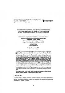
A GR control chart for detecting small shifts in mean is a combination of Shewhart’s barX chart and an extended version of CRL chart. It has a single horizontal line drawn at Y = L. Implementation of the GR chart is described as follows 1. Inspect n items produced in succession, which constitutes the respective group. ¯ sub chart. 2. Declare the group as conformed or non-conformed using X 3. A process is said to be out of statistical control, if either Y1 ≤ L or two successive Yr ’s are less than or equal to L for the first time. 4. When the process goes out of control, necessary corrective actions should be taken to reset and to resume it. Once the process restarts, move to Step 1. The above stepwise procedure can be explained with the help of flow chart given in Fig.1, where the counter K is used in such a way that K = 2 is an indication of out of control situation.

32

M.P. Gadre and R.N. Rattihalli

Figure 1: Flow-Chart of a Stepwise Procedure of Implementing GR Chart

The constants (n, k, L) that govern the implementation of the GR chart are known as design parameters of the chart and their optimal values can be obtained as discussed in the next section.

4

Design of GR Chart

In the synthetic control chart, for the same problem, Wu and Spedding [12] computed optimum values of control parameters (k, L) for given group size. In case of GR chart,

A Group Runs Control Chart for Detecting Shifts in the Process Mean

33

we find optimal choices of all the three parameters (n, k, L). In designing the GR chart, the model is Minimise ATS(δ 1 ) Subject to the constraint ATS(0)≥ τ

  (1)



Let P be the probability of the group being non conformed. Then     σ  ¯ ∼ N µ0 + δσ, √ ¯ < UX|S L)) P (N > r − 3)   = A2 (1 − A) 1 − P (N ≤ r − 3)  r−3

Ps = A2 (1 − A) 1 −

(6)

s=1

Thus, the probability distribution of N is given  A     0 Pr = P (N = r) = r−3   2  Ps  A (1 − A) 1 − s=1

Using the relations

∞  r=1

Pr = 1 and E(N ) =

∞  r=1

by, if r = 1 if r = 2

(7)

if r ≥ 3

rPr , it is easy to check that,

1 (8) A2 Hence, if a process signals out-of-control situation for the first time when N th nonconformed group is observed, then 1 n AT S(δ 1 ) = (9) P (δ 1 ) (1 − (1 − P (δ 1 ))L )2 E(N ) =

34

M.P. Gadre and R.N. Rattihalli

Thus, the optimisation problem (1) can be written in terms of (n, k, L) as Minimise P (δn 1 ) (1−(1−P1(δ ))L )2 1 Subject to the constraint 1 n ≥τ P (0) (1−(1−P (0))L )2

   (10)

 

A Method to Find Optimal Values of the Design Parameters (n, k, L) The optimisation search is carried out in three levels, namely, I. bottom level optimisation for L, II. second level optimisation for k, and III. top level optimisation for n. Bottom level optimisation for L From (10), it can easily be seen that, for fixed (n, k), both the functions ATS(0) and ATS(δ 1 ) are decreasing functions of L, L = 1, 2, . . .. Thus, the condition ATS(0) ≥ τ is satisfied for L = 1, 2, . . . , L∗(n,k) , where L∗(n,k) is such that 



nP (0)

L∗(n,k) 1 − 1 − P (0)

2 ≥ τ ≥ 

nP (0)  L∗(n,k) +1 2 1 − 1 − P (0)

Hence, from (10), the optimum value L∗(n,k) of L becomes    √ α ln 1 − CRL L∗(n,k) = 1 + ln(1 − P (0)) where, [a] denotes the largest integer not greater than a, and n αCRL = τ P (0)

(11)

(12)

(13)

Second Level Optimisation for k For fixed n, by considering the sub-domain   Dn = (n, k) : k > 0, AT S(0) ≥ τ , L = L∗(n,k)

(14)

one can search for the optimum point (n, kn∗ ) in the domain Dn at which ATS(δ 1 ) is minimum.

A Group Runs Control Chart for Detecting Shifts in the Process Mean

35

Top Level Optimisation for n For each n, starting from n = 1, considering the domain   D = n : 1 ≤ n ≤ m, AT S(0) ≥ τ , k = kn∗ , L = L∗(n,k)

(15)

the best choice of n which minimises ATS(δ 1 ) over the domain D can be obtained. Here, m is the smallest value of ATS(δ 1 ) ever attained. As ATS(n) ≥ n, while searching for the optimal value of n, if [ATS1 (n)] + 1 = m, then there is no need to consider the values of n ≥ m. This fact can be used while obtaining the optimum value of n. To compare ¯ the performance of GR chart with the synthetic and Shewhart’s X-control charts some numerical illustrations are discussed in the next section.

5

Numerical Examples

5.1

Example 1

For the first example, the following in some sense standardized values µ0 = 0, σ = 1, δ 1 = 0.2 and τ = 10000 are considered. ¯ chart, For these input parameters, values of the control parameters for the Shewhart’s X synthetic chart and the GR chart along with respective ATS(δ 1 ) are as follows. Here the suffices are used to the parameters n, k, L and ATS(δ 1 ) to point out the related chart. ¯ chart: nX¯ = 186, kX¯ = 2.35, ATSX¯ (δ 1 ) = 288; 1. Shewhart’s X 2. Synthetic chart: nS = 102, kS = 1.94 LS = 4, ATSS (δ 1 ) = 201; 3. GR chart: ng = 98, kg = 1.59, Lg = 3, ATSG (δ 1 ) = 165. This example shows that, not only ATSG (δ 1 ) is less than ATS of the other two charts, but also the group size ng of the GR chart is not exceeding the group sizes of the remaining two charts. ¯ chart and synthetic chart, for For further comparison of GR chart with Shewhart’s X various values of δ, the normalised ATS (normalised with respect to the synthetic chart) ¯ and GR charts by varying values from 0 to 3. For values are computed for both X synthetic chart the normalized ATS is always unity. The values are given in Table 1, entries up to δ = 0.68 are listed. For the larger values of δ, the values of normalised ATS for all the three charts are same as those for δ = 0.68.

36

M.P. Gadre and R.N. Rattihalli

¯ Table1: Performance of the GR Chart, Shewhart’s X-Chart and Synthetic Chart for Various Values of δ δ .00 .01 .02 .03 .04 .05 .06 .07 .08 .09 .10 .11 .12 .13 .14 .15 .16 .17 .18 .19 .20 .21 .22

ATSX ATSS ATSG δ ATSX ATSS ATSG δ .9998 1 1 .23 1.489 1 .8348 .46 .9862 1 1.001 .24 1.509 1 .8420 .47 .9552 1 1.004 .25 1.530 1 .8495 .48 .9264 1 1.004 .26 1.551 1 .8573 .49 .9122 1 1.000 .27 1.572 1 .8649 .50 .9158 1 .9898 .28 1.595 1 .8724 .51 .9349 1 .9735 .29 1.617 1 .8796 .52 .9659 1 .9531 .30 1.639 1 .8863 .53 1.005 1 .9306 .31 1.661 1 .8926 .54 1.049 1 .9080 .32 1.682 1 .8983 .55 1.095 1 .8865 .33 1.702 1 .9034 .56 1.141 1 .8673 .34 1.720 1 .9079 .57 1.186 1 .8509 .35 1.736 1 .9119 .58 1.228 1 .8375 .36 1.751 1 .9154 .59 1.267 1 .8271 .37 1.764 1 .9183 .60 1.303 1 .8197 .38 1.775 1 .9209 .61 1.334 1 .8149 .39 1.785 1 .9230 .62 1.363 1 .8126 .40 1.793 1 .9247 .63 1.388 1 .8125 .41 1.799 1 .9262 .64 1.410 1 .8143 .42 1.805 1 .9273 .65 1.431 1 .8177 .43 1.809 1 .9283 .66 1.451 1 .8224 .44 1.813 1 .9290 .67 1.470 1 .8282 .45 1.815 1 .9296 ≥ 0.68

ATSX ATSS ATSG 1.817 1 .93004 1.819 1 .93039 1.820 1 .93065 1.821 1 .93085 1.822 1 .93010 1.822 1 .93111 1.823 1 .93119 1.823 1 .93124 1.823 1 .93128 1.823 1 .93131 1.823 1 .93133 1.823 1 .93135 1.823 1 .93136 1.823 1 .93136 1.823 1 .93137 1.824 1 .93137 1.824 1 .93137 1.824 1 .93137 1.824 1 .93137 1.824 1 .93137 1.824 1 .93137 1.824 1 .93137 1.824 1 .93137

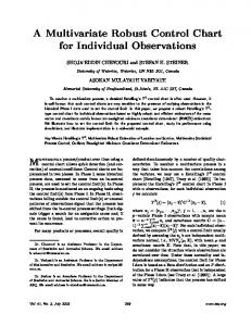
The graphs of normalised ATS against values related to the data in Table 1 are given in Fig. 2, from which it is observed that for δ > 0, except for very small values of δ we have ATSg (δ) < ATSs (δ) and ATSg (δ) < ATSX¯ (δ). Thus, the GR chart detects a shift ¯ chart, though of any size in the process mean earlier than the synthetic chart and the X optimum values of the design parameters are computed for a specific δ value. 5.2

Example 2

Here, an experiment similar to a 32 factorial experiment is carried out to compare the performance of the three control charts corresponding to 9 various combinations of input parameter values (δ 1 , τ ) and to study their effect on the performance of GR chart. The following combination of input values are selected: δ 1 : 0.2 τ : 2000

0. 5 10000

1 50000

A Group Runs Control Chart for Detecting Shifts in the Process Mean

37

Figure 2: The ATS-curves of the Three Chart-Types as function of δ

Considering all possible 9 combinations of the input parameters (δ 1 , τ ), values of the design parameters along with respective values of ATS(δ 1 ) are computed for each of the three control charts and are given in the following tables.

Table 2(A): Example Number and the Related Pair of Input Parameters and Average of Normalised ATS of the Three Charts Ex.

δ1

τ

1. 2. 3. 4. 5. 6. 7. 8. 9.

0.2 0.5 1.0 0.2 0.5 1.0 0.2 0.5 1.0

2000 2000 2000 10000 10000 10000 50000 50000 50000

Average of Normalised ATS Varying δ from 0 to 3 ¯ X-Chart Synthetic Chart GR Chart 1.182943 1.0 0.691257 1.578861 1.0 0.854673 1.565311 1.0 0.852664 1.762817 1.0 0.925964 1.676269 1.0 0.846491 1.557195 1.0 0.822583 1.753427 1.0 0.865199 1.759018 1.0 0.838845 1.599919 1.0 0.820088

38

M.P. Gadre and R.N. Rattihalli

Table 2(B): The Optimum Values of Design Parameters and ATS(δ 1 ) of the Three Charts Ex. 1. 2. 3. 4. 5. 6. 7. 8. 9.

n 112 32 11 186 45 14 269 59 18

¯ X-Chart k ATS(δ 1 ) 1.91103 192.6169 2.408924 48.29636 2.776214 15.59083 2.353445 287.984 2.840825 64.64391 3.194727 19.77997 2.783345 389.6462 3.243622 81.40963 3.56813 23.99978

n 95 19 6 102 25 8 149 31 10

Synthetic Chart k L ATS(δ 1 ) 1.49541 3 145.65108 1.896124 3 33.00241 2.142692 3 10.2286 1.938719 4 201.2094 2.179485 3 42.16538 2.398435 3 12.46769 2.144501 3 255.9365 2.445115 3 51.56039 2.643786 3 14.73389

n 63 16 5 98 21 6 129 26 8

GR Chart k L ATS(δ 1 ) 1.456995 4 123.5762 1.629960 3 27.2182 1.822851 3 8.202795 1.594030 3 164.4355 1.850151 3 33.6900 2.036518 3 9.8458 1.817895 3 204.9454 2.056836 3 40.1226 2.217812 3 11.41846

Since these 9 cases cover almost all the practical situations, we can conclude the following. 1. ng ≤ ns ≤ nX¯ 2. ATSg (δ 1 ) < ATSs (δ 1 ) < ATSX¯ (δ 1 ) 3. In each case, the average normalised ATS of GR is less than that of the other two charts. Thus, we conclude that GR performs uniformly better than synthetic and chart. The marginal graphs given in Fig. 3 are useful to study the effect of τ and δ 1 on GR chart. From Fig. 3, it is observed that for large values of τ and δ 1 , a GR chart is more effective. Figure 3: Normalized ATS as Function of τ and δ

It is to be noted that the run length based charts are not having single initial state. Therefore, it is necessary to study their performance in steady state and should be compared

A Group Runs Control Chart for Detecting Shifts in the Process Mean

39

with that of the compatible charts. In the following section we study such performance of the GR chart.

6

Runs Rules Representation and Steady State ATS Performance of GR Chart

Davis and Woodall [4] have discussed the runs rules representation of the synthetic control chart identifying shifts in the process mean depending on the X-based procedure. Here, we discuss the runs rule representation of a GR chart, using the group run lengths. Let the values of CRL be classified as ’0’ and ’1’ according as CRL > L and CRL ≤ L. Thus, the sequence of CRLs can be represented as a string of zeros and ones. For example, consider the sequence 0100011. This sequence indicates that among seven given values of CRL, only Y2 , Y6 and Y7 not exceeding L. If it is assumed that the value of CRL (say, Y0 ) at time zero satisfies Y0 ≤ L, then the GR chart is identical to the following runs rule. “Declare the process as out of control if two successive Yr s are less than or equal to L”. Thus, GR chart is identical to the above stated runs rule with the head start (Y0 ≤ L). The formula for ATS can be easily obtained by using the transition probability matrix (t.p.m.) of an absorbing Markov chain based on CRL values used to model the GR chart. If m = {Y > L} and  = {Y ≤ L}, then following t.p.m.is obtained related to the GR chart. m  Signal m 1−A A 0 (16)  1−A 0 A Signal 0 0 1 According to the runs rule representation of GR chart, it is clear that  corresponds to the initial state. Let R be the matrix obtained by deleting the last row and column of the above matrix. Then, the average number of defective groups observed before declaring the process as out of control is identical to the average time for the Markov chain to enter the absorbing state. The vector of average times corresponding to the various initial states is given by E(N ) = (I − R)−1 1

(17)

where 1 is a column vector of order two having all elements unity. The second element of E(N ) is A12 . Since a GR chart can be represented as a Markov chain, as noted by Davis and Woodall [4], it is desirable to study its performance in steady state. If the process is running smoothly for some time, the steady state ATS measures average time to signal, when the effect of head start has been demolished.

40

M.P. Gadre and R.N. Rattihalli

One may study the steady state performance of GR chart by using the above CRL based t.p.m., if the states are defined by considering the CRL values of the groups. To carry out ¯ chart in steady state the Markov chain representation of a comparison of GR with the X ¯ based procedure is needed. the GR chart depending on X Let the groups be classified as ’0’ or ’1’ according as conformed or non conformed and for illustration purpose assume that L = 3. Thus the GR chart will produce a signal if Y1 or two successive r s are less than or equal to 3. Let C and D be respectively the probabilities of the group being conformed and non conformed. As in Davis and Woodall [4] a Markov chain representation in this situation can be described by using the 14 states listed and the t.p.m. given below. Table 3: The States of the 1 000 2 0001 3 00010 4 000100 5 00011 6 000101 7 0001001

Markov Chain and their Labels 8 000110 9 0001010 10 00010010 11 0001100 12 00010100 13 000100100 14 Signal

In the above table, State 1 indicates that by now more than or equal to three (which is the value of L) conforming groups are observed, while State 2 indicates that a nonconforming group being observed after a sequence of at least three conforming groups. State 14 (signal) is a absorbing state. It indicates sequences of 0s and 1s ending with 1 and the current and the previous run length not exceeding L. The other states are non-absorbing states, which are accessible from State 2. The related one step t.p.m. is given below. 1 1 2 3 4 5 6 7 8 9 10 11 12 13 14

                       

2

3

4

5

6

7

8

9 10 11 12 13 14

 C D 0 0 0 0 0 0 0 0 0 0 0 0 0 0 C 0 D 0 0 0 0 0 0 0 0 0   0 0 0 C 0 D 0 0 0 0 0 0 0 0   C 0 0 0 0 0 D 0 0 0 0 0 0 0   0 0 0 0 0 0 0 C 0 0 0 0 0 D   0 0 0 0 0 0 0 0 C 0 0 0 0 D   0 0 0 0 0 0 0 0 0 C 0 0 0 D   0 0 0 0 0 0 0 0 0 0 C 0 0 D   0 0 0 0 0 0 0 0 0 0 0 C 0 D   0 0 0 0 0 0 0 0 0 0 0 0 C D   C 0 0 0 0 0 0 0 0 0 0 0 0 D   C 0 0 0 0 0 0 0 0 0 0 0 0 D   C 0 0 0 0 0 0 0 0 0 0 0 0 D  0 0 0 0 0 0 0 0 0 0 0 0 0 1

(18)

A Group Runs Control Chart for Detecting Shifts in the Process Mean

41

For the general value of L, the matrix R1 (eliminating the last row and the last column of the t.p.m.) has the following states. 1. A sequence of L zeros; State 1 in the above example. 2. Sequences of L zeros followed by 1 and further appended by at most (L - 1) zeros. There are L such sequences; States 2,3 and 4 in the above example. Thus, such type of states are 3 ( = L)). 3. Each of the sequences in (2) followed by 1 and is further appended by a sequence of at most (L - 1) zeros. The total number of such sequences is L2 ; States 5 to 13 in the above example. Thus, such type of states are 9 ( = L2 )). Therefore, R1 is a square matrix of order 1 + L + L2 = L(L + 1) + 1

(19)

Note that the (i, j)th element of R1 is  C if the ith state leads to the jth state,     which corresponds to a sequence ending with ’0’  D if the ith state leads to the jth state, R1 (i, j) =   which corresponds to a sequence ending with ’1’    0 otherwise

(20)

Let π be a 1 × (L(L + 1) + 1) row vector corresponding to the stationary probability distribution that the Markov chain will be in each of the non absorbing states, which is conditioned on no signal. Then the steady state ATS of the GR chart can be obtained after multiplying by ng to the product of π and ARL, where ARL can be obtained by (I − R1 )−1 1. It is to be noted that for any run length based control chart, the steady state ATS is not smaller than zero state ATS. If the signal depends on one point only, both ATS’ are same. Hence the performance of the two charts should be compared by making the (S.S. ATS)0 of the two charts same. Hence we compute adjusted steady state ATS of the chart II with respect to the chart I as [Adj. S.S. ATS(δ)]II =

[S.S. ATS(δ)]II [S.S. ATS(0)]I [S.S. ATS(0)]II

(21)

Example 1 (Cont.): The following table gives the steady state ATS and the adjusted steady state ATS values corresponding to various values of δ of Example 1 for all the three charts.

42

M.P. Gadre and R.N. Rattihalli

Table 4: Values of Steady State (ATS) Corresponding to Various δ Values for the Three Charts Considered in Example 1 δ [S.S.ATS]X¯ 0 9999.825 0.1 1153.281 0.2 287.984 0.26 210.5349 0.3 193.9732 0.4 186.1791 0.5 186.0007 0.6 186 0.7 186

[S.S.ATS]S 11725.36 1426.76 284.51 177.3712 148.52 123.3 122.55 122.4 122.4

Adj[S.S.ATS]S 10000 1247.518 242.645 151.2714 126.6656 106.8624 104.517 104.389 104.389

[S.S.ATS]G 13531.00 1580.59 306.36 204.6359 178.62 158.91 156.89 156.8 156.8

Adj[S.S.ATS]G 10000 1168.125 226.4134 151.2349 132.008 117.4414 115.9486 115.882 115.882

From the above table, we conclude that for small to moderate shifts (in this example up to δ = 0.26 = (δ  > δ 1 , say)) in the process level, the steady state performance of GR is better than that of the two other charts. Remark: Due to advancement in engineering technology, very rarely the process level shoots up beyond the level δ  (measured in terms of σ). As such a producer would like ¯ In these situations a GR to detect even small to moderate shifts in the process mean X. chart is superior to the other two.

7

Conclusions

¯ chart or a A GR control chart proposed here performs significantly better than an X synthetic chart. The ATS(δ 1 ) is significantly less than that for the other two charts. Also in the steady state GR performs better in detecting small to moderate shifts than the remaining two charts. Though the discussion in this paper is based on 100% inspection, the chart can also be applied to non-100% inspection cases if uniform sampling is adopted. By uniform sampling we mean inspecting the units at equal time intervals (in terms of the number of units). Acknowledgement: The first author is grateful to the UGC New Delhi for awarding the ’Teacher fellowship’ to complete his research work. We are thankful to both the referees for their valuable comments and suggestions, which helped a lot to improve the manuscript. We are also thankful to the regional and the managing editor for their quick response. We are thankful to Prof. Wu for providing a computer program a− synth.c of computing control parameters of the synthetic chart. We are also thankful to Prof. Davis and Prof. Woodall for sending their manuscript.

A Group Runs Control Chart for Detecting Shifts in the Process Mean

43

References [1] Albin, S. L.; Kang, L. and Shea, G. (1997): An X and EWMA Chart for Individual Observations. Journal of Quality Technology 29, 41-48. [2] Bourke, P. D. (1991). Detecting a Shift in Fraction Nonconforming Using RunLength Control Charts with 100% Inspection. Journal of Quality Technology 23, 225-238. [3] Champ, C. W. and Woodall, W. H. (1987). Exact Results for Shewhart’s Control Charts with Supplementary Runs Rules. Journal of Quality Technology 19, 388-399. [4] Davis, R. B. and Woodall, W.H. (2002). Evaluating and Improving the Synthetic Control Chart. Journal of Quality Technology 34, 63-69. [5] Gadre, M. P. and Rattihalli R. N. (2004): A Group Runs Control Chart to Identify Increases in Fraction Non-Conforming (Submitted to JSCS) [6] Kaminsky, F. C., Benneyan, J. C. and Davis, R. B. (1992). Statistical Control Charts Based on a Geometric Distribution. Journal of Quality Technology 24, 63-69. [7] Lucas, J.M. and Saccucci, M.S. (1990): Exponentially Weighted Moving Average Control Schemes: Properties and Enhancements. Technometrics 32, 1-12. [8] Montgomery, D. C. (1996). Introduction to Statistical Quality Control. John Wiley & Sons, New York. [9] Ncube, M. M. (1990): An Exponentially Weighted Moving Average Combined Shewhart Cumulative Score Control Procedure. International Journal of Quality and Reliability Management 7, 29-35. [10] Roberts, S.W. (1959): Control Chart Tests Based on Geometric Moving Averages. Technometrics 1, 239-250. [11] Shamma, W. E. and Shamma, A. K. (1992): Development and Evaluation of Control Charts Using Double Exponentially Weighted Moving Averages. Journal of Quality and Reliability Management 9, 18-25. [12] Wu, Z. and Spedding, T. A. (2000). A Synthetic Control Chart for Detecting Small Shifts in the Process Mean. Journal of Quality Technology 32, 32-38. [13] Wu, Z. and Spedding, T. A. (2000). Implementing Synthetic Control Charts. Journal of Quality Technology 32, 75-78.

M.P. Gadre Department of Statistics Mudhoji College, Phaltan, Pin - 415523, INDIA mpg28@rediffmail.com

R.N. Rattihalli Department of Statistics Shivaji University, Kolhapur Pin-416004, INDIA rnr5@rediffmail.com