A Growth Algorithm for Neural Network Decision Trees Mostefa Golea and Mario Marchand∗ Department of Physics, University of Ottawa, 34 G. Glinski, Ottawa, Canada K1N-6N5 PACS. 02.70 - Computational techniques. PACS. 87.10 - General, theoretical, and mathematical biophysics (inc. logic of biosystems, cybernetics and bionics).
Accepted by Europhysics Lett.; March 12, 1990
Abstract This paper explores the application of neural network principles to the construction of decision trees from examples. We consider the problem of constructing a tree of perceptrons able to execute a given but arbitrary Boolean function defined on Ni input bits. We apply a sequential (from one tree level to the next) and parallel (for neurons in the same level) learning procedure to add hidden units until the task in hand is performed. At each step, we use a perceptron-type algorithm over a suitable defined input space to minimise a classification error. The internal representations obtained in this way are linearly separable. Preliminary results of this algorithm are presented.
1
Introduction
Feed-forward layered neural networks[1, 2] are in principle able to learn any arbitrary mapping provided that enough hidden units are present[3]. A way to improve the performance of a neural network is to match its topology to a specific task as closely as possible. However, the determination of the optimal number of hidden units and the optimal net topology is still an open question. More than that, it has been shown recently [4, 5] that the problem of deciding whether or not a given mapping can be performed by a given architecture is NP-complete. Contrary to the standard procedures like back-propagation[1], ∗ E-mail:
[email protected]
M. Golea and M. Marchand
2
the approach adopted in this paper is very similar in spirit to some recently developed heuristics of inferring networks from the sample data[6, 7, 8, 9]: rather than fixing the architecture in advance, the hidden units are added one by one following some rules until the given task is performed. Since many problems are easily represented by multi-branched decision procedures, the design of efficient decision trees from data is currently an important topic in several fields[10]. Given that the optimal tree derivation is NPcomplete[11], we are led to consider the possibility of heuristic algorithms for constructing neural decision trees from examples. The basic idea behind the present approach is that it is possible to choose the connection between each tree node in such a way that each node needs to try to classify only one of the two decision regions of his parent. Since at each layer, the number of patterns needed to be classified decreases (typically by half), the growth process is guaranteed to stop. Moreover, we show that the set of internal representations occurring on the leaves of the tree is always linearly separable and thus, we can always easily find a set weights going from the leaves to the output unit in order to perform the desired Boolean function.
2
The growth algorithm for the perceptron tree
Consider a Boolean function defined on M (distinct) patterns {ξ~µ }µ=1,...,M of Ni binary input units ξjµ = ±1, (j = 1, . . . , Ni ) whose value is given by the targets σ µ = ±1. The function is not necessarily defined on all the 2Ni possible patterns so we have M ≤ 2Ni . We want to find a neural tree of L layers (L = 1, 2, . . .), each layer being made of at most 2L−1 hidden units (see Fig. 1). We will construct level L from level (L − 1) in the following way : depending on the form of its decision regions (see below), each hidden unit in level (L − 1) will generate (and be connected with) either 2 units in level L (if it is a non-terminal node), 1 unit (semi-terminal node) or no node at all(terminal node). The first hidden unit (the root) receives its inputs only from the input units while all the other hidden units are, in addition, connected to all their ancestors. The terminal nodes and some of the semi-terminal nodes will be connected to the output unit. If we denote by wk,j the connection going from input unit j to hidden unit k,and by vk,i the connection from hidden unit i to hidden unit k, the output Skµ of hidden unit k, when pattern ξ~µ is presented to the net, is given by: Ni X X wk,j ξjµ + vk,i Siµ ), Skµ = sgn( j=0
(1)
i∈A(k)
where the summation over i runs over all the ancestors of hidden unit k and wk,0 is the bias of unit k.
M. Golea and M. Marchand
3
The algorithm essentially deals with one tree node at a time. For each node k, we first find the the weight vector w ~ k (coming from the input units) that minimises an error defined on a (wisely chosen) subset of input patterns. For that purpose we have chosen a variant of the perceptron algorithm called the pocket algorithm[12] which allows us to find a ”good” solution even in the nonlinearly separable case if we let it run for a sufficiently long time1 . If this subset N(k) of input patterns contains Nk+ positive target patterns and Nk− negative target patterns, we have chosen to minimise the following error (for node k): Ek = (
m+ m− k k + ), N +k Nk−
(2)
− where m+ k (mk ) stands for the number of misclassified positive (negative) target patterns by node k. Having obtained w ~ k by this error-minimisation procedure, we define the k + (k − ) decision region of neuron k by the subset of patterns in N(k) for which we have Skµ = +1 (−1). Next, we will determined the type (terminal, non-terminal or semi-terminal) of node k according to these four possible outcomes: − + and k − ) defined 1. m+ k 6= 0 and mk 6= 0. The two decision regions (k by neuron k are ”mixed” (ie. each of them contains patterns of different targets). We then declare node k to be a non-terminal node and in the next level it will generate and be connected to two ”offspring” neurons. The ”right offspring” will try to ”purify” the k + region and his training set will consist only of these patterns. The ”left offspring” will try to ”purify” the k − region and his training set will consist only of these patterns. − 2. m+ k = 0 and mk = 0. The two decision regions defined by k are ”pure” (ie. each of them contains patterns of one target only). The neuron k is a terminal-node. It is connected to the output. No neuron is generated for this node in the next level. − 3. m+ k = 0 and mk 6= 0 . The neuron is a semi-terminal node because only the k + region needs to be ”purified”. Hence, neuron k will be connected to a right offspring whose training set will be the k + region only. Since the k − region is ”pure”, neuron k will be connected to the output unit. + 4. m− k = 0 and mk 6= 0. The neuron is a semi-terminal node because only − the k region needs to be ”purified”. Hence, neuron k will be connected to a left offspring whose training set will be the k − region only. Neuron k will not be connected to the output unit because the k − region is ”mixed”.
Hence, the training set of a ”right offspring” (”left offspring”) neuron will consist only of the k + (k − ) decision region of his parent. It will become clear below why we choose to connect to the output unit only the nodes whose k− decision region is ”pure”. 1 But
we do not know how long we need to wait in general.
M. Golea and M. Marchand
4
Next, we need to describe how we choose, for each node k, the connections to his ancestors. First note that if unit k is located at layer L, it has L − 1 ancestors that we label by 1, 2, · · · L − 1 (starting with the youngest). Having found, by the error-minimisation procedure, the weight vector w ~ k , we choose the vk,i ’s and renormalize the bias according to these rules: 1. |vk,i | = 1 +
PNi
j=0
|wk,j |,
for i = 1 . . . L − 1.
2. vk,i is positive (excitatory) if unit k is located in the left sub-tree having unit i as a root. Else, it is negative (inhibitory). PL−1 3. We renormalize the bias of k according to: wk,0 → wk,0 + i=1 |vk,i |. This choice ensures that node k will always have Skµ = +1 whenever pattern µ does not belong to his training set. Indeed, one can easily verify (using Eq. 1) that all patterns µ belonging to the i− decision region of ancestor i of k will have Skµ = +1 if k is in the right sub-tree having unit i as a root, and that all patterns µ belonging to the i+ decision region will have Skµ = +1 if k is in the left sub-tree having unit i as a root. It is important to mention that this property can be achieved by other choices than these ones above. Our growth algorithm is then the following: 1. To find the root node (and his weight vector w ~ 1 ), run the pocket algorithm to minimise the classification error over the initial set of data. Determine the type of the node (terminal, semi-terminal or non-terminal). Stop if it is a terminal node. Otherwise go to step 2. 2. Create a new layer by generating the required number of units according to the type of the units in the layer below. Then, for each unit of this new layer: a) Determine its training set according to the rule above. b) Run the perceptron-pocket algorithm (on the wk,i only) to minimise the error on its training set. c) Determine the value of each vk,i coming from all its ancestors and renormalize wk,0 according to the three rules above. d) Determined the type of each node according to the four cases above. 3. If all units of this layer are terminal nodes, stop. Otherwise, go back to step 2. The process is sequential in the sense that all units in Level L have to be dealt with before we can build level (L + 1), and is parallel in the sense that we can deal with all units of one level at the same time. This growth process will eventually stop because the training set of each unit will be lower (by at least one pattern) than the training set of his parent. Suppose that after this growth process we have N tree nodes (the leaves) connected to the output. Upon presentation of input pattern ξ~µ to the net, the
M. Golea and M. Marchand
5
~ µ that we call the internal represenoutput of these leaves will form a vector S µ tation of pattern ξ~ . If we denote by uj the connection going from leaf j to the output unit and u0 its bias then, upon presentation of pattern ξ~µ to the net, the state of the output unit is given by: N X uj Sjµ + u0 ). Oµ = sgn(
(3)
j=1
The original Boolean function has now been mapped into a new function defined by the internal representations. We now prove that: the set of internal representations obtained by this growth algorithm is linearly separable. Better, we will write down the solution for the weight vector ~u. First note that by this process of giving, at each node, one decision region to the left offspring and the other to the right offspring until a pure region is found; each input pattern ξ~µ has been associated to a unique terminal or semi-terminal node. Since all leaves have pure k − regions, they will all, except one, be forced to a +1 output when a negative target pattern is presented to the net. If, however, a positive target pattern is presented to the net, all leaves, without exceptions, will have a +1 output. Note that this would not have been the case if semi-terminal nodes having ”mixed” k − regions would have been leaves (and connected to the output unit). This is why it is necessary not to connect these semi-terminal nodes to the output. Hence, upon the presentation of any pattern ξ~µ , the internal representation vector has the form: ~ µ = (1, 1, . . . , 1, σ µ , 1, . . . , 1). S
(4)
Hence, the desired output of this vector is always obtained if we choose: uj u0
= =
1 f or j = 1, . . . , N −(N − 1)
(5) (6)
which can be directly verified (by using eq. 3, 4, 5 and 6).
3
Simulations results
Random Boolean Functions. To test the robustness of the algorithm, we have generated, at random, 100 Boolean functions on 6 input bits. As expected, a neural tree was always found that performed the task. The average number of hidden units found was 20.5 ± 3.9 which is very similar to the one obtained by another growth algorithm[6] whose strategy is also to minimise an error. But the network architecture is quite different. Parity function. For this task the output of Ni input bits must be +1 if the number of +1 input bits is odd, and −1 otherwise. For Ni = 2, . . . , 8,
M. Golea and M. Marchand
6
the number of hidden units generated was always equal to Ni . An example is ~ k are shown in Fig. 2 for Ni = 4. Notice that all the input connection-vectors w parallel. This illustrates the fact that the boundaries between positive target and negative target patterns are parallel planes[3, 7].
4
Conclusion
In summary, the sequential-parallel algorithm outlined in this paper identify a new class of procedures that will build a neural tree able to map any Boolean function defined on a given sample data. This algorithm possess a lot of freedom in the way the inter-node connections may be chosen; we have presented here only one possibility. In addition, learning occures only at the single neuron level and our algorithm can accomodate any variants in the way to choose the incomming weight vector w. ~ Here we have decided to find the w ~ that minimises an error but it would be interesting to consider other criteria like maximum of mixing entropy[13] or the maximum cluster size[8]. This work is still in his infancy and more test are needed on many other problems. Results on the ”generalization” ability of this algorithm will be presented in a near future. note added: After submission of this paper for publication, we received a preprint of a related work by J. A. Sirat and J. P. Nadal. The key idea that the training set of each neuron consist only of patterns belonguing to one decision region of his parent is present in both approaches. However, as they themselves indicate, they obtain a tree of neurons, not a neural network (like in our procedure) since they do not have any weight values connecting their tree nodes. Interestingly, they have generalize their algorithm to handle multiclass problems. Their idea of performing a principal axis dichotomy on the classes could be implemented in our procedure.
References [1] D. E. Rumelhart, J. L. McClelland, Parallel Distributed Processing Vol. 1-2, (Bradford Books, MIT Press, Cambridge , Ma., 1986). [2] J. Denker, D. Schwartz, B. Wittner, S. Solla, J. Hopfield, R. Howard, L. Jackel, Complex Systems 1, 877-922 (1987). [3] M. L. Minsky, S. Papert, Perceptrons: an Introduction to Computational Geometry, (exp. ed.), (MIT Press, Cambridge, MA., 1988). [4] S. Judd, Proc. IEEE First Conference on Neural Networks, San Diego 1987, (IEEE Cat. No. 87TH0191-7, Vol. II 685-692). [5] A. Blum and R. L. Rivest Proceedings of the first workshop on computational learning theory, Morgan Kaufmann, 9-18 (1988).
M. Golea and M. Marchand
7
[6] M. M´ezard, J.P. Nadal, J. Phys. A, 22, 2191-2203 (1989). [7] P. Ruj´ an, M. Marchand, Complex Systems 3, 229–242 (1989). Proceedings of IJCNN 1989, Washington D.C, Vol II. 105-110. [8] M. Marchand, M. Golea and P. Ruj´ an, Europhys. Lett, (in press). [9] J.P. Nadal, International Journal of Neural Systems 1, 55 (1989). [10] L. Breiman, J. H. Friedman, R. A. Olshen and C. J. Stone, Classification and Regression Trees. (Wadsworth, Belmont CA, 1984). [11] L. Hyafil and R. L. Rivest, Inform. Process. Lett. 5, 15-17 (1976). [12] S. I. Gallant, IEEE Proc. 8th Conf. on Pattern Recognition, Paris (1986). [13] R. Linsker, Computer21, 105–117 (1988).
M. Golea and M. Marchand
8
11
10
5
6
7
3
8
9
4
2 1
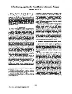
Figure 1: Scheme of the proposed neural network tree. It consists of Ni input, one output and yet an unspecified number of hidden units organised in a hierarchical way. Each hidden unit is connected to the inputs (in the lowest layer) and to all its ancestors. Unit 1 is the root node. Unit 6 and 8 are terminal nodes, unit 5 and 7 are semi-terminal nodes and unit 2, 3 and 4 are non-terminal nodes (see text below). Our growth algorithm is such that each inter-node connection coming from an ancestor located to the right is excitatory whereas if it comes from an ancestor located to the left, it is inhibitory. The connections going to the output unit (not shown) are ”arrowed”. For clarity, only part of the tree is shown.
M. Golea and M. Marchand
9
-2
1
1
1 19 -8 8 -1
-1
1
9 11 2
-1
2
-2
-1
1 11
-8
-1 -2
1
1
1
-1
-1
1
Figure 2: A network obtained by our algorithm on the parity task. The bias values of the neurons are indicated in the circles. For clarity, the connections coming from the input units have been interrupted (except for the root).