A Hard Real-Time Static Task Allocation Methodology for Highly-Constrained Message-Passing Environments B. Earl Wells Department of Electrical and Computer Engineering The University of Alabama in Huntsville Huntsville, AL 35899 Phone (256) 824-6047 FAX (256) 824-6803
[email protected] Index Terms: Parallel Processing, Real-Time Systems, Scheduling Theory, Simulation
Abstract This paper presents a method of exploiting the functional parallelism present within a class of well-defined deterministic software systems to achieve real-time execution on a highlyconstrained MIMD message-passing architectural model. The methodology is targeted to software systems that do not respond well to conventional data parallel techniques because of the irregular flow of data resulting from their structure. Such software systems are assumed to be composed of computational and i/o processes (tasks) that execute in a periodic manner under hard real-time constraints. The method performs automatic assignment, mapping, and scheduling of these tasks to the available set of processors assuming a reduced complexity hardware configuration that employs synchronous non-buffered (lock-step) communication between the sending and receiving processors, and simple store-and-forward routing of messages between processors. This methodology is unique in that it combines simulated annealing with a newly developed listbased heuristic to obtain very good solutions in the majority of cases. The effectiveness of the method has been illustrated by applying it to a large number of randomly generated task systems and to a real-world simulation of a U.S. Space Shuttle Main Rocket Engine.
1 B. E. Wells -- The International Journal of Computers and Their Applications, Vol. II, No. 3, December 1995.
1: Introduction Consider a well-defined system of heterogenous processing tasks that exhibit deterministic behavior and are activated periodically during program execution. Also assume that this set of tasks interact with each other in an irregular manner, making parallelization very difficult using conventional data parallel techniques. An example of such a configuration is illustrated pictorially in Figure 1, where the nodes represent computational tasks (i.e. portions of a program that must I2
T4 5
I1
T3 4
T9 2
T1 2
T7 6
T14 2
T2 5
T6 1
T5 2
T8 5
T12 3
I3
T10 9
T15 4
T11 3
T13 3
O2 O1 Figure 1: Task Graph for Well-Defined Deterministic System execute serially with no part executing in parallel) and the weights being assigned reflect the computational complexity of each of the tasks. For this well-defined software system, it is assumed that once task execution has begun it must continue uninterrupted until it is completed (i.e. the tasks are non-preemptive). The directed arcs between adjacent nodes describe the precedence relationships between the tasks with their weights representing the amount of data and/or control information that must be communicated between the tasks. It is assumed that such communication weights can vary but are generally small when compared to the amount of computation associated with the tasks. The model requires that only one data/control output is produced per task 2 B. E. Wells -- The International Journal of Computers and Their Applications, Vol. II, No. 3, December 1995.
and this output takes the form of a data token that is consumed in a data flow sense by all adjacent tasks in the task graph. While the aforementioned restrictions limit the applicability of this well-defined software model to only a subset of the problems which can potentially benefit from parallel processing, many important problems are members of this subset. Included in this subset are many hard realtime applications which incorporate data acquisition/control functions within a hardware-in-theloop type arrangement. It is these types of problems being addessed by methodologies presented in this paper. Consider also a highly-constrained hardware model of a message-passing architecture that has the following characteristics 1. the processors and communication network are homogeneous in speed and function, 2. communication between processors is totally synchronous utilizing blocking sends and blocking receives within a non-buffered statically-linked topology, 3. store-and-forward routing is employed to communicate messages to nonadjacent processors, 4. as a result of hardware simplification, computation and communication cannot be overlapped in time and, 5. the data acquisition/control devices that drive and respond to program execution are each connected to only one processor through local memory interfaces or remote data links that are separate from the interprocessor communication network. Unlike the general models used by parallel algorithm developers this hardware model is much more restrictive (and perhaps more realistic). The advantage of utilizing such a restrictive model is that software methodologies fashioned for this more restrictive environment will in many cases be applicable to less restrictive environments, but the reverse is rarely the case. The hardware model appears to be a good match to the aforementioned well-defined software system. Although the model is still an abstraction, it is very consistent with hardware architectures built from commercially available devices such as the INMOS series of Transputers. A potential advantage of such a simple hardware model is that performance gains over more complex hardware are possible in many instances by minimizing overhead incurred by
3 B. E. Wells -- The International Journal of Computers and Their Applications, Vol. II, No. 3, December 1995.
including inefficient and rarely used hardware. In manny cases special context switching, communication buffering, and message routing hardware can often be eliminated replacing it with hardware resources that might be more effective in increasing overall performance. As a case in point, consider the various forms of cut-through routing schemes that have been used in many proprietary multicomputing architectures. These schemes require that messages be divided into segments which are then pipelined through the network. Such routing mechanisms are very useful for many types of problems where large amounts of data are sent relatively infrequently. This is not a good match to the well-defined software systems which are discussed in this paper because small amounts of data are to be sent between tasks very frequently. In such cases, a simple store-and-forward routing format is often more efficient since message sizes are too small to benefit from pipelining and the store-and-forward routing hardware can be created in a manner that does not incur the various hardware/software penalties (such as added buffer delays) imposed in many cut-through routing implementations. Cut-through routing schemes can be very resource intensive requiring additional communication functional units/processors, a complex interrupt mechanism, and/or complex low-level software. Finally, many well-defined software systems display a locality-of-communication property that if recognized by the preprocessing allocation software would minimize the need for such complex hardware. An additional advantage of reducing hardware complexity is that application specific massively-parallel configurations can be created quickly utilizing existing uniprocessor technology or such configurations can be created utilizing moderate-complexity components that can be prototyped rapidly and inexpensively using field programmable logic devices. Furthermore, if processors are relatively simple, larger numbers of them can be encased in the same multichip modules resulting in greatly improved communication speed between the processors. The trade off is that much of the efficiency burden and complexity has been shifted from the hardware implementation onto the preprocessing software. An additional advantage of reducing hardware complexity is that a simplified model can be of great advantage when verifying the correctness of software operation in terms of meeting all timing requirements. Many aspects of more complex processors hinder the verification and vali4 B. E. Wells -- The International Journal of Computers and Their Applications, Vol. II, No. 3, December 1995.
dation of real-time systems. For example, the lock-step synchronization requirement of the highly-constrained hardware models eliminates the unpredictable operation of large message buffers, complex communication polling schemes, and/or special interrupt driven communication handlers. This paper is organized in ten sections. In Section 1 an overview and introduction of the well-defined software system and highly-constrained hardware model has been presented. The basic parameters being used throughout this paper and the necessary conditions to insure that real time constraints are met are described in Section 2. Section 3 discusses previous research in the area of task allocation (i.e. scheduling, assignment, and mapping). In Section 4, the SNBC allocation methodology is introduced to effectively merge the aforementioned software systems and hardware environments. The methodology employes a special-purpose communication insertion strategy (as is described in Section 5) to overcome much of the synchronization overhead caused by the non-preemptive task system. Section 6 is a detailed example of the mechanics of applying the SNBC methodology to a small software/hardware system. Simulated annealing is used to augment the base methodology in Section 7. The augmented methodology is then evaluated in Section 8 by applying it to a number of randomly-generated software systems assuming first a completely-connected topology and then an N-Cube topology. Similar analysis is performed in Section 9 when the combined methodology is applied to a simulation of a space shuttle main rocket engine. General conclusions are then presented in Section 10.
2: Basic Parameters The following terminology and definitions are used throughout this paper: Ftm
= Time Frame Requirement -- the maximum time allowed to execute one complete cycle of the periodic task graph (i.e. this is the longest permitted time to execute all the tasks in the underlying Directed Acyclic Task Graph, DAG, associated with the well-defined system),
m
= Number of Tasks in the system,
W
= Total Workload -- the total amount of computation to be performed to execute all the tasks in the underlying DAG (in appropriate units of instructions, floating-point operations, logical inferences, etc.), m–1
Wi
= Workload associated with each Task, Ti, where W =
∑ W i, i
5 B. E. Wells -- The International Journal of Computers and Their Applications, Vol. II, No. 3, December 1995.
ϒi
=
β
= Number of Task Types in the task graph where 0 ≤ β < m ,
Si
= Setup Time for Task i -- the time measured from the beginning of a time frame before which a task is not allowed to begin execution,
Ci,,j
= Communication Weight -- the amount of data that must be forwarded from task Ti to task Tj
n
= Number of Processors in the system,
Pj
= Processor j -- where 0 ≤ j < n ,
Ψ
= Nodal Execution Rate -- the computing capacity of each processing node (in appropriate units of MIPS, MFLOPS, MLIPS, etc.),
ζ
= Link Communication Rate -- the speed at which data can be transferred across nearest-neighbor links between processing element Pi to processing element Pj. It should be noted that even though the communication characteristics of each nearest-neighbor link are assumed to be identical ζ , is not a constant but is dependent upon the amount of data that is transferred,
Task Type -- the type of nonpremptive processing task i (distinguishes between the different types computational tasks and input/output operations),
Γ (pi,k) = Task Limit -- the number of tasks of a type, k, that can be executed on processor pi (This parameter is used to limit the number of special purpose tasks such as i/o tasks to processors that support their function), α
= Amdahl’s Fraction -- portion of the workload that must be executed sequentially,
ξ
= Task Graph Structure Parameter -- the parameter that describes the structure of a task graph with ξ = 0 representing a totally parallel graph and ξ = 1 a sequential graph. Note that this parameter is not the same as Amdahl’s fraction since all graphs of a given concurrency do not have identical properties (i.e. there are dense and sparse graphs with the same m and α ). An example of a methodology for approximating such a parameter is reflected in the calculation of alignment functions [1],
γ
= Allocation Parameter -- an abstract parameter that describes the degree of optimality associated with a given allocation of m tasks to a topology with n processing nodes,
κ
= I/O Structure Parameter -- an abstract parameter that describes the degree by which processors can concurrently access i/o devices to acquire or to output non-homogeneous data. It is a measure of the i/o structure and capabilities of the hardware architecture. Two extreme structures are represented by the share-all and share-nothing configurations. In a share-all type arrangement all i/o devices are connected via a common data link such as a global bus which is accessible by all processors in the system. In a share-nothing system each i/o device is connected directly to a processor through separate local buses. Most 6
B. E. Wells -- The International Journal of Computers and Their Applications, Vol. II, No. 3, December 1995.
systems display the characteristics that fall in between these two extremes, with a number i/o devices being connected to each processing element in a manner which allows multiple i/o operations to be performed in a time multiplexed manner. With these parameters defined it is clear that to ensure real-time execution, the following inequality must be guaranteed to hold true for each iteration αW --------- + Ω ( γ , ξ ) + com ( γ , ξ ) + io ( γ , ξ, κ ) ≤ F tm Ψ
(1)
The first term in the equation reflects the time spent doing useful computation during each iteration of software execution. This is the easiest of the four terms in the left hand side of the equation to compute for a given application. It represents the ideal time that one iteration of a given task graph can execute on a given architecture not taking into account the overheads associated with load imbalance, communication/synchronization latency, and i/o speed. If real time perαW formance is to be achieved, then for most applications --------- « F tm . Ψ The second term, Ω ( γ , ξ ) , is the load imbalance function which quantifies the effect of having uneven distribution of work among the processors. This term is dependent upon the task graph structure, widely varying task weights, a poor allocation of tasks to processors, or fewer than the minimum number of processors necessary to make use of the parallelism present in the task graph. In the case where ξ = 1 , and n = 1 (the sequential case) Ω ( γ , ξ ) = 0 . When ξ = 0 (the totally parallel case) the lower bound on the load imbalance function is 1 when n ≥ --Ω ( γ , ξ ) min = 0 α Ω ( γ , ξ ) min
(2)
W ( 1 – αn ) = --------------------------nΨ
when 1 ≤ n < --1α
When tasks are of relative equal complexity and n is less than m then Ω ( n, γ , ξ ) will be close to its lower bound for allocations produced by most allocation methodologies. The com ( γ , ξ ) function represents the time lost due to communication latency, channel bandwidth, and process synchronization. It is a measure of communication overhead. For the totally sequential case (where ξ = 1 and n = 1 ) and the parallel cases ( ξ = 0 ) then com ( γ , ξ ) = 0 . In all other cases, no closed-form solution for the lower bound of com ( γ , ξ ) can be expressed because it is dependent upon the topology and the allocation. 7 B. E. Wells -- The International Journal of Computers and Their Applications, Vol. II, No. 3, December 1995.
The last term in Equation 1, io ( γ , ξ, κ ) , represents the time lost due to the input and output of data from and to the real world. This represents an overhead function associated with the data acquisition and control functions of the hard real time system. If it is assumed that all i/o devices have been initialized to trigger simultaneously at the beginning of each time frame, then the i/o operations can be represented in the same manner on the highly-constrained model as the computational tasks, with i/o representing the relative CPU burden of an individual processor accessing the i/o device and the arc weights reflecting the amount of data that is transferred in the i/o operation. This implies that i/o devices connected to a processor must be accessed in a serial manner by that processor but that parallel accesses of i/o devices can occur when the set of i/o devices are spread out among the processors. It is also assumed that the i/o devices are capable of operating concurrently and independently after software initialization.
3: Related Research If it is assumed that there are relatively few feedback arcs associated with the communication between different iterations of the periodically executing task graph present in the welldefined software system, then a feasible paradigm is to temporarily remove these feedback arcs, allocate the directed acyclic portion of the task graph, reconnect the feedback arcs, and schedule all cross-iteration communications. An advantage of this paradigm is that there has been much research into the development of general methodologies which statically allocate (assign, map and schedule) directed acyclic task graphs to a network of processors. The following represents some algorithms which fall nicely into this classification. The general acyclic allocation problem is NP hard but there are a few optimal polynomialtime algorithms for special-case hardware systems. Algorithms of this type include those developed by Hu [2], Coffman and Graham [3], and Anger, Hwang, and Chow [4]. It is important to note that the restrictions imposed on the task system and targeted topology relegates the applicability of these methodologies to a small number of relatively unimportant special-case problems. The more general problem assumes an arbitrary number of processors, nonuniform task execution times, and a nonregular precedence structure, and can be solved in polynomial time by employing inexact algorithms based upon various heuristics. Many of these algorithms are based upon the 8 B. E. Wells -- The International Journal of Computers and Their Applications, Vol. II, No. 3, December 1995.
assumption that communication delay is negligibly small, such as may be the case for certain coarse-grained systems. Algorithms included in this classification are the critical path method [5], Depth-First/Implicit Heuristic, DF/IHS, method [6], and the Heavy Node First, HNF, [7] algorithms. Other heuristic techniques account for the effects of interprocessor communication. Two approaches of this type include the Earliest Ready Task (ERT) algorithm presented by Lee, Hwang, Chow, and Anger [8] and the Mapping Heuristic (MH) developed by Rewini and Lewis [9]. The assumptions of the communication structure of these algorithms imply a degree of buffering that is not present in the highly-constrained hardware model. Other algorithms focus upon solving both periodic and aperiodic conditions without being modified to account for cross iteration dependencies. One such algorithm presented by Xu [10] maps well to the well-defined software model but is not designed for an explicit message-passing multicomputing environment. Other algorithms such as the one presented by Shepard and Gagne [11] are designed for preemptive task systems and are therefore not applicable to the type of problems being addressed in this paper. Still other algorithms such as the ones produced by Ramamritham, Stankovic, and Zhoao [12][13][14] focus upon the dynamic run-time allocation of processing tasks in a manner that ensures with a high degree of confidence that a feasible schedule will be created at run time in a manner that all hard real time constraints will be met. These algorithms assume that processors will maintain in software or hardware special scheduling engines and usually require that the task system be at least partially preemptive. The hardware/software overhead in such systems introduces a degree of non-deterministic behavior and increases the amount of task granularity that is required to obtain efficiency. A common feature associated with all of the aforementioned algorithms is that they take, at best, only a partial accounting of the effects of communication overhead associated with the highly-constrained hardware model. This paper focuses upon the development of a new technique that is directly applicable to well-defined deterministic systems which have the widest range of granularity and if given accurate information about the well-defined system and highly-constrained hardware environment will always produce allocations with predictable worst-case timings. 9 B. E. Wells -- The International Journal of Computers and Their Applications, Vol. II, No. 3, December 1995.
4: SNBC Heuristic Most allocation techniques rely upon the assumption that processors are capable of simultaneously receiving a communication and processing a task. Such an assumption is necessary for non-deterministic models of execution where the existence of a communication buffering mechanism is implied. In a deterministic environment, such as the highly-constrained hardware model, buffering may not be needed if the tasks can be scheduled in a manner that equalizes the schedule load on both the sending and receiving processor before each communication occurs. The allocation methodology presented in this paper, the Synchronous Non-buffered Communication (SNBC) Heuristic, has been created to produce allocations for this more restrictive environment. The SNBC heuristic is a list-based methodology that employees local optimization techniques to produce complete allocations that take into account the effects of communication delay, task execution time, and processor idle time. It is list-based in the sense that during algorithm execution each task in the system is first selected for consideration in the order dictated by a globally accessible Priority List. The algorithm is described below: 1. Algorithm Setup. The precedence relationship data, weighting information, and the Priority List for the system of m tasks must be entered along with hardware speed and topology configuration parameters for the targeted parallel messagepassing configuration. Execution of the algorithm then begins in Step 2 with the selection of the Current Processor. 2. Processor Selection. The Current Processor, Pk, is defined as the processor that at the current point in the allocation process has been assigned the least amount of cumulative computational load and has at least one candidate task accessible from the Priority List. A task, Ti, is considered to be unaccessible if the task limit, Γ ( P k , γ i ) , has been exceeded for the current processing element. In cases where more than one processor has been assigned the same minimum load, the one with the lowest processor number is chosen. The processor selection phase executes in O(n) time. The algorithm then proceeds with Step 3. 3. Task Scheduling. The Priority List is examined, only considering those tasks that have not been assigned and scheduled to a processor. The Priority List is always parsed in the same direction in a sequential manner. The first task whose data dependencies are met without the need to perform any interprocessor communication is then chosen. When such a task, Ti, is found it is placed at the end of the schedule of the Current Processor, the cumulative computational load of the Current Processor, load(Pk) is updated, and Step 5 is executed. The cumula10 B. E. Wells -- The International Journal of Computers and Their Applications, Vol. II, No. 3, December 1995.
tive computational load is updated in the following manner: W if S i > load ( p k ) load ( p k ) ← S i + -------i Ψ W otherwise. load ( p k ) ← -------i + load ( p k ) Ψ
(3)
When no task can be found, a communication is scheduled as directed in Step 4. Step 3 has O(m) worst-case time complexity. 4. Communication Scheduling. If all tasks in the Priority List have been examined in Step 3 and none can be scheduled, then at least one data item must be sent to the Current Processor from some other processor in the system. The algorithm proceeds in a manner that minimizes locally, from the Current Processors’, Pk, point of view, the communication time as described in Substeps 4a through 4e. a.The Priority List is parsed again considering all unscheduled tasks that are accessible on the Current Processor. A set of tasks is then created from this list selected such that data needed by the inputs of each task in the set comes from the tasks that have already been placed in the schedule of one of the processors in the system (i.e. its predecessor tasks have all been scheduled). From this set, the task with the largest ratio of INPUTScp ------------------------------------------------------------------------------------INPUTSop (4) ∑ Dis tan ce [ INPUTo pi ] i
is selected, where INPUTScp represents the number of inputs that depend upon tasks scheduled or data tokens present on the current processor from previous communications, and INPUTSop represents the number of inputs that depend upon tasks scheduled or data tokens present on at least one other processor (but not on the Current Processor), and Distance is the minimum hamming distance from the current processor to the closest processor that possesses a corresponding input data token, INPUTopi. The task chosen is called the Reference Task. In cases where more than one task has the same largest ratio, the first task is chosen. This substep has O(m2) worst-case time complexity. b. From the inputs to the Reference Task the one whose data token is not present on the current processor is selected. In cases where multiple inputs fit this criteria, the first one found is selected. This substep also has O(m2) worst-case time complexity.
11 B. E. Wells -- The International Journal of Computers and Their Applications, Vol. II, No. 3, December 1995.
c.The processor on which the data token for the selected input resides is then chosen as the sending processor (the Current Processor is always the receiving processor). In cases where the selected input is present on several processors simultaneously (due to previous communications), the sending processor is chosen to be the one that is located the shortest hamming distance from the current processor.This substep has O(n) worst-case time complexity. d. This communication is then scheduled on both processors incrementing both processors’ weights by the value of Ci,j/ ζ + synchronization time; in cases where the two processors are not adjacent to one another, the communication is routed across the network in a store-and-forward manner. Separate communications across each pair of processors, Pi to Pj, that are part of the chosen path between the sending and receiving processor are scheduled. For each segment of the path, the effects of communication delay and idle time due to the lock-step synchronization requirement must be reflected in each processors’ schedule. In the worst case the load of both processors would be expressed by C m, n load ( P i ) ← load ( P j ) ← max ( load ( P i ), load ( P j ) ) + ----------ζ The above equation assumes that communications are always inserted at the last position in both processors’ schedules. If this restriction is removed and communications are allowed to be placed earlier in the processors’ schedules, it is often possible to reduce the first term of Equation 5 by inserting the communication at a point where abs ( load ( P i ) – load ( P j ) ) is close to zero thereby reducing from both processors point of view, the idle time that one processor spends waiting for the other to synchronize for a communication. The algorithm that performs this communication insertion is discussed in the next section. For most networks, routing complexity is on the order of the dimension of the network. The worst case time complexity of the communication insertion strategy is O(m2), leading to a total worst case time complexity for this substep to be O(nm2). e. Step 3 is then repeated in an attempt to schedule another task to the current processor without performing any additional communication. 5. Termination Condition. If all tasks have not been scheduled, then Step 2 is 12 B. E. Wells -- The International Journal of Computers and Their Applications, Vol. II, No. 3, December 1995.
(5)
repeated, otherwise the complete allocation has been created. The entire SNBC algorithm has been found to have a worst case time complexity of O(m(n+nm2+m2)) which is relatively low-order polynomial time. This is a very conservative bound; tighter bounds probably exist. Also the average performance of the algorithm appears to be much better that these worst case numbers.
5: Communication Insertion Strategy The communication insertion strategy described in Step 4d is designed to minimize the penalties imposed by the non-preemptive task system and lock-step synchronization requirements of the allocation methodology. Its function is to examine the list of scheduled tasks on both the sending and receiving processors to determine the best time slot to schedule the communication without violating any precedence constraints or dislodging any communication that has previously been scheduled. The following discussion assumes that the schedule information for the system is stored in the form of three two-dimensional arrays, each of which can be indexed by the processor number index, and an index that represents the positioning of the item on that processor’s schedule (the actual software implements slightly different data structures). One of these arrays is the `type’ array which indicates if the item is a task assignment or a communication between two processors. Another is the name array which describes the task name for each task which has been scheduled or the appropriate communication number if the entry is an interprocessor communication. Each corresponding entry in the ending time array indicates the number of time units which have expired from the start of the simulation to the end of that item’s execution. These arrays are represented symbolically using the following notation: TYPE[processor number index][item index], NAME[processor number index][item index], TIME[processor number index][item index]. For each processor there is also a pointer element which indicates the position where the next item is to be placed on that processor’s schedule; it is described using the following notation: END_POINTER[processor number index].
13 B. E. Wells -- The International Journal of Computers and Their Applications, Vol. II, No. 3, December 1995.
It is assumed that the variable SEND_PR contains the processor number of the processor that is originating the communication, and the variable REC_PR has been set to the processor number of the processor that is being designated to receive the communication (i.e. the Current Processor). The strategy is described by the ordered execution of the following eight steps. Procedure COM_INSERT(SEND_PR,REC_PR) begin 1. Set UPPER_BOUND_SEND_INDEX = END_POINTER[SEND_PR], and UPPER_BOUND_REC_INDEX = END_POINTER[REC_PR]. 2. Find the value of the variable, LOWER_BOUND_SEND_INDEX, to determine the bottom portion of the schedule list to be searched on the sending processor. a. set VAR_IDX to the value of the index of the task whose data is to be communicated from the sending processor to the receiving processor. (If a lower index is chosen then it cannot be guaranteed that data dependencies will be met). b. assign to the variable COM_SEND the value of the index associated with the last communication performed (this is the communication on the sending processor which has the highest index value). Note that this can be found by examining the TYPE[SEND_PR][index] array, starting from the END_POINTER[SEND_PR] position and proceeding downward. If no communications have been assigned to this processor, set COM_SEND to a value less than zero. c. assign LOWER_BOUND_SEND_INDEX= max(VAR_IDX,COM_SEND)+1. 3. Find the value of the variable, LOWER_BOUND_REC_INDEX to determine the bottom portion of the schedule list to be searched on the receiving processor. a. assign REC_TIME = TIME[SEND_PR][LOWER_BOUND_SEND_INDEX-1]. b. Set the variable REC_TM_INDX equal to the maximum index on the receiving processor in which TIME[REC_PR][index] is less than or equal to the variable REC_TIME calculated in Step 3a. c. Assign to the variable COM_REC the value of the index associated with the last communication performed (this is the communication on the receiving processor that has the highest index value). Note that this is found by examining the TYPE[REC_PR][index] array, starting from the END_POINTER[REC_PR] position and proceeding downward. If communications have yet to be assigned to this processor, set COM_REC to a value less than zero. 14 B. E. Wells -- The International Journal of Computers and Their Applications, Vol. II, No. 3, December 1995.
d. Assign LOWER_BOUND_REC_INDEX=max(REC_TM_INDEX,COM_REC+1). 4. Set variable MIN_IDLE to the largest integer value possible. 5. Find SEND_INDEX and REC_INDEX. for I = LOWER_BOUND_SEND_INDEX to UPPER_BOUND_SEND_INDEX do for J = LOWER_BOUND_REC_INDEX to UPPER_BOUND_REC_INDEX do Assign IDLE = TIME[SEND_PR][I]-TIME[REC_PR][J], If absolute_value(IDLE) is less than MIN_IDLE then MIN_IDLE=absolute_value(IDLE), SEND_INDEX=I, REC_INDEX=J, If IDLE is equal to 0 then break out of both loops and execute Step 7. end if, end if, end for J, end for I.
6. On both the sending and the receiving processors, move all tasks that have indices greater than or equal to the SEND_INDEX and REC_INDEX, respectively, up one index position. This makes room for the communication to be placed on both processors at the position indicated by the appropriate index. 7. Place the communication at the position indicated by the appropriate SEND_INDEX or REC_INDEX calculated in Step 6. 8. Increment END_POINTER[SEND_PR] and END_POINTER[REC_PR] by one. Return from routine (to Substep 4e of the SNBC algorithm). end COM_INSERT
6: Example SNBC Allocation To better illustrate the SNBC methodology, consider an example of a well-defined software system targeted to execute on the four-processor highly-constrained hardware model shown in Figure 2. Here the processors and interprocessor communication network are assumed to be homogenous in function and speed, with computation, Ψ , and communication rates, ζ , set to unity. In addition to the four general purpose processors, the system includes several input/output devices that are each individually connected to one of the general purpose processors through a local memory interface or through separate high speed data links as shown in the figure. The i/o devices are assumed to be capable of performing their function concurrently but must be service by the associated processor in a polled manner. The input devices are assumed to automatically 15 B. E. Wells -- The International Journal of Computers and Their Applications, Vol. II, No. 3, December 1995.
begin latching their data at the beginning of each time frame with data being made available to the local processor at any point after the i/o operations setup time has elapsed. Because the i/o devices will be connected to differing data acquisition/control type hardware, it is also assumed that an i/o operation can use only one device during program execution (if more than one i/o operation is to use the same device during a time frame then virtual devices can be created which map to the same physical i/o device). κ ≈ 0.5
I/O Structure Parameter
type 1
type 1
Γ ( P 2, 0 ) = 15 Γ ( P 2, 1 ) = 2 Γ ( P 2, 2 ) = 0
Γ ( P 0, 0 ) = 15 Γ ( P 0, 1 ) = 0 Γ ( P 0, 2 ) = 1
P2
P0 Processors
Input Devices type 1
type 1
ζ = 1 Ψ = 1 type 2
Output Devices
P3
P1
Γ ( P 3, 0 ) = 15 Γ ( P 3, 1 ) = 2 Γ ( P 3, 2 ) = 0
Γ ( P 1, 0 ) = 15 Γ ( P 1, 1 ) = 0 Γ ( P 1, 2 ) = 1
type 2
Figure 2: Target Hardware Configuration for Example System As indicated in the figure, the task limit parameters, Γ , of each processor have been set to reflect the availability of various types of tasks that are supported on each processor, thereby providing a mechanism for differentiating between the special purpose tasks such as i/o. In this example, the task limits are set in a manner such that processors P2 and P3 can each support two input tasks, and processors P0 and P1 each support one output task. The Task Graph of an example well-defined software system is shown in Figure 3 and the associated Priority List is illustrated in Table 1Table 1. The example is composed of 20 task instances of three types. There are 15 general computational tasks, 3 input tasks, and 2 output tasks whose relative weightings are shown in the figure and table. The directed edges represent data dependencies between the tasks, with the dotted-line edges representing the inter-iteration data dependencies. The directed edge communication weightings are assumed to be equal to one data item per arc and the nodal execution rate, Ψ , and link communication rate, ζ , of the hardware configuration are assumed to be unity.
16 B. E. Wells -- The International Journal of Computers and Their Applications, Vol. II, No. 3, December 1995.
I2 1
t3 4
t4 5
t1 2
t9 2
t2 5
t7 6
I3 1
t5 1
t10 9
t8 5
t6 1
t15 4
t12 3
t14 2
ξ ≈ 0.35
I1 1
t11 3
α = 0.23 t13 1 O1 3
O2 1
α ξ
= Amdahl’s Fraction = Task Graph Structure
Figure 3: Task Graph of Example System Table 1: Priority List for Example System Wi
= Task Workload
ϒi
= Taks Type
Si
= Task Setup Time
i
Ti
Name
Wi
ϒi
Si
i
Ti
Name
Wi
ϒi
Si
0
T0
t1
2
0
0
10
T10
t11
3
0
0
1
T1
t2
5
0
0
11
T11
t12
3
0
0
2
T2
t3
4
0
0
12
T12
t13
1
0
0
3
T3
t4
5
0
0
13
T13
t14
2
0
0
4
T4
t5
1
0
0
14
T14
t15
4
0
0
5
T5
t6
1
0
0
15
T15
I1
1
1
2
6
T6
t7
6
0
0
16
T16
I2
1
1
3
7
T7
t8
5
0
0
17
T17
I3
1
1
4
8
T8
t9
2
0
0
18
T18
O1
3
2
0
9
T9
t10
9
0
0
19
T19
O2
1
2
0
17 B. E. Wells -- The International Journal of Computers and Their Applications, Vol. II, No. 3, December 1995.
Table 2: Steps Taken by the Allocation Routine for the Example System Step Number
Current Processor Number
Task Name or Com. No.
Task or Com. Weight
0
----
----
----
0
0
0
0
P0
1
P0
t1
2
2
0
0
0
P1
2
P1
t2
5
2
5
0
0
P2
3
P2
t3
4
2
5
4
0
P3
4
P3
I1
1
2
5
4
2
P0
5
P0
t6
1
3
5
4
2
P3
6
P3
t5
1
3
5
4
3
P0
7
P0
t7
6
9
5
4
3
P3
8
P3
I2
1
9
5
4
4
P2
9
P2
I3
1
9
5
5
4
P3
10
P3
t4
5
9
5
5
9
P1
11
P1
Com. 1
1
12
6
5
9
P1
12
P1
t8
5
12
11
5
9
P2
13
P2
t10
9
12
11
14
9
P3
14
P3
Com. 2
1
12
11
15
10
P3
15
P3
t9
2
12
11
15
12
P1
16
P1
Com. 3
1
12
12
15
14
P1
17
P1
t11
3
12
15
15
14
P0
18
P0
Com. 4
1
13
15
16
14
P0
19
P0
Com. 5
1
14
16
16
14
P0
20
P0
t12
3
17
16
16
14
P3
21
P3
Com. 6
1
17
17
16
16
P3
22
P3
Com. 7
1
17
18
16
17
P3
23
P3
t14
2
17
18
16
19
P2
24
P2
Com. 8
1
18
18
18
19
P2
25
P2
t15
4
18
18
22
19
P0
26
P0
O1
3
21
18
22
19
P1
27
P1
Com. 9
1
22
19
22
19
P1
28
P1
t13
1
22
20
22
19
P1
29
P1
Com. 10
1
22
21
22
20
P1
30
P1
O2
1
22
22
22
20
----
Processor Weights Pr. 0
Pr. 1 Pr. 2 Pr. 3
18 B. E. Wells -- The International Journal of Computers and Their Applications, Vol. II, No. 3, December 1995.
Next Current Proc. No
Table 3: Communication Insertion Points for the Example System Communication Token
Sending Processor
Receiving Processor
Com 1
t1
P0
P1
after t6
after t2
Com. 2
t3
P2
P3
after t3
after I2
Com. 3
t5
P3
P1
after Com. 2
after Com. 1
Com. 4
t3
P2
P0
after I3
after Com. 1
Com. 5
t5
P1
P0
after Com. 3
after Com. 4
Com. 6
t1
P1
P3
after Com. 5
after Com. 3
Com. 7
t8
P1
P3
after t8
after t4
Com. 8
t5
P0
P2
after Com. 5
after Com. 4
Com. 9
t12
P0
P1
after t12
after t11
Com. 10
t14
P3
P1
after t14
after Com. 9
t1
P0
t1
t6
P1
t2
P3
I1 t5 I2
0
t5
t5
t12
t7
t5
t5
t3
t5
P0
P0
t3
t5
t1
P2
P1
P1
I3
P3
5
t12
t1
t8
t8
P0 P3 P0 P3 t3
t3
t3
P1 P2 P1 P2 t1
P2
Communication Insertion Point Sending Proc. Receiving Proc.
Communication Number
P1 t14
t12 t14
P3
t11
P0 P3
t13 O2
P0
t15 t8
10
O1
P1
t10
t4
t14
t14
P1
t9
15
t14
P1
γ ≈ 0.95 Allocation Parameter
20
Figure 4: Allocation for Example System The allocation routine proceeds in the manner indicated in Table 2, where the 30 steps required to schedule all the tasks and communications are shown in sequence. Table 3 shows the time slot that the communication insertion strategy chooses to place each communication in order to minimize the idle time incurred by each processor. The resulting allocation is then shown in the form of a Gant Chart in Figure 4Figure 4, where the length of each segment of the four bars is proportional to the execution time of a task, the time needed to communicate data between two 19 B. E. Wells -- The International Journal of Computers and Their Applications, Vol. II, No. 3, December 1995.
processors, or the time that a processor is idle. The figure shows that two processors must be involved in a synchronous lock-step fashion for the duration of each communication, after which the processors are free to execute asynchronously. After the underlying acyclic portion of the task graph is scheduled, the loop-back communications must be scheduled as directed by the routing methodology. In this example, only one such communication is needed, as shown by the shaded region of the diagram. The execution time of this allocation is found to be 23 units of time, which is the longest schedule length associated with any of the four processors. The sequential execution time is 61 units (found by summing the task weights), resulting in a four-processor allocation speedup of 2.65. It should be noted that an entirely different allocation would result if the Priority List had a different order
7: Simulated Annealing Stochastic methodologies can be combined with the base SNBC algorithm to improve the quality of the allocations that are produced. One such methodology is simulated annealing which performs heuristic hill climbing to transverse a search space in a manner which is resistant to stopping prematurely at local critical points that are less optimum than the global one(s). Simulated Annealing is based upon the idea of employing a movement generation strategy to iteratively make small advances from one state to another within the search space based upon comparative evaluation of the Energy Function, U, associated with each new state. A new state is accepted whenever its Energy Function is more optimum than the one associated with the previously accepted state, and is accepted in a probabilistic manner with probability, Psa, in the case where the associated energy function is less optimal than before. The probability function, Psa, depends upon the difference, Udiff, between the new and the previously accepted energy function and, upon a variable, T, which is analogous to the temperature associated with the physical processes of the annealing. In general, T is initialized to the value TInitial and is then decreased in the manner dictated by the associated cooling schedule, until it reaches the freezing temperature, Tfreezing, which is the point where no more solutions will be accepted that are less optimal than the current one. To allow stability to be obtained, a number of iterations, Inum, are
20 B. E. Wells -- The International Journal of Computers and Their Applications, Vol. II, No. 3, December 1995.
performed at each temperature. The following describes how each of these facets are defined to allow simulated annealing to be applied to the aforementioned SNBC algorithm. Search Space Although it may be true that there does not always exists a Priority List ordering that will produce an optimal allocation using the SNBC algorithm, it appears that for most task structures there are orderings that result in allocations which are reasonably close to being optimal. Given this fact a reasonable manner to apply simulated annealing is to represent each state in the search space as one of the m! orderings of the Priority List with the associated energy function being the projected speedup of the SNBC allocation when the Priority list is so ordered. Cooling Schedule In the interest of computational efficiency the temperature, T, in this research is decreased in a standard manner through the use of an exponential cooling schedule with Ti = λTi-1 where λ