A Hardware-in-the-Loop Test Platform for the Performance Assessment of a PMU-based Real-Time State Estimator for Active Distribution Networks Styliani Sarri, Marco Pignati, Paolo Romano, Lorenzo Zanni and Mario Paolone École Polytechnique Fédérale de Lausanne (EPFL) Lausanne, Switzerland
[email protected],
[email protected],
[email protected],
[email protected],
[email protected] Abstract—The paper describes the development of a Hardwarein-the-Loop (HIL) test platform for the performance assessment of a PMU-based sub-second linear Real-Time State Estimator (RTSE) for Active Distribution Networks (ADNs). The estimator relies on the availability of data coming from Phasor Measurement Units (PMUs) and can be applied to both balanced and unbalanced ADNs. The paper first illustrates the architecture of the experimental HIL setup that has been fully designed by the Authors. It consists of a Real-Time Simulator (RTS) that models the electrical network model as well as the measurement infrastructure composed by virtual PMUs. These virtual devices stream their data to a real Phasor Data Concentrator (PDC) suitably coupled with a Discrete Kalman Filter State Estimator (DKF-SE). By using this experimental setup, the paper discusses the performance assessment of the whole process in terms of estimation accuracy and time latencies. In the RTS, a real ADN located in the Netherlands has been modeled together with the associated PMUs. Index Terms – Hardware-in-the-Loop, performance assessment, Phasor Measurement Unit, real-time state estimation, distribution networks.
I.
INTRODUCTION
The emergence of the so-called Active Distribution Networks (ADNs) concept (e.g., [1]-[5]) is generally associated with the development of suitable control and protection schemes that are often based on the knowledge of the system state (e.g., [6]). Typical refresh rates of State Estimation (SE) processes are in the order of few minutes. On the other hand, control and protection functionalities might be characterized by the dynamics that vary between few hundreds of ms (e.g., fault management) to few seconds (e.g., voltage control and line congestion management). Therefore, existing SEs might not satisfy the requirements of functionalities that will be developed, and deployed, in ADNs. In this respect, it becomes crucial to develop Real-Time State Estimators (RTSEs) capable of assessing ADNs state within few tens/hundreds of ms with relatively high levels of accuracy. The research leading to these results has received funding from the European Community's Seventh Framework Programme FP7-ICT-2011-8 under grant agreement no 318708 (C-DAX) and also from the NanoTera Swiss National Science Foundation project S3-Grids.
Within this context, the development of high-performance RTSEs is facilitated by the use of Phasor Measurement Units (PMUs) (e.g., [7], [8]) that, nowadays, are able to accurately estimate synchrophasors, stream them at 50 or 60 frames-persecond (fps) [9] and be resilient against fast power systems transients and presence of highly distorted waveforms (e.g., [10]). As known, the use of PMU-only measurements enables the formulation of the SE problem in a linear way (e.g., [11][13]). The data measured by the PMUs can be acquired and stored in a Real-Time (RT) database, provided by Phasor Data Concentrators (PDCs) suitably coupled with the RTSE. This enables, in theory, the performance assessment of the whole RTSE process. However, the assessment of the RTSE accuracy with real PMUs monitoring a real grid is de facto impossible since the true system state is hidden. Indeed, this assessment is generally conducted offline in a suitably defined simulation domain. Nevertheless, it is possible to overcome this limitation by using a Real-Time Simulator (RTS) and design a Hardware-in-the-Loop (HIL) test platform that allows the knowledge of the true system state. This observation drives the main motivation of this paper: §
design a HIL setup consisting of a real ADN, and the associated measurement equipment (sensors and PMUs), all modeled inside the RTS platform, suitably coupled with a PDC and a RTSE process;
§
assess the performances of the PMU-based RTSE in terms of estimation accuracy and time latencies.
The paper has the following structure: Section II provides a short literature review about the use of RTS platforms coupled with PMUs for SE purposes. Section III describes the architecture of the HIL setup. Section IV illustrates a performance assessment of the RTSE process in terms of accuracy and time latencies. Section V concludes the paper with the final remarks.
II.
LITERATURE REVIEW
In [14] the Authors have summarized the state-of-the-art related to RT digital simulators used in the simulation of power systems and power-electronic systems and mention the technical challenges that arise as RT digital simulators evolve. In [15], Valverde et al. have presented an experimental setup, based on a RT update of a database with PMU measurements, and have assessed the SE performances for different kinds of measurements and parameter errors. In [16] Ouellette et al. have used an RTS in order to evaluate the performance of PMUs, whereas in [17] and [18] the Authors have explored the possibility of virtualizing PMUs inside RT environments. III.
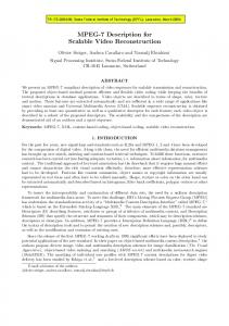
A. Electrical Network Model in the RTS In the proposed HIL setup the electrical lines are threephase (3-ph), modeled with generic unbalanced, PI-line equivalents. Every node is characterized by the presence of a one or multiple 3-ph loads or distributed energy resources (DERs). The active and reactive power profiles can be set in each phase by controlling the absorbed or injected powers, respectively. In the RT network model, this can be achieved by simulating the loads / DERs with controlled current generators connected to each phase. The current references of the generators are acquired using the process that is shown in more detail in Fig. 2.
PROPOSED HIL SETUP FOR THE RTSE PERFORMANCE ASSESSMENT
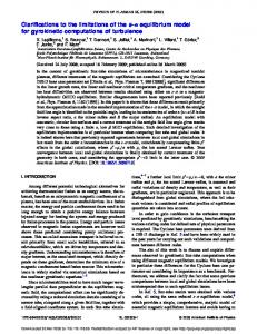
Fig. 1 illustrates the HIL setup that has been designed in the Authors’ laboratory in order to assess the performance of the RTSE. It consists of an RTS that communicates via local Ethernet network with the PDC and the SE. The RTS model includes the electrical network, the sensors and the PMUs. Three-phase bus voltage and injected current signals, representing the true system state, are given as input to the simulated sensors that add noise on top of them and forward them to the PMUs supposed to be installed in some of the network buses. The PMUs estimate the synchrophasors of nodal voltages and injected/absorbed currents, encapsulate them according to the IEEE Std. C37.118.2-2011 [19] and stream the relevant frames through the telecom network to the PDC. The true state needs to be time-stamped using an UTC time reference with the help of an internal dedicated board in the RTS (see [20] for further details). In this respect, the hardware setup that we have adopted is composed by the Opal-RT eMEGAsim RTS equipped with a Spectracom Tsync-PCIe express GPS synchronization module. This synchronization hardware allows to timestamp each quantity in the RTS model in correspondence of each discrete time-step. The dataframes are received by the PDC and, after they are decapsulated, aggregated and time-aligned, are given to a Kalman Filter (KF)-based SE [13]. The PDC together with the SE are also GPS synchronized. Therefore, the estimated state can be compared with the true state coming from the RTS, in order to assess the SE error.
Real%Time)Simulator) 2))Sensors) model)
LabVIEW)
3))PMUs) model)
BUS 1 OS Bemmel
PMU1%
BUS 2 Lingewal
BUS 3 Hoogerbrugge (Elst)
PMU2%
BUS 4 Rijkerswoerdse straat
BUS 5 Loostraat
BUS 6 Waterkant
BUS 7 W.Z.C.
BUS 16 Reigersbos
BUS 13 Dullert
BUS 14 Dullert
BUS 17 Uivernest
BUS 15 Kuunskop
BUS 18 De Zilver
PMUm%
BUS 8 Tuindorp
BUS 9 Het Buiten
BUS 10 Warmoezerij
BUS 11 Blauwenburcht
C37.118)encapsulaBon)
1))Network) model)
4))PDC)
Telecom)
5))KF%SE)
a))C37.118)) decapsulaBon) b))Synchrophasors’) Telecom) aggregaBon) b))Synchrophasors’) Bme%alignment)
Figure 2. Scheme of the controllable nodal absorbed / injected powers.
As stated before, the accuracy of the RTSE requires the knowledge of the true system state (i.e., the voltage phasors in all the buses). If the simulated network has an a-priori fixed frequency, its value (ω/2π) can be expressed as integer multiple of the RTS integration time-step. Therefore, the computation of the true nodal voltage and current phasors (and also the power injections) can be done by assessing the relevant DFT-bin in correspondence of the rated system frequency. So, the real and imaginary part of a generic phasor of a signal u(t) at frequency ω/2π are simply given by:
( ) T Im ( U ) = mean !"u(t)cos(ω t)#$ T Re U = mean !"u(t)sin(ω t)#$
(1)
where T is the period corresponding to the grid rated frequency. B. Sensors Model in the RTS The role of the developed sensors model is to simulate in RT the noise that is added to the true voltage and current signals and, then, forward these noisy quantities to a PMU model also represented inside the RTS [20]. It is important to mention that the discrete-time voltage signals, before forwarded to the simulated sensors, are already affected by a noise, which represents any unwanted distortion of the power signal that cannot be classified as harmonic distortion (e.g. [21], [22]). The so-called "grid noise" may arise from the operation of power electronic devices, control circuits, arcing equipment and switching power supplies. It is a Gaussian random noise with zero-mean and a maximum value equal to 1% of the RMS phase-to-ground voltage magnitude.
BUS 12 Giebesland
True)state)
EsBmated)state)
Error)
Figure 1. The proposed HIL setup for the RTSE performance assessment.
The discrete-time signal (representing a generic 3-ph bus voltages or injected currents) entering in the sensors model and associated to a grid in steady state conditions can be expressed as:
S[n] = A⋅cos(ω nΔt + φ )
(2)
where A and φ are the magnitude and the phase of the main tone of the spectrum, Δt is the RTS integration time-step whereas n is the sample number1.
As an example, Fig. 3a and Fig. 3b show the profiles of the voltage magnitude (in V phase-to-ground RMS) and phase (in radians), respectively, for phase α of bus #3 of the grid shown in Fig. 4 extracted by the PMU implemented in the RTS model.
We assume to represent in the simulated sensor the following sources of errors (e.g., [23], [24]):
Voltage magnitude (phase−to−ground RMS)
5756
§ Gain error: it arises when the actual sensor transformation ratio is not equal to the rated one; § Phase error: it is due to the phase displacement introduced by the sensors2. We also make the following assumptions:
5755
5754
5753
5752
5751
5750
0
50
100
150
200
a)
§ We disregard the limited bandwidth of the sensor;
250 Time−step
300
350
400
450
500
−4
−5.345
§ The sensor non-linearity error is negligible;
x 10
−5.35
Voltage phase (radians)
§ We neglect the cross-talk interferences; § The voltage and current sensors saturate at 120% of the rated voltage and current, respectively. Therefore, the noisy signal in the output of the sensor model can be expressed as:
(
)
S noisy [n] = A + ΔA[n] ⋅cos(ω nΔt + φ + Δφ[n])
−5.355
−5.36
−5.365
−5.37
−5.375
(3)
where ΔA[n] and Δφ [n] are the randomly generated magnitude and phase noises added to each sample n. They are calculated based on the known sensor's accuracy class and their values are random, in the sense that they change from one sample to another. The uncertainties are calculated based on the so-called "Type B" evaluation (e.g., [25], [26]). Therefore, we assume a rectangular/uniform probability distribution with a specified interval equal to [-3σA, +3σA] and [-3σϕ, +3σϕ] for the amplitude and phase, respectively, and a mean value equal to 0. In this case, σA and σϕ are the corresponding standard deviations of the sensors amplitude and phase errors assuming a Gaussian distribution, which is associated to the so-called "Type A" evaluation of the sensors’ uncertainties3.
b)
0
50
100
150
200
250 Time−step
300
350
400
450
500
Figure 3. a) PMU-extracted voltage magnitude (in V phase-to-ground RMS) and b) phase (in radians) of phase α of Bus #3, as a function of time.
C. PMUs model in the RTS In order to simulate properly a PMU inside the RTS and connect it with the devices under test, the following functionalities are needed: (a) a RT implementation of the adopted synchrophasor estimation algorithm; (b) the GPS synchronization and (c) a data streaming module that encapsulates and streams the PMU dataset according to one of the available Standards (for instance IEEE C37.118.2-2011, IEC-61850 etc.). The detailed model of the RTS PMU is described in detail in [20]. D. PDC The PDC collects synchrophasor data and other quantities (i.e., frequency, ROCOF, nodal injected/absorbed powers, After performing simple trigonometric calculations, (3) etc.) that are estimated by the simulated PMUs and then it can be expressed as a sum of four different terms: transmits this information to other applications like simple visualization tools or others that perform even more (4) S noisy [n] = S noisy,1[n]+S noisy,2 [n]+S noisy,3[n]+S noisy,4 [n] sophisticated operations, such as the SE. The adopted PDC has been fully developed by the Authors in LabVIEW. It is Snoisy,1[n] = A⋅ cos(ω nΔt + φ ) ⋅ cos(Δφ [n]) ≈ S[n] able to communicate with the simulated PMUs, it decapsulates the IEEE C.37.118.2011 dataframes and, then, the S[n] Snoisy,2 [n] = ΔA[n]⋅ cos(ω nΔt + φ ) ⋅ cos(Δφ [n]) ≈ ΔA[n]⋅ A (5) synchrophasors are aggregated and time-aligned in a circular buffer, based on the timestamps. Finally, a sub-set of the Snoisy,3[n] = -A⋅ cos(ω nΔt + φ − π 2) ⋅sin(Δφ [n]) measured dataset is forwarded to the SE with the minimum time latency. S [n]: -ΔA[n]⋅ cos(ω nΔt + φ − π 2) ⋅sin(Δφ [n]) ≈ 0. noisy,4
1
The voltage signals, as it has been explained above, are already distorted by the presence of the grid noise. 2 Note that the limits of gain and phase errors imposed by [23], [24] for 0.1class sensors are 10-3 in p.u. and 1.5 ⋅ 10-3 radians, respectively. 3 The interval of the uniform distribution is taken equal to [-3σ, +3σ], based on the tolerance interval of the Gaussian distribution that is equal to 99.7%.
E. Discrete Kalman Filter State Estimator The SE receives the data from the PDC and estimates the system state x ∈ ℝ3(2n) defined as: T
α ,b,c α ,b,c α ,b,c # x = !"V1,rα ,b,c ,…,Vn,r ,V1,im ,…,Vn,im $
(6)
α ,b,c where n is the number of buses and Vi,rα ,b,c , Vi,im are the 3-ph
real and imaginary parts of the voltage at bus i, respectively.
admittance matrix elements, respectively. Therefore, HI is equal to :
! pm G −Bihpm H I = # ih # B pm G pm ih " ih
Before describing the adopted Discrete Kalman Filter (DKF) -SE process, we list here below the relevant hypotheses: § normality of the noise of both the measurements and the process model of the DKF; § the noise distributions of the measurements are independent and identical distributed (IID); § the admittance matrix of the observed grid is known. The adopted DKF-SE algorithm is described by the following set of equations (e.g., [27], [28]):
x k = x k−1 + w k−1
(7)
z k = Hx k + v k
(8)
where: • k is the time-step index; • w ∈ ℝ3(2n) represents the process noise, assumed white and Gaussian, p(w)∼N(0,Q); • z ∈ ℝm represents the set of available measurements; m
• v ∈ ℝ represents the measurement noise, assumed white, Gaussian, independent from w, p(v)∼N(0,R) and composed by IID variables; • H is the matrix that represents the linear link between the measurements and the states, for the case of null measurement noise. The process model of (7) is an autoregressive integrated moving average - ARIMA (0,1,0) and is the one typically proposed for very frequent measurements. It is important to recall that H does not represent a linear approximation of the network model, since it corresponds to the exact link between measurements and states. In this respect, H is equal to: !H $ (9) H =# V& #"H I &% where HV is the part related to the bus voltage measurements, consisting of ones or zeros and directly inferred from (8), whereas HI is the part related to the injected current measurements and can be derived in a straightforward way from the equations that represent the real and imaginary parts of the 3-ph injected current phasors: n
3
m $ I i,rp = ∑∑"#GihpmVh,rm − BihpmVh,im %
(10)
h=1 m=1 n
3
p m I i,im = ∑∑!"GihpmVh,im + BihpmVh,rm #$
(11)
h=1 m=1
where i and h are the bus indices, p and m are the phase indices, and G and B are the real the imaginary parts of the
$ &. & %
(12)
The measurement noise covariance matrix R and the process noise covariance matrix Q can significantly affect the RTSE accuracy as discussed in [8]. R represents the accuracies of the measurement devices, whereas Q is related to uncertainty introduced by the process model to predict the system state. In this paper, we assess Q at every time-step based on the proposed Method #2 presented in [13]. IV.
APPLICATION EXAMPLE AND PERFORMANCE ASSESSMENT
The HIL setup described in Section III has been adopted to test an ADN composed by a real medium voltage feeder of the Alliander electrical distribution grid in the Netherlands. It is shown in Fig. 4. The selected feeder is called BLM 2.10 and it consists of 18 buses. This feeder has been selected since the HIL setup reflects the real installation of sensors/PMUs in this specific distribution system. Therefore, the network parameters, loads, sensors classes and PMU characteristics correspond to the real ones. The voltage of the slack bus (BUS 1 OS Bemmel in Fig. 4) is equal to 10 kV RMS line-to-line. One DER is connected in bus #7 (Bus 7 W.Z.C.). It is a synchronous Combined Heat and Power (CHP) unit that injects a total active power equal to 300 kW (it does not inject any reactive power). The feeding network short-circuit power is equal to Ssc = 300 MVA and the short-circuit ratio Rsc / Xsc = 0.1. The fixed system frequency is equal to 50 Hz. The used voltage and current sensors are assumed to be of class 0.1. The loads are supposed to absorb 25% of the rated power of the transformers with a power factor of 0.98. The PMUs location has been chosen as a function of the following conditions: • installation constraints set by the network operator (i.e., telecommunication bandwidth, physical space to install sensors and PMUs, etc.); • network observability. In this respect, 10 out of 18 network buses are equipped with PMUs, i.e. buses number 1, 3, 5, 6, 8, 10, 12, 13, 15 and 17. A. RTSE Accuracy Assessment In this sub-section, in order to assess the RTSE accuracy, a comparison between the RTSE results and the true state obtained from the RTS is presented. Fig. 5 shows the mean of the absolute errors and the standard deviations of the errors of the voltage magnitude (in p.u.) and phase (in radians) for a time-window of 7 s. These values are assessed for each time frame provided by the PMUs (i.e., 20 ms) and refer to all the network nodal voltages. As it can be observed, magnitude and phase error means and standard deviations are in the order of X⋅10-5 (namely, in the order to tens of parts per million). By considering the
BUS 1 OS Bemmel
Means of the absolute errors
Standard deviations of the errors
−5
Voltage magnitude [p.u.]
realism of the HIL simulation, these results prove the possibility to track with extremely high quality and fidelity the system state of ADNs using the proposed approach, namely a suitable combination of PMUs and DKF-RTSE.
5.4
−5
x 10
7.8
5.3 7.7
5.2 5.1
7.6 5 4.9
7.5
4.8 4.7
BUS 2 Lingewal
0
1
2
3
4
5
7.4
6
Voltage phase [radians]
−5
BUS 3 Hoogerbrugge (Elst)
BUS 4 Rijkerswoerdse straat
7
7.5
1
2
1
2
3
4
5
6
3
4
5
6
x 10
6.5 7 6 6.5
5.5 5
6
4.5 5.5 1
2
3
4
5
6
0
time [s]
BUS 16 Reigersbos
BUS 13 Dullert
0
−5
x 10
0 BUS 5 Loostraat
x 10
time [s]
Figure 5. Mean ans standard deviations of the absolute errors of the voltage magnitude (in p.u.) and phase (in radians) as a function of time. BUS 6 Waterkant
BUS 7 W.Z.C.
BUS 14 Dullert
BUS 17 Uivernest
BUS 15 Kuunskop
BUS 18 De Zilver
Time-stamp of the synchrophasor
Dataset arrives to the PDC
Beginning of the SE
Estimated state available
BUS 8 Tuindorp
time
Δt1 BUS 9 Het Buiten
BUS 10 Warmoezerij
BUS 11 Blauwenburcht
BUS 12 Giebesland
t0
Figure 4. The simulated grid structure composed by the Alliader 10 kV feeder BML 2.10.
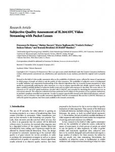
B. RTSE Time Latencies Assessment In order to compute the total and individual time latencies of each step of the RTSE chain, the flow of the data is tagged with UTC-synchronized systems along the whole process. This enables to measure the time that is needed in order to accomplish each of the steps shown in Fig. 6. In particular, as it is shown in Fig. 6, the following absolute time-tags can be recorded:
1
CDF (latency)
§ the instant the SE process is completed t3. Based on these absolute times, it is possible to define the time latencies between two consecutive steps of the process in the following way:
Δti = ti − ti−1 ,
i = 1,…,3
(13)
The total time latency is calculated as:
Δttotal = Δt1 + Δt2 + Δt3 .
Arrival in PDC Beginning of SE End of SE
0.6
= 30.63 ms = 0.28 ms
0.4
= 50.82 ms = 0.27 ms
= 53.61 ms = 0.45 ms
0.2 0
0
10
20
30 latency [ms]
40
50
60
70
Figure 7. CDF of the latencies of each step of the RTSE process together with their mean and stardard deviation values.
V. (14)
t3
Figure 7 shows the latency of the overall process expressed as cumulative distribution functions (CDFs) of time differences as they appear in Fig. 6. As it can be observed, the whole RTSE process is completed within a time of less than 55 ms. This remarkable performance potentially enables the coupling of the RTSE process with new protection and real-time control applications for ADNs.
0.8
§ the time of the SE start t2;
Δt3 t2
Figure 6. Absolute time-tagging of the data flow in the HIL setup.
§ the synchrophasor's time-tag t0; § the time the data arrives to the PDC t1;
Δt2 t1
CONCLUSIONS
We have conducted a performance assessment, in terms of RTSE accuracy and latency using an HIL setup fully developed at the Authors’ laboratory. In the first part of the paper, we have provided a description of the individual
components of the HIL setup, whereas in the second part we have focused on the performance assessment of the RTSE. The validation has been done using a real medium voltage feeder of the Alliander 10 kV electrical distribution grid in the Netherlands. The results concerning the RTSE accuracy show magnitude and phase error means and standard deviations in the order of tens of parts per million. By considering the realism of the HIL simulation, these results prove the possibility to track with extremely high quality and fidelity the system state of ADNs using the proposed approach, namely a suitable combination of PMUs and RTSE. Concerning the latency assessment, the whole RTSE process is completed within a time of less than 55 ms. In summary, we can conclude that the proposed RTSE process is characterized by remarkable accuracy and latency performances that, combined with the high refresh rate of the process, make it suitable to be coupled with new protection and real-time control applications specifically designed for ADNs. ACKNOWLEDGMENT The Authors kindly acknowledge Prof. Lorenzo Peretto for the useful discussion concerning the representation of the uncertainties in the sensor model and Mr. Carl Mugnier, Mr. Chenxi Wu and Mr. Roman Ségur for their contribution in the development of the HIL and software setups.
[11] [12] [13]
[14]
[15]
[16]
[17]
[18]
REFERENCES [1]
N. Jenkins, R. Allan, P. Crossley, D. Kirschen and G. Strbac, Embedded Generation, London, U.K.: Inst. Elect. Eng., 2000. [2] IEEE Guide for Design, Operation, and Integration of Distributed Resource Island Systems with Electric Power Systems, IEEE Std. 1547.4, 2011. [3] IEEE Recommended Practice for Interconnecting Distributed Resources with Electric Power Systems Distribution Secondary Networks, IEEE Std. 1547.6, 2011. [4] IEEE Guide for Smart Grid Interoperability of Energy Technology and Information Technology Operation with the Electric Power System (EPS), End-Use Applications, and Loads, IEEE Std. 2030, 2011. [5] Development and Operation of Active Distribution Networks, Cigré Working Group C6.11, Apr. 2011. [6] K. Christakou, J.-Y. Le Boudec, M. Paolone, and D.-C. Tomozei, "Efficient computation of sensitivity coefficients of node voltages and line currents in unbalanced radial electrical distribution networks," IEEE Trans. on Smart Grid, vol. 4, no. 2, pp. 741– 750, June 2013. [7] A.G. Phadke, and J. S. Thorp, Synchronized Phasor Measurements and Their Applications, New York: Springer, 2008. [8] S. Sarri, M. Paolone, R. Cherkaoui, A. Borghetti, F. Napolitano, and C.A. Nucci, "State estimation of active distribution networks: comparison between WLS and Kalman-Filter algorithms integrating PMUs," presented at the 3rd IEEE PES Inn. Smart Grid Tech. (ISGT) Europe Conf., Berlin, Germany, Oct. 14-17, 2012. [9] IEEE Standard for Synchrophasor Measurements for Power Systems, IEEE Std. C37.118.1, 2011. [10] P. Romano, and M. Paolone, "Enhanced interpolated-DFT for synchrophasor estimation in FPGAs: theory, implementation, and
[19] [20] [21]
[22] [23] [24] [25] [26] [27] [28]
validation of a PMU prototype," IEEE Trans. on Instr. and Meas., vol. 63, no. 12, pp.2824-2836, Dec. 2014. D. A. Haughton, and G. T. Heydt, "A linear state estimation formulation for smart distribution systems," IEEE Trans. on Power Syst., vol. 28, no. 2, pp. 1187-1195, May 2013. K. D. Jones, J. S. Thorp, and R. M. Gardner, "Three-phase linear state estimation with phasor measurements," IEEE PES Gen. Meet., Vancouver, Canada, July 21-25, 2013. L. Zanni, S. Sarri, M. Pignati, R. Cherkaoui, and M. Paolone, "Probabilistic assessment of the process-noise covariance matrix of discrete Kalman Filter state estimation of active distribution networks, " in Proc. Intern. Conf. of Prob. Methods Applied to Power Syst., Durham, UK, July 7-10, 2014. W. Ren, M. Sloderbeck, M. Steurer, V. Dinavahi, T. Noda, S.Filizadeh, A. R. Chevrefils, M. Matar, R. Iravani, C. Dufour, J.Belanger, M.O. Faruque, K. Strunz, and J. A. Martinez, “Interfacing issues in real-time digital simulators,” IEEE Trans. on Power Del., vol. 26, no. 2, pp. 1221-1230, Apr. 2011. G. Valverde, D. Cai, J. Fitch, and V. Terzija, "Enhanced state estimation with real-time updated network parameters using SMT," IEEE PES Gen. Meet., Calgary, Alberta, Canada, July 2630, 2009. D. Ouellette, M. Desjardine, R. Kuffel, Y. Zhang, and E. Xu, "Using a real time digital simulator with phasor measurement unit technology," Advanced Power System Automation and Protection (APAP), 2011 International Conference on, vol. 3, pp. 2472-2476, 16-20 Oct. 2011. D. R. Gurushinghe, A. D. Rajapakse, D. Muthumuni, "Modeling of a synchrophasor measurement units into an electromagnetic transient simulation program," International Conference on Power Systems Transients (ISPT), Vancouver, Canada, July 18-20, 2013. A.T. Al-Hammouri, L. Nordstrom, M. Chenine, L. Vanfretti, N. Honeth, and R. Leelaruji, "Virtualization of synchronized phasor measurement units within real-time simulators for smart grid applications," IEEE PES Gen. Meet., San Diego, CA, 22-26 July 2012. IEEE Standard for Synchrophasor Measurements for Power Systems, IEEE Standard C37.118.2, 2011. P. Romano, M. Pignati and M. Paolone, “Integration of an IEEE Std. C37.118 compliant PMU into a Real-Time Simulator”, Proc. of the 2015 IEEE PowerTech, Eindhoven, June 29 July 2, 2015. E. Scala, "Development and characterization of a distributed measurement system for the evaluation of voltage quality in electric power networks," Ph.D. dissertation, Dept. Elec. Eng., Univ. of Bologna, 2008. IEC 60050-161 International Electrotechnical Vocabulary Electromagnetic Compatibility, International Electrotechnical Commission, Geneva, Switzerland, 1997. IEC 60044-7 International Standard, Instrument Transformers Part 7: Electronic Voltage Transformers, International Electrotechnical Commission, 1999. IEC 60044-8 International Standard, Instrument Transformers Part 8: Electronic Current Transformers, International Electrotechnical Commission, 2002. Evaluation of measurement data - Guide to the expression of uncertainty in measurement, JCGM 100:2008 (GUM 1995 with minor corrections). International vocabulary of metrology - Basic and general concepts and associated terms (VIM), JCGM 200:2008. S. Debs, and R. E. Larson, "A dynamic estimator for tracking the state of a power system, " IEEE Trans. on Power App. and Syst., vol. PAS-89, no. 7, pp. 1670-1678, Sept. 1970. J. Zhang, G. Welch, G.Bishop, and Z. Huang, "A two-stage Kalman Filter approach for robust and real-time power system state estimation, " IEEE Trans. on Sust. Energy, vol. 5, no. 2, pp. 629-636, April 2014.