A Heterogeneous Two-Server Queueing System with ... - APORC

The Eighth International Symposium on Operations Research and Its Applications (ISORA’09) Zhangjiajie, China, September 20–22, 2009 Copyright © 2009 ORSC & APORC, pp. 230–244

A Heterogeneous Two-Server Queueing System with Balking and Server Breakdowns Dequan Yue1 1 Department 2 Department

Wuyi Yue2

Jun Yu1

Ruiling Tian1

of Statistics, College of Science, Yanshan University, Qinhuangdao 066004, China of Intelligence and Informatics, Konan University, Kobe 658-8501, Japan

Abstract In this paper, we study an M/M/2 queueing system with balking and two heterogeneous servers, Server 1 and Server 2. Customers arrive according to a Poisson process and form a single waiting line. Two parallel servers provide heterogeneous exponential service to customers on a firstcome first-served basis. It is assumed that Server 1 is perfectly reliable and Server 2 is subject to breakdowns. For this system, we obtain the stationary condition where the system reaches a steady state. We also obtain the steady-state probabilities in a matrix form by using a matrix-geometric solution method. Finally, we produce explicit expressions of some performance measures such as the mean system size, the average balking rate and the probabilities that Server 2 is in various states. Numerical illustrations are also provided. Keywords Queueing system; balking; breakdowns; matrix-geometric solution; mean system size

1

Introduction

Recent decades have seen an increasing interest in queueing systems with server breakdowns. This has been due to their applications in manufacturing systems, service systems, telecommunications and computer systems. In many practical queueing systems, situations often occur where servers are subject to breakdowns. For example, in a machine processing center, machine breakdowns may occur due to factors such as power failure, lack of preventive maintenance, or the use of inferior row materials. Other examples of queueing systems with server breakdowns can be found in service systems, computer systems and telecommunication systems. Single server queueing systems with server breakdowns have been studied by many researchers including Federgruen and Green [1], Li et al. [2], Tang [3], Nakdimon and Yechiali [4], Wang et al. [5], Wang et al. [6], Choudhury and Tadj [7], to mention a few. Multi-server queueing systems with server breakdowns are more flexible and applicable in practice than single server counterparts. However, due to their analytical complexity, there have been only a few studies carried out on multi-server queueing system with server breakdowns. Mitrany and Avi-Itzhak [8] studied an M/M/N queue with server breakdowns and ample repair capacity. In their study, the moment generating function of the queue size is obtained by using the transformation method. Vinod [9] considered the same model using the matrix-geometric solution method. For N = 1, Vinod [9] imposed some restrictions on the server down-periods (either independent of the queue length or

A Heterogeneous Two-Server Queueing System

231

only occurring when the server is active). Neuts and Lucantoni [10] and Wartenhosrt [11] extended the models studied in [8] and [9] by considering a limited repair capacity. Neuts and Lucantoni [10] considered a single queue of customers, each served by one of N parallel servers. Wartenhosrt [11] considered N single-server queueing stations, each serving its own stream of customers. Wang and Chang [12] studied an M/M/R/N queue with balking, reneging and server breakdowns from the viewpoint of queueing. They solved the steady-state probability equations iteratively and derived the steady-state probabilities in a matrix form. The models mentioned above all assumed the servers to be homogeneous, where the individual service rates were the same for all the servers in the system. This assumption may be valid only when the service process is highly mechanically or electronically controlled. In a queueing system with human servers, we can not expect work to be carried out at the same rate. We face situations of this kind in our everyday life, e.g., at checkout counters in department stores, in banks, in hospitals, etc. Singh [13] studied an M/M/2 queueing system with balking and heterogenous servers. In [13], the author obtained the stationary queue length distribution and the mean queue length and also compared the model with heterogenous servers and the model with homogenous servers. Kumar and Madheswari [14] studied an M/M/2 queueing system with heterogenous servers and multiple vacations by using the matrix-geometric solution method. They studied the stationary queue length distribution and waiting time distribution along with their means via the rate matrix. Yue et al. [15] further considered the model in [14]. They obtained the explicit expression of the rate matrix and proved the conditional stochastic decomposition results for the stationary queue length and waiting time. Madan et al. [16] studied a two-server queue with Bernoulli schedules and a single vacation policy where the two servers provide heterogenous exponential service to customers. They obtained steady-state probability generating functions of the system size for various states of the servers. The models studied in [13]-[16] all assume that the servers are reliable. However, we know that there are many practical queueing situations where the servers are subject to lengthy and unpredictable breakdowns. For example, in a machine processing system, machines may subject to breakdowns during production or when the system is idle. Failures occurred during production may be due to power failure or the use of inferior row materials, while failures occurred when the system is idle may be due to server’s vacations or planed maintenances. Therefore, failures occurred during production may be different from failures when the system is idle. For this, in this paper, we consider a system with unreliable servers by extending the system model presented in [13]. We model the system as an M/M/2 queueing system with balking and two heterogeneous servers, where Server 1 is perfectly reliable but Server 2 is subject to two types of breakdowns, Type 1 breakdowns and Type 2 breakdowns. Type 1 breakdowns occur only in an idle period of Server 2, while Type 2 breakdowns occur only in a working period of Server 2. In our model, the balking probability depends on the states of servers. If an arriving customer finds at least one server is free and available (i.e., Server 1 is free, or Server 1 is busy while Server 2 is free and available), then the customer joins the system. If the customer finds both servers are busy, then the customer joins the system with probability b0 (0 ≤ b0 ≤ 1), and balks with probability 1 − b0 . If the customer finds Server 1 is busy while Server 2 is unavailable, then the customer joins the system with probability b1 (0 ≤ b1 ≤ 1), and

232

The 8th International Symposium on Operations Research and Its Applications

balks with probability 1 − b1 . The rest of the paper is organized as follows. In Section 2, the model description and a quasi-birth-and-death (QBD) model formulation are presented. In Section 3, the stationary condition is derived. The explicit expressions of the steady-state probabilities in the matrix form and some performance measures are obtained. In Section 4, numerical illustrations are provided to highlight the effect of some parameters on the mean system size. Conclusions are given in Section 5.

2

Model Formulation

In this paper, we consider an M/M/2 queueing system with balking and server breakdowns, where the two servers have different service rates.

2.1

Model Assumptions The assumptions of the system model are given as follows:

(a) Arrivals of customers follow a Poisson process with arrival rate λ . Arriving customers form a single waiting line based on the order of their arrivals. (b) There are two servers in the system. Server 1 is perfectly reliable, while Server 2 is subject to two types of breakdowns. Type 1 breakdowns occur only in an idle period of Server 2, while Type 2 breakdowns occur only in a working period of Server 2. It is assumed that Server 2 has an exponentially distributed lifetime with different failure rates α0 (≥ 0) for Type 1 and α (≥ 0) for Type 2, respectively. Whenever Server 2 breaks down, it is immediately repaired by a repairman. The repaired server is as good as a new one. The customer being serviced just before server breakdown needs to be serviced repeatedly and the elapsed service time is not available. The repair times of Server 2 are assumed to follow an another exponential distribution with repair rate β (β ≥ 0). (c) If an arriving customer finds at least one server is free and available (i.e., Server 1 is free, or Server 1 is busy while Server 2 is free and available), then the customer joins the system. If the customer finds both servers are busy, then the customer joins the system with probability b0 (0 ≤ b0 ≤ 1), and balks with probability 1 − b0 . If the customer finds Server 1 is busy while Server 2 is unavailable, then the customer joins the system with probability b1 (0 ≤ b1 ≤ 1), and balks with probability 1 − b1 . (d) If a customer arrives to find both servers free and available, the customer chooses Server 1 with probability p (p ≥ 0) and Server 2 with probability 1 − p. (e) The two servers provide heterogeneous exponential service to customers on a firstcome first-serviced (FCFS) basis with service rates µ1 and µ2 for Server 1 and Server 2, respectively. (f) All stochastic processes involved in the system are independent of each other.

2.2

QBD Process

Let L(t) be the number of customers in the system at time t, and let J(t) be the status of Server 2 at time t, defined as follows: ⎧ ⎨ 0, Server 2 is busy at time t 1, Server 2 is free at time t J(t) = ⎩ 2, Server 2 is broken down at time t.


233

We define the system state by L(t) and J(t). Then {(L(t), J(t)),t ≥ 0} is a Markovian process with a state space Ω as follows: Ω = {(0, 0), (0, 2)} ∪ {(1, j), j = 0, 1, 2} ∪ {(i, j), i ≥ 2, j = 1, 2}. Define the levels 0 , 1 , 2 , ... as the sets of the system states, 0 = {(0, 0), (0, 2)}, 1 = {(1, 0), (1, 1), (1, 2)}, and i = {(i, 1), (i, 2)} if i ≥ 2, where the elements of the sets are arranged in lexicographical order. Using elementary arguments, the process {(L(t), J(t)),t ≥ 0} has a transition rate matrix Q which has a block-tridiagonal structure given by ⎤ ⎡ B 00 B 01 ⎥ ⎢ B 10 B 11 B 12 ⎥ ⎢ ⎥ ⎢ B A A 21 1 0 ⎥ ⎢ ⎥. A A A Q=⎢ 2 1 0 ⎥ ⎢ ⎥ ⎢ A A A 2 1 0 ⎥ ⎢ ⎦ ⎣ ⋅ ⋅ ⋅ ⋅ ⋅ ⋅

Matrix Q is an infinitesimal generator of the Markov process {(L(t), J(t)),t ≥ 0} and is in the format of a quasi-birth-and-death (QBD) process. The sub-matrices A 0 , A 1 , and A 2 are square matrices of order 2, respectively and are given by ] [ ] [ λ b0 0 −(λ b0 + α + µ1 + µ2 ) α A0 = , A1 = , 0 λ b1 β −(λ b1 + β + µ1 ) [ ] µ1 + µ2 0 A2 = . 0 µ1

3

The boundary matrices are defined by [ ] [ α0 λ p λ (1 − p) −(λ + α0 ) B 00 = , B 01 = 0 0 β −(λ + β ) ⎡ −(λ + α0 + µ1 ) 0 α0 B11 = ⎣ 0 −(λ + α + µ2 ) α β 0 −(λ b1 + β + µ1 ) ⎡ ⎤ ⎡ ⎤ [ µ1 0 λ 0 µ2 ⎣ ⎦ ⎣ ⎦ 0 , B 12 = λ , B 21 = B 10 = µ2 0 0 0 µ1 0 λ b1

0 λ ⎤

]

,

⎦,

µ1 0

0 µ1

]

.

Steady-state Analysis

In this section, we first derive the condition for the system to reach a steady state. Then, we derive the steady-state probabilities of the system by using a matrix-geometric solution method. The computations of the rate matrix and the boundary probability vectors are also discussed. We finally derive some performance measures of the system by using the steady-state probabilities.

234

3.1


Stationary Condition

We now derive the condition for the system to reach a steady state. Define matrix A = A 0 + A 1 + A 2 . Then, matrix A can be written as [ ] −α α A= . β −β It is readily known that A is an irreducible generator of a Markov process. Let π = (π0 , π1 ) be a stationary probability vector of this Markov process. Then, π satisfies the linear A = 0 and π0 + π1 = 1. Solving these equations, we have equations: (π0 , π1 )A

π0 =

β α , π1 = . α +β α +β

By Theorem 3.1.1 in [17], the condition π A 0 e < π A 2 e is the necessary and sufficient condition for stability of the QBD process, where e is a column vector of order 2 with all the elements equal to one. After some routine manipulation, the stationary condition turns out to be

ρ=

λ (α b1 + β b0 ) < 1. (α + β )µ1 + β µ2

(1)

Remark. If we let b0 = b1 = b and α = 0 in Eq. (1), then the stationary condition ρ < 1 becomes bλ < µ1 + µ2 , which is the stationary condition obtained by Singh in [13]. When there is no balking, we let b0 = b1 = 1 in Eq. (1), then the stationary condition ρ < 1 becomes

ρ=

λ (α + β ) < 1. (α + β )µ1 + β µ2

This is the stationary condition obtained by Yu et al. in [18].

3.2

Matrix-geometric Solution

Let L and J be the stationary random variables for the number of customers in the system and the status of Server 2. We denote the stationary probability by Pi j = {L = i, J = j} = lim P{L(t) = i, J(t) = j}, (i, j) ∈ Ω t→∞

where i = 1, 2, ..., j = 0, 1, 2. Under the stationary condition ρ < 1, the stationary probability vector P of the generator Q exists. This stationary probability vector P is partitioned P0 , P1 , P2 , ...), where P0 = (P00 , P02 ), P1 = (P10 , P11 , P12 ), and Pi = (Pi0 , Pi2 ) for as P = (P i ≥ 2. Based on the matrix-geometric solution method in [17], the stationary probability vector P is given by P 0 B 00 + P 1 B 10 = 0, P 0 B 01 + P 1 B 11 + P 2 B 21 = 0, A1 + R A 2 ) = 0, P 1 B 12 + P 2 (A i−2

Pi = P2R

,

i = 3, 4, 5, ...

(2) (3) (4) (5)


235

and the normalizing equation P 0 e + P 1 e 1 + P 2 (II − R )−1 e = 1

(6)

where I is an identity matrix of order 2, e 1 is a column vector of order 3 with all the elements equal to one, and R , called the rate matrix, is the minimal non-negative solution with a spectral radius of less than one, of the matrix quadratic equation as follows: R2A2 + RA1 + A0 = 0.

(7)

In order to obtain the rate matrix R , we need to solve Eq. (7). We accomplish this by letting ( ) r11 r12 R= (8) r21 r22 and using the following relation (see [17, p. 83]), R A 2 e = A 0 e , so we get r12 =

λ b0 µ2 − (1 + )r11 , µ1 µ1

r21 =

λ b1 µ1 − r22 µ1 + µ2 µ1 + µ2

(9) (10)

where A 0 , A 1 , A 2 , B 00 , B 01 , B 10 , B 11 , B 12 and B 21 are given in Subsection 2.2. Substituting R into Eq. (7) and using the Eqs. (9) and (10), after some routine manipulations, we get the following equations: 2 r11 + r11 r22 − f0 r11 − f1 r22 + f1 f3 = 0,

(11)

2 r22 + r11 r22 − f0 r22 − f2 r11 + f2 f4 = 0

(12)

where 1 λ b0 + α λ b0 (λ b1 + β ) + , f1 = , µ1 µ1 + µ2 µ1 + µ2 λ b1 λ b0 + α 1 f2 = , f3 = 1 + (λ b0 + β ), f4 = . µ1 µ1 µ 1 + µ2 f0 = 1 +

From Eq. (11), we get r22 =

1 (r2 − f0 r11 + f1 f3 ). f1 − r11 11

(13)

Substituting Eq. (13) into Eq. (12), we get the third-degree equation containing one variable r11 as follows: 3 2 ar11 + br11 + cr11 + d = 0

(14)

236


where a = f1 − f2 , b = f1 ( f3 − 2 f0 ) + f2 ( f4 + 2 f1 ),

c = f1 [ f1 ( f3 − f2 ) − f0 ( f3 − f0 ) − 2 f2 f4 ] , d = f12 [ f3 ( f3 − f0 ) + f2 f4 ] .

The explicit expression of r11 can be obtained by using the root formula of the thirddegree equation. Then, we can obtain r22 from Eq. (13), r12 from Eq. (9) and r21 from Eq. (10). The details are omitted since the exact solution of Eq. (14) obtained by using the root formula method is lengthy and tedious. However, we can calculate the rate matrix R approximately by using the following simple iterative method. We know that, from Eq. (7), we have [ ] R = − A 0 + R 2 A 2 A −1 (15) 1 . Taking the initial value of R = 0 , we can iteratively solve for R and can check the accuracy of this approximation by using the equality R A 2 e = A 0 e . The value of R will converge 2 A−1 since −A 1 and A 0 + R A 2 are positive. Hence, after each iteration, the elements of R will increase monotonically. We compare the two methods of computing matrix R by a numerical example. The comparison results are given in Table 1, where the values of parameters of the system are given as follows: λ = 10, µ1 = 10, µ2 = 15, b0 = 0.9, b1 = 0.4, p = 0.7, β = 18, α0 = 1 and α = 18. Table 1. Comparison between the root formula method and the iterative method. ri j

Iterative method

Root formula

Error

r11

0.2847946242

0.2847946248

r12

0.1880134376

0.1880134381

6 × 10−10

r21

0.0845427109

0.0845427111

r22

0.1886432220

0.1886432222

5 × 10−10 2 × 10−10 2 × 10−10

Table 1 shows that the iterative method for computing the rate matrix is very simple and accurate. The error is within 10−10 . We will use this iterative method to compute the rate matrix for performing numerical experiments in Section 4.

3.3

Boundary Probability Vectors

In order to obtain the stationary boundary probability vectors P 0 , P 1 and P 2 , we need to solve Eqs. (2)-(4) and Eq. (6). To accomplish this, we first prove that the matrix D = B 11 − B 10 B −1 00 B 01 is a invertible matrix, and then derive the reverse of the matrix D . The following lemma will be needed in our proof. Lemma 1. Let E = (ei j ) be a n × n square matrix defined on a real field. If ∣eii ∣ >

i−1

n

j=1

j=i+1

∑ ∣ei j ∣ + ∑

∣ei j ∣, i = 1, 2, ..., n

(16)


237

where the empty summations ∑0j=1 and ∑nj=n+1 are defined to be zero, then E is invertible. Proof. The proof is simple and thus is omitted. The following symbols will be used in the following derivation: x1 =

β , λ + α0 + β

x2 =

α0 , λ + α0 + β

x3 =

λ +β . λ + α0 + β

Lemma 2. The matrix D is invertible and its inverse D −1 is given by ⎞ ⎛ D11 D21 D31 1 ⎝ D12 D22 D32 ⎠ D −1 = D∣ ∣D D13 D23 D33

(17)

where

D11 = x1 µ1 [λ + p(µ2 + α )] − x3 µ2 (1 − p)(λ b1 + β ) + (λ + µ2 + α )(λ b1 + β ), D12 = x1 µ1 p(µ2 + α ) + (x2 µ2 + α )β + x3 µ2 p(λ b1 + β ), D13 = (x1 µ1 p + β )(λ + µ2 + α ) − x3 µ2 β (1 − p), D21 = x1 µ1 (1 − p)(µ1 + α0 ) + x3 µ1 (1 − p)(λ b1 + β ), D22 = x1 µ1 [λ + (1 − p)(µ1 + α0 )] − x2 µ1 β + (λ + µ1 − x3 µ1 p)(λ b1 + β ) + λ α0 b1 , D23 = x1 µ1 (1 − p)(λ + α0 + µ1 ) + x3 µ1 (1 − p)β , D31 = x2 µ1 (λ + µ2 ) − x3 [α µ1 p + α0 µ2 (1 − p)] + α0 (λ + µ2 + α ) + α µ1 , D32 = x2 µ2 (λ + µ1 ) − x3 [α µ1 p + α0 µ2 (1 − p)] + α (λ + µ1 + α0 ) + α0 µ2 , D33 = x2 µ1 µ2 − x3 [(λ + α )pµ1 + (λ + α0 )µ2 (1 − p)] + (λ + α0 )(λ + µ2 α ) + (λ + α )µ1 and the determinant D∣ = −[(λ + α0 ) + (1 − x3 p)µ1 ]D11 + x3 (1 − p)µ1 D12 + (α0 + x2 µ1 )D13 . ∣D Proof. Let di j represent the (i, j)th element of matrix D , i, j = 1, 2, 3. Then, by matrix manipulation, we have d11 = −(λ + α0 ) − (1 − x3 p)µ1 , d12 = x3 (1 − p)µ1 , d13 = α0 + x2 µ1 , d21 = x3 pµ2 , d22 = −(λ + α ) − [1 − x3 (1 − p)]µ2 , d23 = α + x2 µ2 , d31 = β + x1 pµ1 , d32 = x1 (1 − p)µ1 , d33 = −(λ b1 + β ) − x1 µ1 . It is easy to verify that ∣d11 ∣ − (∣d12 ∣ + ∣d13 ∣) = λ > 0, ∣d22 ∣ − (∣d21 ∣ + ∣d23 ∣) = λ > 0, ∣d33 ∣ − (∣d31 ∣ + ∣d32 ∣) = λ b1 > 0.

238


By Lemma 1, D is invertible. It is not difficult to obtain the co-factor Di j of di j and the D∣ of D which are as given in Lemma 2. Thus the inverse D −1 of matrix D determinate ∣D is obtained. Next, we solve Eqs. (2)-(4) and (6). We define the following matrices: ⎞ ⎛ α 0 µ1 (λ + β )µ1 ⎠, α 0 µ2 (18) F 0 = ⎝ (λ + β )µ2 β µ1 (λ + α0 )µ1 ( ) D11 µ2 + D12 µ1 D21 µ2 + D22 µ1 D31 µ2 + D32 µ1 F1 = (19) D13 µ1 D23 µ1 D33 µ1 where Di j , for i, j = 1, 2, 3, is given by Lemma 2. The following Theorem 1 gives the boundary probability vectors P 0 , P 1 and P 2 . Theorem 1. The boundary probability vectors are given by P0 = P2M 0,

(20)

P1 = P2M 1,

(21)

and P 2 is determined by the following equations: { P2 (M M 1 B12 + A1 + R A2 ) = 0 [ ] P 2 M 0 e + M 1 e 1 + (II − R )−1 e = 1

(22)

where

M1 = −

1 F 1, D∣ ∣D

(23)

M0 = −

1 F 1F 0. D∣ λ (λ + α0 + β )∣D

(24)

Proof. Note that B 00 is invertible, and from Eq. (2) we get that P1 B 10 B −1 P 0 = −P 00 .

(25)

Substituting Eq. (25) into Eq. (3), we get B11 − B 10 B −1 P2 B 21 . P 1 (B 00 B 01 ) = −P

(26)

From Lemma 2, we know that D = B 11 − B 10 B −1 00 B 01 is invertible. Thus, Eq. (26) yields that P2 B 21 D −1 . P 1 = −P

(27)

Substituting Eq. (27) into Eq. (25), we get P 0 = P 2 B 21 D −1 B 10 B −1 00 .

(28)


239

After simple manipulations, we have B21 D −1 = − −B

1 F 1, D∣ ∣D

B 21 D −1 B 10 B −1 00 = −

1 F 1F 0. D∣ λ (λ + α0 + β )∣D

(29) (30)

Substitute Eqs. (29) and (30) into Eqs. (27) and (28), we obtain P 0 and P 1 which are given by Eqs. (20) and (21). Substitute Eqs. (20) and (21) into Eqs. (5) and (6), we get Eq. (22). This proves Theorem 1.

3.4

Performance Measures

The boundary probabilities P 0 , P 1 , P 2 and probabilities P i for i ≥ 3 can be used to find the stationary distribution of the number of customers in the system. Let N denote the number of customers in the system at an arbitrary time under the stationary condition. Theorem 2. The stationary distribution of the number of customers in the system is given by P{N = 0} = P 0 e ,

(31)

P{N = 1} = P 1 e 1 ,

(32)

P{N = i} = P 2 R i−2 e , i ≥ 2

(33)

where the boundary probabilities P 0 , P 1 and P 2 are given by Theorem 1 in Subsection 3.3. Proof. Note that P{N = 0} = P00 + P02 = P 0 e , P{N = 1} = P10 + P11 + P12 = p 1 e 1 , we obtain Eqs. (31) and (32). Eq. (33) is obtained by noting that P{N = i} = Pi0 + Pi2 = P i e , i ≥ 2, and using Eq. (5). This proves Theorem 2. Let ε 1 = (1, 0)T and ε 2 = (0, 1)T represent two identity column vectors of order 2, and let δ 1 = (1, 0, 0)T , δ 2 = (0, 1, 0)T and δ 3 = (0, 0, 1)T represent three identity column vectors of order 3. From Theorem 1 and Theorem 2, we can obtain some other performance measures which are given by the following corollary. Since the proof is simple, the details of the proof are omitted. Corollary. (a) The mean system size E[N] is as follows: [ ] E[N] = P 2 M 1 e 1 + (II − R )−1 e + (II − R )−2 e . (34)

240


(b) The mean number E[Nq ] of customers in the queue is as follows: E[Nq ] = P 2 (II − R )−2 e . (c) The average balking rate Br of customers is as follows: } { M1δ 3 . Br = λ P 2 (II − R )−1 [(1 − b0 )ε 1 + (1 − b1 )ε 2 ] + (1 − b1 )M

(35)

(36)

(d) The probability Pf that Server 2 is free is given by

M0ε 1 + M 1δ 1) . Pf = P 2 (M (e) The probability Pb that Server 2 is busy is given by [ ] Pb = P 2 M 1 δ 2 + (II − R )−1 ε 1 .

(f) The probability Pd that Server 2 is broken down is given by [ ] Pd = P 2 M 0 ε 2 + M 1 δ 3 + (II − R )−1 ε 2 .

4

(37)

(38)

(39)

Numerical Illustrations

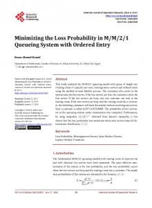
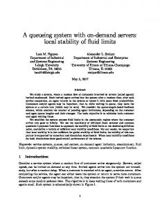
In order to explore the effect of various system parameters on the mean system size, some numerical experiments are performed and the results are displayed by graphs. MATLAB software was used to develop the computer program. In Figs. 1-3, the mean system size E[N] is plotted against the arrival rate λ for chosen values of the service rates µ1 , µ2 , the failure rates α0 , α , and with the joining probabilities b0 , b1 satisfying the stationary condition ρ < 1. In Fig. 1, we fix b0 = 0.9, b1 = 0.5, α0 = 6, α = 8, β = 10, and p = 0.7. The mean system size E[N] is plotted against the arrival rate λ for chosen values of µ1 and µ2 . Figure 1 shows that the mean system size for the case of µ1 = 15 and µ2 = 15 is the smallest among all five cases. This is because that the total service rate µ1 + µ2 = 30 for this case is the largest among all five cases. We observed from Fig. 1 that the mean system size for the case of µ1 = 5 and µ2 = 15 is much larger than that for the case of µ1 = 15 and µ2 = 5 although the total service rate for each of the two cases is the same µ1 + µ2 = 20. This is because when a customer arrives to find both servers free and available, the customer chooses the faster server, Server 2, in the first case with probability 0.3 and the faster server, Server 1, in the second case with probability 0.7. This is why the mean system size for the first case is larger than that for the second case. As expected, the mean system size increases with the increasing of the arrival rate λ , while it decreases with the increasing of the service rate µ1 or µ2 for each server. In Fig. 2, we fix µ1 = 15, µ2 = 10, α0 = 6, α = 8, β = 10, and p = 0.7. The mean system size E[N] is plotted against the arrival rate λ for chosen values of b0 and b1 . Figure 2 shows that the mean system size increases with the increasing of the joining probability b0 or b1 . This is because the larger the probability b0 or b1 is, the more customers are allowed to join the system, which results in the increasing of the mean system size. The graphs of the five cases indicate that the differences in the mean system size steadily


241

8 µ1=5,µ2=15 µ1=10,µ2=15

7

µ1=15,µ2=15 µ1=15,µ2=10

Mean system size Ls

6

µ1=15,µ2=5

5 4 3 2 1 0

2

4

6

8 10 Arrival rate λ

12

14

16

Figure 1: Mean system size E[N] versus arrival rate λ for different values of µ1 and µ2 .

4.0

3.5

Mean system size Ls

3.0

2.5

2.0

1.5 b0=0.3,b1=0.9

1.0

b0=0.6,b1=0.9 b0=0.9,b1=0.9

0.5

b0=0.9,b1=0.6 b0=0.9,b1=0.3

0

2

4

6


12

14

16

Figure 2: Mean system size E[N] versus arrival rate λ for different values of b0 and b1 .

242


decreases with a decreasing arrival rate. This can be explained by noting the fact that for most of the time when the servers are free, the arrival rate is much less than the service rate. Therefore, the mean system size will be very small when the arrival rate is small enough, which results in a decrease in the differences among the mean system sizes for decreasing arrival rates. 3.0

Mean system size Ls

2.5

2.0

1.5

α0=6,α=18

1.0

α0=12,α=18 α0=18,α=18

0.5

α0=18,α=12 α0=18,α=6

0

2

4

6


12

14

16

Figure 3: Mean system size E[N] versus arrival rate λ for different values of α0 and α . In Fig. 3, we fix µ1 = 15, µ2 = 10, b0 = 0.9, b1 = 0.5, β = 10, and p = 0.7. The mean system size E[N] is plotted against the arrival rate λ for chosen values of α0 and α . It is observed from Fig. 3 that the mean system size increases with the increasing of the failure rate α0 and decreases with the increasing of the failure rate α . This can be explained by noting the fact that α0 and α are the different failure rates for Server 2 in its idle time and its busy time, respectively. On one hand, in the busy time of Server 2, the larger the failure rate α is, the smaller the availability of Server 2 is. This results in an increase in the mean system size. On the other hand, the more customers balk (are not allowed to join the system) the more the mean system size increases. This results in a decreasing mean system size. When the increasing mean system size due to the increasing failure rate α is less than the decreasing mean system size due to the balking of customers, the mean system size will decrease as the failure rate α increases. However, this is not so for the case of failure rate α0 . In the idle time of Server 2, the larger the failure rate α0 is, the smaller the availability of Server 2 is. Also, the arriving customers will not balk, since there is at least one free and available server in the idle time of Server 2. This results in an increase in the mean system size. This is why the mean system size increases as the failure rate α0 increases.


5

243

Conclusions

In this paper, a heterogeneous two-server queueing system with balking and server breakdowns was studied. We extended the model in [13] by considering server breakdowns. The model investigated in this paper is more realistic for modeling queueing situations where the server may experience many types of breakdowns which can be realized in manufacturing or production systems. The matrix-geometric solution method has been used in this paper for obtaining the stationary condition and some performance measures such as the stationary distribution of the number of customers in the system and the mean system size. We finally performed numerical experiments to explore the effect of various system parameters on the mean system size.

Acknowledgements This work was supported in part by the National Natural Science Foundation of China (No. 70671088), and was supported in part by GRANT-IN-AID FOR SCIENCE RESEARCH (No. 21500086) and the Hirao Taro Foundation of KUAAR, Japan.

References [1] A. Federgruen and L. Green, Queueing systems with service interruptions, Operations Research, 34 (1986), 752-768. [2] W. Li, D. Shi and X. Chao, Reliability analysis of M/G/1 queueing systems with server breakdowns and vacations, Journal of Applied Probability, 34 (1997), 546-555. [3] Y. Tang, Single-server M/G/1 queueing system subject to breakdowns -some reliability and queueing problems, Microelectronics Reliability, 37 (1997), 315-321. [4] O. Nakdimon and U. Yechiali, Polling systems with breakdowns and repairs, European Journal of Operational Research, 149 (2003), 588-613. [5] K. Wang, T. Wang and W. Pearn, Optimal control of the N policy M/G/1 queueing system with server breakdowns and general startup times, Applied Mathematical Modelling, 31 (2007), 2199-2212. [6] J. Wang, B. Liu and J. Li, Transient analysis of an M/G/1 retrial queue subject to disasters and server failures, European Journal of Operational Research, 189 (2008), 1118-1132. [7] G. Choudhury and L. Tadj, An M/G/1 queue with two phases of service subject to the server breakdown and delayed repair, Applied Mathematical Modelling, 33 (2009), 2699-2709. [8] I. L. Mitrany and B. Avi-Itzhak, A many-server queue with service interruptions, Operations Research, 16 (1968), 628-638. [9] B. Vinod, Unreliable queueing systems, Computers and Operations Research, 12 (1985), 322340. [10] M. F. Neuts and D. M. Lucantoni, A Markovian queue with N servers subject to breakdowns and repairs, Management Science, 25 (1979), 849-861. [11] P. Wartenhosrt, N parallel queueing systems with server breakdown and repair, European Jopurnal of Operational Research, 82 (1995), 302-322. [12] K. H. Wang and Y. C. Chang, Cost analysis of a finite M/M/R queueing system with balking, reneging and server breakdowns, Mathematical Methods of Operations Research, 56 (2002), 169-180. [13] V. P. Singh, Two-server Markovian queues with balking: heterogeneous vs. homogeneous servers, Operations Research, 18 (1970), 145-159.

244


[14] B. K. Kumar and S. P. Madheswari, An M/M/2 queueing system with heterogeneous servers and multiple vacations, Mathematical and Computer Modelling, 41 (2005), 1415-1429. [15] D. Yue, J. Yu and W. Yue, A Markovian queue with two heterogeneous servers and multiple vacations, Journal of Industrial and Management Optimization, 5 (2009), 453-465. [16] K. C. Mandan, W. Abu-Dayyeh and F. Taiyyan, A two server queue with Bernoulli schedules and a single vacation policy, Applied Mathematics and Computation, 145 (2003), 59-71. [17] M. F. Neuts, Matrix-Geometric Solutions in Stochastic Models: An Algorithmic Approach, Baltimore, MD: Johns Hopkins University Press, 1981. [18] J. Yu, D. Yue and R. Tian, Matrix-geometric solution of a repairable queueing system with two heterogeneous servers, Acta Mathematicae Applicate Sinica (in Chinese), 31 (2008), 894-900.