Mathematical and Computer Modelling 41 (2005) 1415-1429 ... computer maintenance and testing, preventive maintenance jobs in a production system, priority.
Availableonlineat www.sciencedirect.com SCIENCE C~DIRECT" ELSEVIER
MATHEMATICAL AND COMPUTER MODELLING
Mathematical and Computer Modelling 41 (2005) 1415-1429 www.elsevier.com/locate/mcm
An M/M/2 Queueing System with Heterogeneous Servers and Multiple Vacations B. K R I S H N A K U M A R AND S. PAVAI M A D H E S W A R I Department of Mathematics Anna University Chennai-600 025, India
(Received February 2004; revised and accepted February 2005) A b s t r a c t - - I n this paper, a Markovian queue with two heterogeneous servers and multiple vacations has been studied. For this system, the stationary queue length distribution and mean system size have been obtained by using matrix geometric method. The busy period analysis of the system and mean waiting time distribution are discussed. Extensive numerical illustrations are provided. @ 2005 Elsevier Ltd. All rights reserved.
Keywords--Heterogeneous time.
servers, Multiple vacations, System size, Busy period, Mean waiting
1. I N T R O D U C T I O N The significant developments in queueing models with server vacation have led to a new branch of queueing systems, namely, "vacation queueing systems". Server vacations may be due to lack of work, server failure, or another task being assigned to the server, which occur in applications like computer maintenance and testing, preventive maintenance jobs in a production system, priority queues, etc. (see [1]). In these systems, the server is not always available to serve its primary customers. In queueing models, vacations can be classified as single server or multiple server involving single vacation or multiple vacations. The server may take a vacation at a random time, after serving at most K customers (K-limited) or after all the customers in the queue are served (exhaustive). Also, depending on the applications, when the server finishes a vacation and there is no customer to be served, the server may take another vacation (multiple vacation model) or it may wait, ready to serve, until a customer arrives (single vacation model). The queueing systems with single or multiple vacation have been introduced by Levy and Yechiali [2]. The literature about vacation models is growing rapidly which includes survey papers by Teghem [3], Doshi [1,4] and the monograph by Takagi [5]. The authors t h a n k the referees for their several constructive comments and suggestions which helped in bringing the paper in its present form. 0895-7177/05/$ - see front matter @ 2005 Elsevier Ltd. All rights reserved. doi:10.1016/j.mcm.2005.02.002
Typeset by .AJMS-TEX
1416
B. KR[SHNA KUMAR AND S. PAVAI MaDHESWARI
The study on multiserver queueing systems generally assumes the servers to be homogeneous in which the individual service rates are the same for all the servers in the system. This assumption may be valid only when the service process is mechanically or electronically controlled. In a queueing system with human servers, the above assumption can hardly be realized. It is common to observe server rendering service to identical jobs at different service rates. This reality leads to modelling such multiserver queueing systems with heterogeneous servers, i.e., the service time distributions may be different for different servers. As noted earlier, the study of vacation queueing systems incorporate the secondary jobs in the modelling. The analysis of queueing systems with heterogeneous servers and servers' vacations help to study the impact of secondary jobs on the determination of system performance. Multiserver queues with servers vacation have been analyzed by a number of authors. Levy and Yechiali [6] have discussed the vacation policy in a multiserver Markovian queue. They have considered a model with 's' homogeneous servers and exponentially distributed vacation times. Using partial generating function technique, the system size has been obtained. Kao and Narayanan [7] have discussed the M/M/s queue with multiple vacations of the servers using a matrix-geometric approach. Gray et al. [8] have discussed a single counter queueing model involving multiple servers with multiple vacations. Recently, an M / M / s queue with multiple vacation and I-limited service has been studied by Tyagi et al. [9]. In literature, there are few other M/M/s vacation queueing models that have been discussed. Mitrany and Avi-Itzhak [10] and Neuts and Lucantoni [11] have analyzed the M / M / s queueing systems where the servers are subject to random breakdowns and repairs. Neuts and Takahashi [12] have pointed out that for the queueing systems with more than two heterogeneous servers, analytical results are intractable and one may have to use algorithmic approach to study even the asymtotic behaviour of the performance measures like stationary distribution of system size and tail probability of waiting time of a customer in the system. Based on this observation, we confine to the study of a two-heterogeneous server Markovian queue with server dependant vacations in this paper. This type of study can be used in real and practical situations. For instance, in machine repairman problems with two heterogeneous servers (the machines), the secondary jobs like maintenance of machine parts depends on the type of machine, which leads to the consideration of two different types of vacation time distribution. The impact of secondary jobs on the system performance measures helps to understand and plan more realistically a real situation than the case without giving due consideration to the secondary jobs. The rest of the paper is organized as follows. In Section 2, the mathematical model is described. Using matrix geometric method, the rate matrix R is found, using which the stationary queue length distribution, mean system size and performance measures are computed. The busy period analysis for the model under consideration is discussed in Section 3. Section 4 studies the waiting time distribution and the corresponding mean. Finally, some numerical results and analysis of algorithmic development have been illustrated in Section 5. 2. M O D E L
DESCRIPTION
Consider an M/M/2 vacation queueing system where the service rate of the servers are not identical. Arrivals of customers follow a Poisson process with parameter ~. Arriving customers form a single waiting line based on the order of their arrivals. The total number of potential customers and the system capacity are assumed to be infinite. There are two exponential servers with service rates >1 and >2 (t'1 ~ #2) for Server 1 and Server 2, respectively. At the end of a vacation period, service commences if a customer is present in the queue. Otherwise, the server takes another vacation immediately and continues in the same manner until it finds at least one customer waiting upon returning from a vacation (multiple vacations). This process holds good for both Servers 1 and 2.
M/M/2 Queueing System
1417
The length of vacation times {Vk,r, r = 1, 2, 3 , . . . } are assumed to be independent and identically distributed exponential random variables with parameters Ok for k = 1, 2 and is independent of the length of the service times and arrival process. The arriving customers are served under the first-come, first-served (FCFS) discipline. The vacation queueing model with heterogeneous server under consideration can be formulated as a continuous time Markov chain (CTMC). The possible states of the system at any epoch are represented by a doublet (i,j) where i > 0 denotes the number of customers in the system and j = 0, 1, 2, 3 denotes the status of the servers. That is, the state (i, 0) represents i (2 0) customers are in the system and both servers are on vacation; the state (i, 1) corresponds to i (_> 1) customers are in the system and Server 1 is busy in the system while Server 2 is on vacation; the state (i, 2) denotes i (> 1) customers are in the system and Server 2 is busy in the system while Server 1 is on vacation; the state (i, 3) indicates that i (_> 2) customers are in the system and both Servers 1 and 2 are busy in the system. We define the levels 0,1,2,... as the set of states 0 = {(0, 0)}, 1 = {(1, 0), (1, 1), (1, 2)} and i = {(i, 0), (i, 1), (i, 2), (i, 3)} if i > 2, where the elements of the sets are arranged in lexieographical order. Using elementary arguments, the infinite-state Markov chain for the model under study has a transition rate matrix Q which has a block-tridiagonal structure given by "Boo Blo
Bol Bll B21
Q=
B12 A1 A2
A0 A1 A2
Ao AI A2
Ao A1
Ao
Matrix Q is an infinitesimal generator of the CTMC and is in the format of a quasi-birthand-death (QBD) process. The submatriees A0, A1, and A2 are of order 4 x 4 and are given by Ao = AI, where I is an identity matrix,
F -(/~ -[- 01 + 02)
&=[!
01
-(~+~1+02)00
02 0 -(A + #2 + 0i)
0 02 0i
o
-(A + ~ + ~2)
and A2 = diag (0, #1, #2, #z + #2). The boundary matrices are defined by Boo = -A, B01 = (A, 0, 0), B10 = (0, #1, ~2) T
Bll =
B12 =
1
--(A @ 01 "~-02) 0
01 -(A @/~1)
02 0
o
o
-(), + ~,2)
A 0 0 A
1
,
and
B21 =
] ,
li oo ~1 0 ~2
We now derive the condition for the system to reach steady state. define matrix A = A0 + AI ÷ A2. Then, matrix A can be written as
--(01+02) A=
0 0 0
01 -02 0 0
02 0 -01 0
0 0~ 01 0
0 #2 #1 To accomplish
this, we
1418
B. KRISHNA KUMAR AND S. PAVAI MADHESWARI
Clearly, the CTMC with generator A is reducible with absorbing state (3,3) and stationary probability vector II = (0, 0, 0, 1). It is well known [13, p. 155] that the standard drift condition HAoe < IIA2e is the necessary and sufficient condition for stability of QBD process where e denotes a column vector with all its elements equal to one. After some routine manipulation, the stability condition turns out to be
< ~ + ~2.
(2.1)
Under the stability condition (2.1), the stationary probability vector X of the generator Q exists. This stationary probability vector X, partitioned as X = (x0, x l , x 2 , . . . ), is given by xoBoo + x l B l o = 0,
(2.2)
xoBm + xlB11 + x2B21 = 0,
(2.3)
xlB12 + x2 (A1 + RA2) = O,
(2.4)
Xi
=
X2R
i--2
,
i = 3~ 4, 5 , . . . ,
(2.~)
R ) - l e = 1,
(2.6)
and the normalizing equation, xo + x l e + x 2 ( I -
where x0 is the probability that no customer is in the system and both servers are on vacation, the vectors x l = (xl0, Xll, x12) and xi = (xi0, x~l, xi2, x~3) for i > 2 are probabilities for i customers in the system in which xij refers to the joint probability that there are i customers in the system and j = 0, 1, 2, 3 corresponds to the status of the servers in the system, I is the identity matrix of order 4 and the matrix R is the minimal nonnegative solution with spectral radius less than one, of the matrix quadratic equation, R2A2 + RA1 + Ao = O,
(2.7)
(see [14, p. 82-83]). Since the square matrices A0, A1, and A2 of order 4 x 4 are upper triangular, R is also a 4 x 4 upper triangular matrix and is obtained from the above quadratic equation and the following relation, RA2e = Aoe. (2.8) The above equation implies that the rate of transition from a state where there are i customers, to a state with i + 1, matches the transition rate from i to i - 1. To obtain R, we know that, from (2.7), R = -AoA-~ 1 - R2A2A-~ 1. Taking the initial value of R = 0, we can iteratively solve for R and can check the accuracy of this approximation by using equation (2.8). The value of R will converge since -A~ -1 and (A0 + R2A2) are positive. Hence, after each iteration, the elements of R will increase monotonically. The boundary probabilities x0, x l , x2, and the probabilities xl for i > 3 can be obtained from (2.2) to (2.6). These steady state joint probabilities are then used to find the mean and the variance of the number of customers in the system and mean waiting time. Let N denote the stationary queue length at an arbitrary time. Therefore, the mean and second moment of the number of customers in the system can be obtained exactly as E ( N ) = Xxe + 2x2c + x2R [ ( I - R) -~ + 2 ( I - R) -1] e
(2.9)
and E ( N 2) -- x l e + 4 x 2 e - x2 [(I - R) -1 + (I - n ) -2 + 2 ( I - R) -~ - 4I] e,
(2.10)
M/M/2 Queueing System
1419
where the column vectors e are of the appropriate dimensions with all elements equal to 1. The variance of the system size can be found. Further, the mean number of customers E(Nj) and the probability distribution I-ij of the number of busy servers in the system are given by
E(M) :
nznj n=k
and
Ilj=~x,~j,
wherek=
n=k
0,
for j = 0 ,
1,
forj=l,2,
2,
for j = 3 ,
and j = 0 corresponds to the case when both servers are on vacation, j = 1, 2 corresponds to the sever-j being busy and the other server on vacation and j = 3 corresponds to the case when both servers are busy. 3. T H E
BUSY
PERIOD
For the vacation model with heterogeneous servers, the busy period is defined to be the interval between the arrival of a customer to an empty system and first epoch thereafter when the system becomes empty again. Therefore, the busy period is the first passage time from state (1,0) to state (0,0). For the vacation model, each busy period starts with a server vacation period in which both Server 1 and Server 2 are on vacation and is followed by a server busy period in which at least one server is busy. The vacation period of the servers is the first passage time from the state (1, 0) to states in the set E = {(i, 1), (i, 2); i > 1}. An idle period begins when a customer completes his service with no customer waiting for service and it ends when the next customer arrives. The length of an idle period is clearly exponentially distributed with parameter A. It is noted that during an idle period both Server 1 and Server 2 are oll vacation. In fact, during a server busy period, if Server 1 is busy, Server 2 can be on vacation or busy and vice versa. However, the definition of a server vacation period does not include these intervals. In order to discuss busy period analysis, the notion of fundamental period (see [14, p. 95-107]) should be briefly reviewed. For the QBD process described above, starting from a state in level i, where i > 3, the first passage time to a state in level i - 1 constitutes a fundamental period. Owing to the structure of the QBD process, the first passage time distribution is invariant in i. Let Gjj,(k, t) denote the conditional probability that a QBD process, starting in the state (i, j) at time t = 0, the first visit to level i - 1 occurs no later than time t, into the state (i - 1,j') and exactly k transitions occur to the left during the first passage time. For convenience, define the joint transforms, oo
Gjj,(z,s)=EZkfo
e-StdGjj,(k,t),
for Izl__0,
(3.1)
k=l
and the matrix G(z, s) = {Gjj, (z, s)}. The matrix G(z, s) is the unique solution to the nonlinear equation, (z, s) = z (sI - A1) -1 A2 + (sI - A1) -1 A0G 2 (z, s), (3.2) (see [14, p. 97]). To discuss the boundary conditions for the vacation model, for i = 1, 2, let (i,i--1) Gjj, (k, t) denote the conditional probability that a QBD process, starting in the state (i, j) at
time 0, reaches the level i - 1 for the first time no later than t, after exactly k transitions to the left and does so by entering the state ( i - 1,j'). Let G(i#-l)(z, s) denote the transform matrix
1420
B. KRISHNA
KUMAR
AND S. PAVAI MADHESWARI
corresponding to G(i,i-t)(k, t). Using arguments similar to that yielding (3.2), we get 6 (2'1) (z, s) = z ( s f -
A1) -1 B21 +
(sl -
A1) -i A0G (z, s) d (2'1) (z, s),
0 (1'0) (z, S) = Z (8ir -- Bll) -1/~10 + (Sir -- Bll) -1B120 (2'1) (z, s) 6 (1'°) (z, s),
(3.3)
d(°'°) (z,s) = [ s---~' ~ 0, 0 ] d0,0) (z, s), where 6 (°,°)(z, s) is the joint transform of the recurrence time to state (0, 0) with at least one visit to a state other than state (0, 0). Note that ~(1, O)(z, s) is of order 3 x 1. The LaplaceStieltjes transform (LST) for the length of a busy period is then given by the first element of d(1, 0)(1+, s), i.e., the element corresponds to the first passage from state (1, 0) to state (0, 0). The busy cycle comprises an idle period and a busy period. The LST for the length of a busy cycle is given by ~(0, 0)(1+, s). Let G = G ( 1 - , 0+), G21 = d (2' 1)(1-, 0+), GlO = d (1' o)(1-, 0+), Goo = d (°'°) ( 1 - , 0+). The positive recurrence of the process Q implies that G, G21, Glo, and Goo are all stochastic and Goo = (1, 1, 1) T. Let Co = ( - A 1 ) - l A 2 , 6"2 = ( - A i ) - l A o . In [14], it has been proved that G is the minimal nonnegative solution to the equation G = Co + C2G 2. By simple algebra, we have formulas for Gij as G21 = -- (A1 + AoG) -1B21,
(3.4)
G10 = - (Bll + B12G21) -1 BlO.
(3.5)
However, when _R is found, we can use the following result due to [15], G = -- (A1 + RA2) -1 A2.
(3.6)
The moments of the various components of a busy cycle are computed in the following manner. Let M1 = ( ° G ( z , s))z=l,s=o. It has been proved in [14 p. 102-103] that the matrix M1 can be computed by successive substitutions in
M1 = -A-11G + C2 (GM1 + M I G ) ,
(3.7)
starting with M1 = O. For the boundary states, differentiating (3.3) with respect to s and setting s = 0, z = 1, yields M21 = - (A1 + AoG) -1 ([ + AoM1) G21, Mlo = - (Bll + B12G21) -1 (I + B12M21) Glo.
(3.8)
It is clear that Mlo can be computed recursively starting with M1 in decreasing order. Denoting Moo as the mean recurrence time for state (0, 0), a similar operation leads to Moo =
Ex,O,O 1 ] G10+[1,0,0]M10.
It is noted that the mean length of a busy cycle is Moo. The first element of the column vector Mlo yields the mean length of a busy period, E(B). The mean length of a server vacation period, E ( 7 ) is 1/(01 + 02). The mean length of a server busy period E(Bs) is then obtained as E(Bs) = E(B) - E(V). Therefore, the fraction of time both Server 1 and Server 2 are on vacation is (E(V) + (1/A))/Moo. This fraction is the same as the probability that both servers are on vacation, as shown in Section 2.
M/M/2 Queueing System
4. W A I T I N G
TIME
1421
ANALYSIS
Let W(.) be the distribution function for the waiting time in the queue of an arriving (tagged) customer. For the multiple vacation model under consideration, we have W ( 0 + ) = 0 because an arrival must either wait for a service completion or a vacation termination of servers. States corresponding to the number of customers present in the system are {0, 1, 2 , . . . } and an absorbing state {*} form the state space of the CTMC. Thus, the state space of the CTMC is {*} U {0, 1, 2 , . . . }. On entering the absorbing state denoted by *, a tagged customer starts receiving service. This happens at the arrival of either Server 1 or Server 2 after vacation when the customer is at the head of the queue. The transition rate matrix Q1 for this absorbing Markov chain is given by * 0 1 2 3 4
QI=
0 1 2 3
co Cl c2
Do B10 0
D1 B21
D A2
4 5
D As
D A2
D
where co = 01 + 0 5 , Do = - c o , Cl ~- [0, ]-tl -~ 02,]-t2 -~- 01] T, c2 = [0,0,0,~tl --~-~2] T,
B l o = [ 0 , 0 , 0 ] T,
D1 =
B2o=
0
#1 0 0
and
0
- ( # 1 + 02)
0
0
0
- ( ~ + 01)
.
The matrix D is 4 x 4 with D = A1 + AI and the matrices A1 and A2 are also 4 x 4 as defined in Section 2. Here, I is an identity matrix of order 4. It is observed that ci, i = 0, 1, 2 gives the rate at which the tagged customer enters the absorbing state. This happens only when the number of customers ahead of the tagged customer is equal to the number of servers at the queue and either Server 1 or Server 2 arrives after completing vacation. Matrices D1 and D imply the rate at which either Server 1 or Server 2 arrives at the queue from the vacation, and hence, the customers ahead of the tagged customer start receiving service. Matrices B20 and A2 give the rate at which customers depart from the system after their service completion. In matrix Q1, the customer arrival rate A is not required since we are considering a FCFS queue discipline and hence, customers that arrive after the tagged customer do not have any impact on the analysis of waiting time. To obtain the mean waiting time, a method used by Kao and Narayanan [7] and Neuts and Lucantoni [11] is applied with appropriate modifications as required in the model under study. The basic intent is to find the time it takes for the tagged customer to reach the absorbing state (*). Define Y(t) = (y. (t), yo (t), Yl (t)~ Y2 ( t ) , . . . ) , where Yi(t) = (yio (t), Yil (t), Y~2(t), yi3 (t)) T , when i > 2, yo(t) is of order 1 x I and y l ( t ) = (ylo(t), y n ( t ) , y12(t)) T and its elements denote the probabilities that at time t the CTMC with generator Q1 is in the respective states of level i. Clearly, y.(t) is the probability that the tagged customer is in the absorbing state at time t. Because
1422
B. KRISHNA
KUMAR
AND S. PAVAI MADHESWARI
of the memoryless property of the Poisson arrival process, at time 0, Y(0) = {0, x0, xl, x 2 , . . . } where x0 and xi are the steady state probabilities of the CTMC with generator Q obtained in Section 2. It is seen that the waiting time distribution W ( t ) = y, (t) for t _> 0. In finding the waiting time distribution, it is assumed that the process starts with initial probability Y(0). The differential equation Y ' ( t ) = Y ( t ) Q 1 for t _> 0 reduces to 2
i=0
(4.1)
vo' (t) = y0 (t) Do + Yl (t) B10, Yl' (t) = Yl (t) D1 ÷ Y2 (t)/320, i = 2, 3 , 4 , . . . .
yi t (t) = Yi (t) D 4- Yi+l (t) A2,
The tagged customer finds the system in state (i, j) with probability Yi,j(O) for i > 2, the LST of the first passage time to a state ( 2 , f ) in level 2 is given by the fth element of the row vector ¢(s). As in [11], we have c~
i-2
(4.2) i=2
Let Cj (i, s) be the LST of the absorbing time to state * given that the process starts from state (i,j) of the levels 0, 1, 2. Let ~(i, s) denote the column vector containing Cj(i, s). On the basis of Q1, we can write the following relations, (0, s) = (sI - Do) -1 c0,
(1, s)
= (sI - D1) -1
(4.3)
B10~ (0, s)
4- ( s I -
D1) -1 cl,
(2, s) = (sI - D2) -1 B2o~I, (1, s) 4- (sI - D) -1 c2.
(4.4) (4.5)
It can be seen that the LST for the waiting time distribution is given by 1
IY (s) = E
Yi (0) ~5 (i, s) ÷ ¢ (s) • (2, s).
(4.6)
i=0
4.1. M e a n Waiting T i m e The mean waiting time can be obtained from l~(s), 1
E (W) = - E y i
(0) aS' (i, 0) - ¢ ' (0) e - 9 (0) ~' (2,0).
(4.7)
i=0
The first term gives the mean time to reach an absorbing state by the tagged customer if the system is either at level 0 or 1 on its arrival; the second and third terms give the time to reach the absorbing state * if the system is in level _> 2 on the arrival of a tagged customer. To obtain the mean waiting time, we must calculate the value of each term in equation (4.7). Differentiating (4.3) with respect to s and setting s = 0, we have 1 - ~ ' (0,0) = 01 + 02'
(4.8)
Similarly, differentiating (4.4) and (4.5) with respect to s and at s = 0, we get
-d)' (I, 0)
=
(-DI) -2 el
(4.9)
M/M/2 Queueing System and
(2,0) = (-D) -I [e +
1423
B2o(-D)-2ci],
(4.10)
where we have used the relation B2oe + De + c2 = 0 and (4.9). Thus, we can find {I)'(i, 0) recursively. As yi(0) = xl, and using (4.8)-(4.10), we compute the first term of equation (4.7). The expression •(0) = y2~i22yi(0)U i-2, where U = ( - D ) - I A 2 , is obtained by substitut1 ing s = 0 in (4.2). It is noted that ~b(0)e = 1 - Y2~=0 xle, since Ue = e due to the relation A2e + De = 0. The value of ~(0)e can also be used, as mentioned in [7] to compute an approximate value of ~b(0) by finite summation. Using (4.8)-(4.10), we get the value of 4/(2, 0), for the third term of (4.7). To compute second term, differentiate (4.2) with respect to s and set s = 0 to get o~
i-1
@' (0) = -- E y 2 + i (0) E u j ( - D ) - I U. i=1 j=o As U is a stochastic matrix and using the relationship Ue = e in the above expression, we have ee
i--i
--~' (0)e ----E Y 2 + i (0) E U i=1
j ( - D ) - I e.
(4.11)
j=0
To compute the value of -~'(O)e from (4.11), we modify the method used by Kao and Narayanan [7] and Neuts and Lucantoni [111. Construct a stochastic matrix U ° by deleting the first row and column of the matrix U. The component of the invariant probability vector u ° of order 1 x 3 is obtained by using the relations u°U° -- u ° and u°e = 1. Now, a square matrix [72 of order 4 can be constructed in such a way that [/2 is a zero matrix with its last column replaced by (0,1,1,1). Further, the following relation is satisfied owing to the property UU2 = U2U = U2, i-1
E
UJ (I - U + [72) = I - U i + iU2,
for i >__1.
(4.12)
j=0
It can be seen that the matrix (I - U + [/2), which is a generalized inverse of ([ - U), is a nonsingular matrix by using the classical theorem on finite Markov chains (see [16, p. 100]). Substituting (4.12) in (4.11) and simplifying, we obtain (0) e =
(I - R) -1
(4.13) @ 2 2 [ ( I -- R ) - 2 -- ( I -- R ) - - I 1 U 2 -- ~ ) ( 0 ) } ( I -- V ~- g 2 ) - 1 ( - D ) - 1 e.
Thus, all three terms of (4.7) have been computed and we can obtain the mean waiting time. We are able to calculate the values of steady state probabilities, mean busy period, and the mean waiting time using algorithms for the heterogeneous servers with multiple vacation model. 5. N U M E R I C A L ILLUSTRATIONS OF THE SYSTEM PERFORMANCE MEASURES In this section, we discuss numerical results we have obtained, by the methods described in this paper. To gain an understanding of the performance of this queue, we study the effect of the parameters A, tZl, #2, 01, and 02 on the specific probabilistic descriptions, means of the number
1424
B. KRISHNA KUMAR AND S. PAVAI MADHESWARI
0.9 0.8 0.7 0.6 0.5 YIo 0.4
with v a c a t i o n
•, .with , , , , ,out- vacation ,,,,
0.3 0.2 0.1 0 7
12
~,
17
22
27
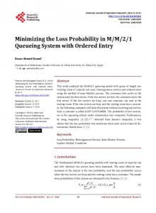
F i g u r e 1. rio v e r s u s a r r i v a l r a t e ~ for 01 = 3, 02 = 1 , / Z l = 20, # 2 = 10.
0.6
0.5
0.4
0.3
1-11 0.2
0.1
2
7 12 17 22 Figure 2. II 1 versus arrival rate A for 01 -- 3, 02 = 1, #1 -- 20, #2 -- 10.
27
of customers in the system, busy period of the s e r v e r / s y s t e m and waiting time of an arriving customer. In Figures 1-4, the values of the probabilities II0, rI1, 112, and YI3 are plotted against arrival rate ~ for chosen values of ~tl, ~t2, 01, and 02 satisfying the stability condition (2.1), p = A / ( # I + #2) < 1. By considering higher vacation rates (of order 104) in the vacation model under study, we o b t a i n a p p r o x i m a t e results for corresponding nonvacation models. For systems
M/M/2
Queueing System
1425
0.14
0.12
°°
.....
o..
0.1 '
"
with out vacation %
*
0.08 i"
o
Ia
H2 0.06
#r
Ir
•
v
~%1
I
0.04
0.02
2
7
12
k
17
22
27
22
27
Figure 3. H2 versus arrival rate A.
0.9 0.8
0.7 0.6 0.5
J
H3
0.4
o*Y with out vaca
0.3
•/
with vacation
0.2
0.1
o"
0 2
7
12
17
Figure 4. H3 versus arrival rate A,
with and with out vacation, the graphs of ri0 and I]3 indicate that the differences in probabilities steadily increase and decrease for increasing arrival rate A. Similar behaviour is displayed for the probabilities II1 and II2 also. From the Figure 5, it is seen that systems with larger values of vacation rates 01 and 02 can support larger values of A conforming to the stability condition. For higher values 01 and 02, i.e., for smaller mean vacation times for servers, the arrival rate of the system can be larger, since the servers are available on the average with the shorter break. We observe the same effect for
1426
B. KRISt[NA K1J1MARA N D S. PAVAI NIADHI~BWAR[
3° T 25
20 g~ = 15, 1~ = 20,/ 8~ =7,92=
~1 = 15, ~ = 2 0 ,
15
!a~ =20, ~ = 10,
E(N)
01 = 3, O= =~1,
~ = 20, ~ = 1O, 01=5, 62=7 0,=5, eo=7
."
10
:.-~-
-~'~-~ , ~.~.-=~.a.._-
~
12
7
~,
17
27
22
Figure 5. Mean system size E(N) versus arrival rate X.
30 p~ = 18, N = 18 with vacation
25 ii
with vacation J ,
20
~,=20,1-~=10 with out vacation
T A L,jf II
t i
15 /{
•
E(N} J
with vacation
I
" ~ . ...,.1" -"
!"
t
{
10
.--. 2
~ ~...-.-
• ~
,,-. ~
,, ~
=...a..
12 ~' 17 22 Figure 6. Mean system size E(N) versus axrival rate k. 7
with out vacation 27
different values of service rates #1 and #2. For increasing values of the service rates/~1 and #2, the customers are serw~d faster resulting in decrease of the mean number of customers in the system. The mean E(N) of the system size are plotted in Figure 6 against the arrival rate )~ for 01 = a and 02 = 1. It is observed t h a t the mean E?(N) of the system size steadily increases in unbounded fashion for system w i t h / w i t h o u t vacation. Further, the system with vacation has the mean system size growing much rapidly than the system without vacation.
M/M/2 Queueing System
1427
14
12
10
EqBS
4
2
7
12
;~
Figure 7. Mean busy period of the system versus arrival rate.
17
22
27
E(B) and mean server busy period E(BS)
14
/
12
/
10
! I
/
8 E(B 1~1=12' 1~=20 • vacation • wzth
::~_:--_----2_--'5---.
2
7
-
-
-
g1=20, ~ = 1 0 with vacation
1
/
/
/
'
.,,~/J/vac~Lon ...~,=!~,~=2o
.
.
]
^^ . ~ ' . ^
.
.
.
I
"'':-- : : ' ' - r
12
~,
Figure 8. Mean busy period of the system
17
22
E(B) versus arrival rate
27 A.
In F i g u r e 7, t h e v a c a t i o n model, it is seen t h a t t h e m e a n b u s y p e r i o d E(Bs) of t h e servers is less t h a n t h e m e a n b u s y p e r i o d E(B) of t h e s y s t e m . W h e n t h e a r r i v a l r a t e A increases t h e y b o t h converge to t h e s a m e value due to d e c r e a s i n g m e a n v a c a t i o n t i m e of t h e servers. F i g u r e 8 i n d i c a t e s t h a t t h e e x p e c t e d b u s y p e r i o d of t h e s y s t e m w i t h v a c a t i o n grows at a m u c h faster r a t e t h a n t h e s y s t e m w i t h o u t v a c a t i o n for values of traffic i n t e n s i t y p closer to one.
1428
B. KRISHNA KUMAR AND S. PAVAI MADHESWARI Table 1. M e a n s y s t e m size E(N) a n d m e a n w a i t i n g t i m e E(W) v e r s u s arrival r a t e A. Vacation Model for 01 = 3, 02 = 1 M e a n S y s t e m Size E(N)
M e a n W a i t i n g T i m e E(W)
A
ttl = 20, #2 = 10
#1 = 18, /~2 = 18
#1 = 12, #2 = 20
#1 = 20, /~2 = 10
#1 = 18, it2 = 18
#1 = 12, /~2 = 20
2
0.63286
0.619
0.6665
0.25339
0.2535
0.258
5
1.6184
1.5849
1.7548
0.25609
0.257
0.2724
10
3.4115
3.3631
4.0564
0.264
0.2678
0.3224
15
5.5651
5.5801
7.4803
0.2899
0.2996
0.417
20
8.555
8.6552
12.059
0.34853
0.3613
0.5257
25
13.9853
12.8748
18.1139
0.48539
0.44695
0.6529
28
24.598
16.2135
24.113
0.80869
0.5138
0.7934
N o n v a c a t i o n Model M e a n S y s t e m Size E(N)
M e a n W a i t i n g T i m e E(W)
A
#1 = 20, t~2 = 10
t~l = 18, #2 -----18
/xl = 12, #2 ----20
#1 = 20, #2 = 10
it1 = 18, ~2 = 18
#1 = 12, #2 = 20
2
O. 148465
O. 11156
O. 1329
0.00038639
0.000227
0.00032
5
0.3727
0.2835
0.3359
0.002133
0.001154
0.001702
10
0.79485
0.6027
0.7168
0.008897
0.004714
0.00706
15
1.3858
1.0095
1.2305
0.023156
0.011746
0.01808
20
2.4562
1.6087
2.0829
0.054629
0.02488
0.04073
25
5.51237
2.6846
4.0432
0.153148
0.051829
0.09874
28
14.5407
3.9398
7.5003
0.452396
0.08515
0.2051
Table 1 establishes the validity of Little's formula E(N) = A[E(W) + (1/2)(1/#1 + 1/#2)] with reasonable accuracy for the chosen parametric values for models with and without vacation.
6. C O N C L U S I O N For a two-server heterogeneous Markovian queueing system with the provision of multiple vacation, the matrix geometric technique has been used to study the stationary queue length distribution, busy period of the system, and waiting time distribution along with their means. Some numerical results have been obtained to display the effect of the system parameters on the performance measures.
REFERENCES 1. B.T. Doshi, Q u e u e i n g s y s t e m with v a c a t i o n s - - A survey, Queueing Systems 1, 29-66, (1986). 2. Y. Levy a n d U. Yechiali, Utilization of idle t i m e in an M / G / 1 q u e u e i n g s y s t e m , Management Science 22, 202-211, (1975). 3. J. T e g h e m , Control of t h e service process in a q u e u e i n g s y s t e m , European Journal of Operational Research 23, 141-158, (1986). 4. B.T. Doshi, Single-server q u e u e s with vacations, In Stochastic Analysis of Computer and Communications Systems, (Edited by H. Takagi), pp. 217-265, Elsevier, A m s t e r d a m , (1990). 5. H. Takagi, Queueing Analysis, A Foundation of Performance Evaluation, Volume 1: Vacation and Priority Systems, N o r t h - H o l l a n d , A m s t e r d a m , (1991). 6. Y. Levy a n d U. Yechiali, A n M / M / S q u e u e w i t h servers' vacations, Infor 14, 153-163, (1976). 7. E.P.C. K a o a n d K.S. Narayanan~ A n a l y s e s of an M / M / N q u e u e w i t h servers' vacations, European Journal of Operational Research 54, 256-266, (1991). 8. W . J . Gray, P.P. W a n g a n d M. Scott, Single c o u n t e r q u e u e i n g m o d e l s involving m u l t i p l e servers, Opsearch 3 4 (4), 283-296, (1997). 9. A. Tyagi, J. H a r m s a n d A. K a m a l , A n a l y s i s of M / M / S q u e u e s w i t h i - l i m i t e d service, Journal of Operational Research Society 53, 752-767, (2002). 10. I.L. M i t r a n y a n d B. A v i - I t z h a k , A m a n y server q u e u e with service i n t e r r u p t i o n s , Operations Research 16, 628-638, (1967).
M / M / 2 Queueing System
1429
11. M.F. Neuts and D.M. Lucantoni, A Markovian queue with N servers subject to breakdowns and repairs, Management Science 25, 849-861, (1979): 12. M.F. Neuts and Y. Takahashi, Asymptotic behaviour of the stationary distribution in the C I / P H / c queue with heterogeneous servers, Z. Wahrseheinlickeitsth 57, 441-452, (1981). 13. C. Latoche and V. Ramaswami, Introduction to Matrix Analytic Methods in Stochastic Modelling, ASASIAM, Philadelphia, PA, (1999). 14. M.F. Neuts, Matrix-Geometric Solutions in Stochastic Models: A n Algorithmic Approach, Johns Hopkins University Press, Baltimore, MD, (1981). 15. G. Latoche, A note on two matrices occurring in the solution of quasi-birth-and-death processes, Stochastic Models 3, 251-267, (1987). 16. J.G. Kemeny and J.L. Snell, Finite Markov Chains, Van Nostrand, Princeton, N J, (1960).