A Heuristic Search Approach to Solving the Software Clustering ...

A Heuristic Search Approach to Solving the Software Clustering Problem

A Thesis Submitted to the Faculty of Drexel University by Brian S. Mitchell in partial fufillment of the requirements for the degree of Doctor of Philosophy March 2002

c Copyright 2002

Brian S. Mitchell. All Rights Reserved.

ii

Acknowledgements Although a Ph.D. dissertation has a single name on the cover, it would be difficult to complete a Ph.D. program without a tremendous amount of support. There are many others who contributed to the success of this work. To these individuals I express my most sincere thanks. I would first like to recognize my advisor, S. Mancoridis. Dr. Mancoridis was a superior mentor, providing me with much needed encouragement, support, and guidance. I am also very proud to be the first member of Professor Mancoridis’ research group, which now has more than 10 active members inclusive of undergraduate, graduate, and doctoral students. I would also like to thank the other members of my committee: J. Johnson, C. Rorres, A. Shokoufandeh, and R. Chen for their input and thoughtful direction. Finally, I want to recognize a former member of my committee, Dr. L. Perkovic, for his contributions to my research. During my Ph.D. studies I also worked full-time as a software architect. Special thanks to my current and former supervisors who provided me with flexibility and guidance: J. O’Dell, B. Flock, L. Rowland, S. Fugale, L. Iovine, and R. Brooks. While I have many great colleagues, I specifically want to recognize: M. Killelea, S. Lupinacci, A. Chang, P. Cramer, J. Chauhan, A. Simone, C. Forrest, B. Cohen, D. Vista, B. Turner, R. Krupak, R. Halpin, S. Bergeron, J. Campisi, L. Stilwell, J. Weitzman, and B. Rodriguez for making work fun. Much of the work in this dissertation was funded with support from the National Science Foundation (NSF), AT&T Research Labs, and Sun Microsystems. Without financial backing, publishing and presenting this research would not have been possible. To my friends at the SERG Lab, I would like to thank you for your objective feedback on my ideas, and for rigorously critiquing my presentations prior to conferences.

iii I also want to recognize Pat Henry, the assistant department head, who provided much needed assistance with the courses that I taught at Drexel. My network of family and friends were also instrumental to enabling me to finish this project, while still remaining sane. They were always there to remind me that there are other things to do in life besides working on your computer. Finally, I want to acknowledge the person who sacrificed the most for me over the past 4 years – my wife Joann. Joann tolerated many days and nights with me working on my laptop, coming home late, and travelling. She was always supportive and there to provide much needed encouragement.

iv

Table of Contents List of Tables

. . . . . . . . . . . . . . . . . . . . . . . . . . . . . . . . . . viii

List of Figures . . . . . . . . . . . . . . . . . . . . . . . . . . . . . . . . . . Abstract

. . . . . . . . . . . . . . . . . . . . . . . . . . . . . . . . . . . . .

Chapter 1. Introduction . . . . . . . . . . . . . . . 1.1 Our Research . . . . . . . . . . . . . . . . . . 1.2 Understanding the Structure of Complex Software Systems . . . . . . . . . . . . . . . . 1.3 Overview of Our Software Clustering Process . 1.4 Distinguishing Characteristics of Our Software 1.5 Evaluating Software Clustering Results . . . . 1.6 Dissertation Outline . . . . . . . . . . . . . .

. . . . . . . . . . . . . . . . . . . . . . . . . . . . . . . . . . . . . . Clustering . . . . . . . . . . . .

Chapter 2. Background . . . . . . . . . . . . . . . . . . 2.1 Software Clustering Research . . . . . . . . . . . . 2.1.1 Bottom-Up Clustering Research . . . . . . . 2.1.2 Concept Analysis Clustering Research . . . 2.1.3 Data Mining Clustering Research . . . . . . 2.1.4 Top-Down Clustering Research . . . . . . . 2.1.5 Other Software Clustering Research . . . . . 2.1.6 Clustering Techniques used for Non-Software Engineering Problems . . . . . . . . . . . . 2.2 Clustering Techniques . . . . . . . . . . . . . . . . 2.2.1 Representation of Source Code Entities . . . 2.2.2 Similarity Measurements . . . . . . . . . . . 2.2.3 Clustering Algorithms . . . . . . . . . . . . 2.3 Observations . . . . . . . . . . . . . . . . . . . . . . 2.4 Source Code Analysis and Visualization . . . . . . . 2.4.1 Source Code Analysis . . . . . . . . . . . . . 2.4.2 Visualization . . . . . . . . . . . . . . . . . 2.5 Research Challenges Addressed in this Dissertation . . . . . . . . . . . . . . . . . . . . . .

ix xii 1 2

. . . . . . . . . . . . Approach . . . . . . . . . . . .

. . . . .

3 6 9 11 11

. . . . . . .

. . . . . . .

. . . . . . .

. . . . . . .

. . . . . . .

. . . . . . .

. . . . . . .

. . . . . . .

. . . . . . .

. . . . . . .

14 16 16 19 20 22 22

. . . . . . . . .

. . . . . . . . .

. . . . . . . . .

. . . . . . . . .

. . . . . . . . .

. . . . . . . . .

. . . . . . . . .

. . . . . . . . .

. . . . . . . . .

. . . . . . . . .

24 26 27 27 30 33 35 35 42

. . . . . . . . . .

48

v Chapter 3. Software Clustering Algorithms . . . . . . . . . 3.1 Representing the Structure of Software Systems . . . . . . 3.2 Evaluating MDG Partitions . . . . . . . . . . . . . . . . . 3.3 A Small Example . . . . . . . . . . . . . . . . . . . . . . . 3.4 Measuring Modularization Quality (MQ) . . . . . . . . . . 3.4.1 Basic MQ . . . . . . . . . . . . . . . . . . . . . . . 3.4.2 Turbo MQ . . . . . . . . . . . . . . . . . . . . . . . 3.4.3 Incremental Turbo MQ - ITurboMQ . . . . . . . . 3.4.4 Observations on the Complexity of Calculating MQ 3.5 Algorithms . . . . . . . . . . . . . . . . . . . . . . . . . . . 3.5.1 Exhaustive Search Algorithm . . . . . . . . . . . . 3.5.2 Hill-climbing Algorithm . . . . . . . . . . . . . . . 3.5.3 The Genetic Clustering Algorithm (GA) . . . . . . 3.6 Hierarchial Clustering . . . . . . . . . . . . . . . . . . . . 3.7 Chapter Summary . . . . . . . . . . . . . . . . . . . . . .

. . . . . . . . . . . . . . .

. . . . . . . . . . . . . . .

. . . . . . . . . . . . . . .

. . . . . . . . . . . . . . .

. . . . . . . . . . . . . . .

. . . . . . . . . . . . . . .

53 54 56 57 60 60 65 68 74 75 75 77 88 98 99

Chapter 4. The Bunch Software Clustering Tool . . . 4.1 Automatic Clustering using Bunch . . . . . . . . . . 4.1.1 Creating the MDG . . . . . . . . . . . . . . . 4.1.2 Clustering the MDG . . . . . . . . . . . . . . 4.2 Limitations of Automatic Clustering . . . . . . . . . 4.3 Bunch Enhancements . . . . . . . . . . . . . . . . . . 4.3.1 Omnipresent Module Detection & Assignment 4.3.2 Library Module Detection & Assignment . . . 4.3.3 User-Directed Clustering . . . . . . . . . . . . 4.3.4 Incremental Software Structure Maintenance . 4.3.5 Navigating the Subsystem Hierarchy . . . . . 4.4 Special User Features . . . . . . . . . . . . . . . . . . 4.5 Visualization and Processing of Clustering Results . . 4.6 Integration . . . . . . . . . . . . . . . . . . . . . . . . 4.7 User Directed Clustering Case Study . . . . . . . . . 4.8 Chapter Summary . . . . . . . . . . . . . . . . . . .

. . . . . . . . . . . . . . . .

. . . . . . . . . . . . . . . .

. . . . . . . . . . . . . . . .

. . . . . . . . . . . . . . . .

. . . . . . . . . . . . . . . .

. . . . . . . . . . . . . . . .

. . . . . . . . . . . . . . . .

. . . . . . . . . . . . . . . .

. . . . . . . . . . . . . . . .

101 102 102 105 110 113 113 115 116 117 119 121 124 125 125 132

Chapter 5. Distributed Clustering . . . . . . 5.1 Distributed Bunch . . . . . . . . . . . . . 5.1.1 Neighboring Partitions . . . . . . . 5.1.2 Distributed Clustering . . . . . . . 5.1.3 Adaptive Load-balancing . . . . . . 5.2 Distributed Clustering with Bunch . . . . 5.2.1 Setting up the BUI & BCS . . . . . 5.2.2 Setting up the Neighboring Servers 5.2.3 Clustering . . . . . . . . . . . . . . 5.3 Case Study . . . . . . . . . . . . . . . . . 5.3.1 Case Study Results . . . . . . . . . 5.4 Chapter Summary . . . . . . . . . . . . .

. . . . . . . . . . . .

. . . . . . . . . . . .

. . . . . . . . . . . .

. . . . . . . . . . . .

. . . . . . . . . . . .

. . . . . . . . . . . .

. . . . . . . . . . . .

. . . . . . . . . . . .

. . . . . . . . . . . .

133 134 135 136 141 143 143 145 147 147 149 151

. . . . . . . . . . . .

. . . . . . . . . . . .

. . . . . . . . . . . .

. . . . . . . . . . . .

. . . . . . . . . . . .

. . . . . . . . . . . .

vi Chapter 6. The Design of the Bunch Tool . . . . 6.1 A History of Bunch . . . . . . . . . . . . . . . . 6.2 Bunch Architecture . . . . . . . . . . . . . . . . 6.3 Design Patterns . . . . . . . . . . . . . . . . . . 6.4 Bunch Subsystems . . . . . . . . . . . . . . . . 6.4.1 The API Subsystem . . . . . . . . . . . 6.4.2 The Event Subsystem . . . . . . . . . . 6.4.3 The Bunch Graph & I/O Subsystems . . 6.4.4 The Cluster and Population Subsystem . 6.4.5 The Clustering Services Subsystem . . . 6.4.6 The Bunch Utilities Subsystem . . . . . 6.4.7 The Logging and Exception Management 6.5 Extending Bunch . . . . . . . . . . . . . . . . . 6.6 Using Bunch to Recover the Bunch Design . . . 6.7 Chapter Summary . . . . . . . . . . . . . . . .

. . . . . . . . . . . . . . . . . . . . . . . . . . . . . . . . . . . . . . . . . . . . . . . . . . . . . . . . . . . . . . . . . . . . . . . . . . . . . Subsystem . . . . . . . . . . . . . . . . . . . . .

Chapter 7. Similarity of MDG Partitions . . . . . . . . 7.1 Evaluating Software Clustering Results . . . . . . . . 7.2 Measuring Similarity . . . . . . . . . . . . . . . . . . 7.2.1 The MoJo Distance Similarity Measurement . 7.2.2 The Precision/Recall Similarity Measurement 7.2.3 Interpreting Similarity Results . . . . . . . . . 7.3 Our Similarity Measurements . . . . . . . . . . . . . 7.3.1 Edge Similarity Measurement - EdgeSim . . 7.3.2 Partition Distance Measurement - MeCl . . . 7.4 Isolating Certain Modules to Improve Similarity . . . 7.5 Comparative Study . . . . . . . . . . . . . . . . . . . 7.6 Chapter Summary . . . . . . . . . . . . . . . . . . .

. . . . . . . . . . . .

. . . . . . . . . . . .

Chapter 8. Evaluating MDG Partitions with the CRAFT 8.1 Establishing Confidence in Clustering Results . . . . . . 8.2 Our Framework - CRAFT . . . . . . . . . . . . . . . . . 8.2.1 A Small Example . . . . . . . . . . . . . . . . . . 8.2.2 The User Interface . . . . . . . . . . . . . . . . . 8.2.3 The Clustering Service . . . . . . . . . . . . . . . 8.2.4 The Data Analysis Service . . . . . . . . . . . . . 8.2.5 The Visualization Service . . . . . . . . . . . . . 8.3 Case Study . . . . . . . . . . . . . . . . . . . . . . . . . 8.4 Chapter Summary . . . . . . . . . . . . . . . . . . . . . Chapter 9. Conclusions and Future Research 9.1 Research Contributions . . . . . . . . . . . 9.2 Future Research Directions . . . . . . . . . 9.3 Closing Remarks . . . . . . . . . . . . . .

. . . . . . . . . . . . . . .

. . . . . . . . . . . . . . .

. . . . . . . . . . . . . . .

. . . . . . . . . . . . . . .

. . . . . . . . . . . . . . .

153 155 156 158 159 160 161 163 165 166 169 170 172 173 174

. . . . . . . . . . . .

. . . . . . . . . . . .

. . . . . . . . . . . .

. . . . . . . . . . . .

. . . . . . . . . . . .

175 176 177 178 180 181 182 182 185 189 191 195

Tool . . . . . . . . . . . . . . . . . . . . . . . . . . . . . . . . . . . .

. . . . . . . . . .

. . . . . . . . . .

. . . . . . . . . .

197 198 199 202 203 204 205 210 210 214

. . . .

. . . .

. . . .

216 217 218 222

. . . . . . . . . . . .

. . . . . . . . . . . .

Directions . . . . . . . . . . . . . . . . . . . . . . . . . . . . . . . .

. . . .

. . . .

vii Bibliography . . . . . . . . . . . . . . . . . . . . . . . . . . . . . . . . . . . 224 Appendix A. Programming Bunch . . . . . . . . . . . . . . . . . . . . A.1 Before You Begin Using Bunch . . . . . . . . . . . . . . . . . . . . A.2 Using the Bunch API . . . . . . . . . . . . . . . . . . . . . . . . . . A.3 An Example . . . . . . . . . . . . . . . . . . . . . . . . . . . . . . . A.4 Note to Old Users of the Bunch API . . . . . . . . . . . . . . . . . A.5 The Bunch API . . . . . . . . . . . . . . . . . . . . . . . . . . . . . A.5.1 Setting up the Clustering Activity . . . . . . . . . . . . . . . A.6 Understanding the Results of the Clustering Activity . . . . . . . . A.6.1 MQ Calculator Example . . . . . . . . . . . . . . . . . . . . A.7 Comprehensive Example . . . . . . . . . . . . . . . . . . . . . . . . A.8 Programmatically Processing the Results of the Clustering Activity A.8.1 Class BunchGraph . . . . . . . . . . . . . . . . . . . . . . . . A.8.2 Class BunchNode . . . . . . . . . . . . . . . . . . . . . . . . A.8.3 Class BunchEdge . . . . . . . . . . . . . . . . . . . . . . . . A.8.4 Class BunchCluster . . . . . . . . . . . . . . . . . . . . . . A.8.5 Example: Using the BunchGraph API . . . . . . . . . . . . .

. . . . . . . . . . . . . . . .

231 231 232 233 235 235 236 242 243 244 246 247 248 248 249 249

Appendix B. CRAFT User and Programmer B.1 Obtaining the CRAFT Tool . . . . . . . . B.2 Setup and Execution of the CRAFT Tool . B.3 Running CRAFT . . . . . . . . . . . . . . B.4 Developing a Custom Clustering Driver . . B.5 Special Considerations . . . . . . . . . . .

. . . . . .

256 256 256 257 258 261

Vita

Manual . . . . . . . . . . . . . . . . . . . . . . . . .

. . . . .

. . . . . .

. . . . . .

. . . . . .

. . . . . .

. . . . . .

. . . . . .

. . . . . .

. . . . . .

. . . . . . . . . . . . . . . . . . . . . . . . . . . . . . . . . . . . . . . . 262

viii

List of Tables 2.1

Dependencies of the Boxer System . . . . . . . . . . . . . . . . . . . . .

37

3.1 3.2 3.3 3.4

ITurboMQ Incremental Edge Type Updates . MDG Statistics for Some Sample Systems . . Explanation of the Hill-Climbing Algorithm . Clustering Statistics for Some Sample Systems

. . . .

. . . .

. . . .

. . . .

. . . .

. . . .

. . . .

. . . .

. . . .

. . . .

. . . .

. . . .

. . . .

. . . .

. . . .

73 74 80 86

5.1 5.2 5.3 5.4

Distributed Bunch Message Types . Testing Environment . . . . . . . . Application Descriptions . . . . . . Case Study Results . . . . . . . . .

. . . .

. . . .

. . . .

. . . .

. . . .

. . . .

. . . .

. . . .

. . . .

. . . .

. . . .

. . . .

. . . .

. . . .

. . . .

137 148 148 149

7.1 7.2

Similarity Comparison Results . . . . . . . . . . . . . . . . . . . . . . . . 191 Similarity Measurement Variance for linux . . . . . . . . . . . . . . . . 195

8.1 8.2

Similarity Results for CAT Test . . . . . . . . . . . . . . . . . . . . . . . 211 Performance of the CRAFT Tool . . . . . . . . . . . . . . . . . . . . . . 212

. . . .

. . . .

. . . .

. . . .

. . . .

. . . .

ix

List of Figures 1.1 1.2 1.3

The Bunch Software Clustering Environment . . . . . . . . . . . . . . . . The MDG for a Small Compiler . . . . . . . . . . . . . . . . . . . . . . . The Partitioned MDG for a Small Compiler . . . . . . . . . . . . . . . .

2.1 2.2 2.3 2.4 2.5 2.6 2.7 2.8

Classifying Software Features . . . . . . . . . . . . . . . . . . . . . The Relationship Between Source Code Analysis and Visualization The Structure of the Boxer System . . . . . . . . . . . . . . . . . . The Clustered Structure of the Boxer System . . . . . . . . . . . . The Structure of the rcs System . . . . . . . . . . . . . . . . . . . The Clustered Structure of the rcs System . . . . . . . . . . . . . . Inheritance Tree Showing Visual Conventions . . . . . . . . . . . . SHriMP View of Bunch . . . . . . . . . . . . . . . . . . . . . . . .

. . . . . . . .

. . . . . . . .

. . . . . . . .

29 35 38 38 40 41 46 47

3.1 3.2 3.3 3.4 3.5 3.6 3.7 3.8 3.9 3.10 3.11 3.12 3.13 3.14 3.15 3.16

Our Clustering Process . . . . . . . . . . . . . . . . . . . . . . . . . Module Dependency Graph of the File System . . . . . . . . . . . . Clustered View of the File System from Figure 3.2 . . . . . . . . . Intra-Connectivity Calculation Example . . . . . . . . . . . . . . . Inter-Connectivity Calculation Example . . . . . . . . . . . . . . . Modularization Quality Calculation Example . . . . . . . . . . . . . TurboMQ Calculation Example . . . . . . . . . . . . . . . . . . . . Two Similar Partitions of a MDG . . . . . . . . . . . . . . . . . . . Example move Operation for ITurboMQ . . . . . . . . . . . . . . . Neighboring Partitions . . . . . . . . . . . . . . . . . . . . . . . . . Example of a Building Block Partition . . . . . . . . . . . . . . . . Empirical Results for the Height of Partitioned MDG . . . . . . . . Example Crossover Operation . . . . . . . . . . . . . . . . . . . . . A Sample Partition . . . . . . . . . . . . . . . . . . . . . . . . . . . Structure of Mini-Tunis as Described in the Design Documentation Partition of Mini-Tunis as Derived Automatically using the GA . .

. . . . . . . . . . . . . . . .

. . . . . . . . . . . . . . . .

. . . . . . . . . . . . . . . .

57 58 59 61 62 63 67 69 71 78 84 87 90 92 95 96

4.1 4.2 4.3 4.4 4.5

The MDG File Format . . . . . . . . . . . . . . . . . . The MDG File for a Simple Compiler . . . . . . . . . . The MDG File for a Simple Compiler in GXL . . . . . Automatic Clustering with Bunch . . . . . . . . . . . . Automatically Partitioned MDG for a Small Compiler .

. . . . .

. . . . .

. . . . .

103 104 106 108 110

. . . . .

. . . . .

. . . . .

. . . . .

. . . . .

. . . . .

. . . . .

7 8 8

x 4.6 4.7 4.8 4.9 4.10 4.11 4.12 4.13 4.14 4.15

Omnipresent Module Calculator . . . . . . . . . . . . . . . . . . . . . . . Library Module Calculator . . . . . . . . . . . . . . . . . . . . . . . . . . User-directed Clustering Window . . . . . . . . . . . . . . . . . . . . . . Orphan Adoption Window . . . . . . . . . . . . . . . . . . . . . . . . . . Navigating the Clustering Results Hierarchy . . . . . . . . . . . . . . . . Bunch’s Main Window . . . . . . . . . . . . . . . . . . . . . . . . . . . . Bunch’s Miscellaneous Clustering Options . . . . . . . . . . . . . . . . . The Module Dependency Graph (MDG) of dot . . . . . . . . . . . . . . . The Automatically Produced MDG Partition of dot . . . . . . . . . . . . The dot Partition After Omnipresent Modules have been Identified and Isolated . . . . . . . . . . . . . . . . . . . . . . . . . . . . . . . . . . 4.16 The dot Partition After the User-Defined Clusters have been Specified . . 4.17 The dot Partition After the Adoption of the Orphan Module ismapgen.c . . . . . . . . . . . . . . . . . . . . . . . . . . . . . . . . .

114 115 117 118 120 122 123 126 126

5.1 5.2 5.3 5.4 5.5 5.6 5.7 5.8

Distributed Bunch Architecture . . . . . . . . . . . . Neighboring Partitions . . . . . . . . . . . . . . . . . Sample MDG and Partitioned MDG . . . . . . . . . Bunch Data Structures for Figure 5.3 . . . . . . . . . Distributed Bunch User Interface . . . . . . . . . . . Bunch Server User Interface . . . . . . . . . . . . . . Case Study Results for Small- and Intermediate-Sized Case Study Results for Large Systems . . . . . . . .

. . . . . . . .

. . . . . . . .

. . . . . . . .

. . . . . . . .

. . . . . . . .

. . . . . . . .

135 136 137 138 144 146 150 151

6.1 6.2 6.3 6.4 6.5 6.6 6.7 6.8 6.9 6.10 6.11

The Bunch Reverse Engineering Environment . . . . . . . . . . Bunch Architecture . . . . . . . . . . . . . . . . . . . . . . . . . The API Subsystem . . . . . . . . . . . . . . . . . . . . . . . . The Event Subsystem . . . . . . . . . . . . . . . . . . . . . . . The Bunch Graph & I/O Subsystems . . . . . . . . . . . . . . . The Cluster and Population Subsystem . . . . . . . . . . . . . . The Clustering Services Subsystem . . . . . . . . . . . . . . . . Collaboration Diagram for the Distributed Neighboring Process The Bunch Utilities Subsystem . . . . . . . . . . . . . . . . . . The Bunch Logging and Exception Management Subsystem . . The Structure of Bunch Factory Objects . . . . . . . . . . . . .

. . . . . . . . . . .

. . . . . . . . . . .

. . . . . . . . . . .

. . . . . . . . . . .

. . . . . . . . . . .

154 157 161 163 165 167 168 169 171 172 173

7.1 7.2 7.3 7.4 7.5 7.6 7.7

Example Dependency Graphs for a Software System . . . . . Two Slightly Different Decompositions of a Software System Another Example Decomposition . . . . . . . . . . . . . . . Example Clustering . . . . . . . . . . . . . . . . . . . . . . . The Υ Set from Figure 7.4 . . . . . . . . . . . . . . . . . . . The SubPartitions of A and B from Figure 7.4 . . . . . . . . Frequency Distribution for linux . . . . . . . . . . . . . . .

. . . . . . .

. . . . . . .

. . . . . . .

. . . . . . .

. . . . . . .

176 179 180 183 184 188 194

8.1 8.2

The User Interface of the CRAFT Tool . . . . . . . . . . . . . . . . . . . 200 The Architecture of the CRAFT Tool . . . . . . . . . . . . . . . . . . . . 201

. . . . . . . . . . . . . . . . . . . . . . . . . . . . . . Systems . . . . .

. . . . . . .

. . . . . . .

127 127 128

xi 8.3 8.4 8.5

A Small Example Illustrating the CRAFT Analysis Services . . . . . . . 202 Swing: Impact Analysis Results . . . . . . . . . . . . . . . . . . . . . . . 212 Confidence Analysis: A Partial View of Swing’s Decomposition . . . . . . 213

A.1 The Bunch API Environment . . . . . . . . . . . . . . . . . . . . . . . . 232 B.1 The User Interface of the CRAFT Tool . . . . . . . . . . . . . . . . . . . 257

xii

Abstract A Heuristic Search Approach to Solving the Software Clustering Problem Brian S. Mitchell Spiros Mancoridis

Most interesting software systems are large and complex, and as a consequence, understanding their structure is difficult. One of the reasons for this complexity is that source code contains many entities (e.g., classes, modules) that depend on each other in intricate ways (e.g., procedure calls, variable references). Additionally, once a software engineer understands a system’s structure, it is difficult to preserve this understanding, because the structure tends to change during maintenance. Research into the software clustering problem has proposed several approaches to deal with the above issue by defining techniques that partition the structure of a software system into subsystems (clusters). Subsystems are collections of source code resources that exhibit similar features, properties or behaviors. Because there are far fewer subsystems than modules, studying the subsystem structure is easier than trying to understand the system by analyzing the source code manually. Our research addresses several aspects of the software clustering problem. Specifically, we created several heuristic search algorithms that automatically cluster the source code into subsystems. We implemented our clustering algorithms in a tool named Bunch, and conducted extensive evaluation via case studies and experiments. Bunch also includes a variety of services to integrate user knowledge into the clustering process, and to help users navigate through complex system structures manually. Since the criteria used to decompose the structure of a software system into subsystems vary across different clustering algorithms, mechanisms that can compare different clustering results objectively are needed. To address this need we first examined two techniques that have been used to measure the similarity between system

xiii decompositions, and then created two new similarity measurements to overcome some of the problems that we discovered with the existing measurements. Similarity measurements enable the results of clustering algorithms to be compared to each other, and preferably to be compared to an agreed upon “benchmark” standard. Since benchmark standards are not documented for most systems, we created another tool, called CRAFT, that derives a “reference decomposition” automatically by exploiting similarities in the results produced by several different clustering algorithms.

1

Chapter 1 Introduction Software supports many of this country’s business, government, and social institutions. As the processes of these institutions change, so must the software that supports them. Changing software systems that support complex processes can be quite difficult, as these systems can be large (e.g., thousands or even millions of lines of code) and dynamic. Creating a good mental model of the structure of a complex system, and keeping that mental model consistent with changes that occur as the system evolves, is one of the many serious problems that confront modern software developers. This problem is exacerbated by other problems such as inconsistent or non-existent design documentation and a high rate of turnover among information technology professionals. Without automated assistance for gaining insight into the system design, a software maintainer often makes modifications to the source code without a thorough understanding of its organization. As the requirements of heavily-used software systems change over time, it is inevitable that adopting an ad hoc approach to software maintenance will have a negative effect on the quality of the system structure. Eventually, the system structure may deteriorate to the point where the source code organization is so chaotic that it needs to be overhauled or abandoned.

2 In an attempt to alleviate some of the problems mentioned above, the reverse engineering research community has developed techniques to decompose (partition) the structure of software systems into meaningful subsystems (clusters). Subsystems provide developers with high-level structural information about the numerous software components, their interfaces, and their interconnections. Subsystems generally consist of a collection of collaborating source code resources that implement a feature or provide a service to the rest of the system. Typical resources found in subsystems include modules, classes, and possibly other subsystems. Subsystems facilitate program understanding by treating sets of source code resources as high-level software abstractions. The large amount of research effort directed at the software clustering problem is a good indication that there is value in creating abstract structural views of large programs. However, each of the clustering techniques described in the literature uses a different criterion to determine clusters. Thus, it is not accurate to state that these clustering approaches recover the structure of a software system. Instead these clustering techniques produce structural views of source code based on assumptions about good system design characteristics. Hence, for software clustering to be useful, researchers and practitioners must (a) investigate the tradeoffs associated with using different clustering algorithms for different types of systems, and (b) evaluate individual clustering results against accepted benchmark standards.

1.1

Our Research

Software clustering algorithms and tools are useful for simplifying program maintenance, and improving program understanding. Our research addresses these objectives by defining algorithms and creating tools that are designed to be used, integrated and extended by other researchers. We describe our clustering algorithms in Chap-

3 ters 3, 5, and 7, and address the design of our tools in Chapters 6 and 8. Furthermore, in Chapter 9 we argue for the importance of using software clustering technology with different representations of a system’s structure in order to understand and document its overall architecture. We also noticed that most researchers use the opinion of system designers to determine the effectiveness of clustering techniques, and the quality of their produced results. While this evaluation approach is appropriate for commonly studied systems, for which an agreed upon structural decomposition exits, it offers little value to software practitioners who want to use software clustering technology on other systems. To improve this evaluation practice, we implemented several measurements to establish the degree of “similarity” between system decompositions in a formal way. We also created a tool that produces a benchmark decomposition of a software system automatically, based on common trends found in the results of different clustering algorithms. This work advances the state of practice in software clustering research by providing alternative ways to evaluate software clustering results.

1.2

Understanding the Structure of Complex Software Systems

Software Engineering textbooks [74] advocate the use of documentation as an essential tool for describing a system’s intended behavior, and for capturing the system’s design structure. In order to be useful to future software maintainers, a system’s documentation must be current with respect to any software changes. In practice, however, we often find that accurate design documentation does not exist. While documentation tools such as javadoc [35] make the task of searching for key documentation in source code easier, these tools are of little value to software practitioners who are trying to understand the more subtle abstract aspects of a system’s design.

4 In the absence of informal advice from system designers, or up-to-date documentation about a system’s structure, software maintainers are left with few choices. They can inspect the source code manually to develop a mental model of the system organization. Unfortunately, this approach is often not practical because of the large number of relations between the source code components. Another alternative is to use automated tools to produce information about the system structure. A primary goal of these tools is to analyze the entities and relations in the source code, and to cluster them into meaningful subsystems. Subsystems facilitate program understanding by collecting the detailed source code resources into higher-level abstract entities. Subsystems can also be organized hierarchically, allowing developers to study the organization of a system at various levels of detail by navigating through the hierarchy. Unfortunately, subsystems are not specified in the source code explicitly, and the subsystem structure is not obvious from the source code structure. Although many programming languages have evolved to support the specification of higher-level system concepts such as objects and components, these languages still do not support the explicit definition of subsystems. We have, however, seen some developments in programming language design that enables programmers to group source code entities into structures that can be used to represent higher-level system behavior. While these language features support organizing source code into subsystems, the actual assignment of source code entities into commonly named structures relies on programmer convention. For example, consider Java packages and C++ namespaces. These programming language features associate different source code entities (e.g., classes) with a common name. When we discuss the architecture of our clustering tool in Chapter 6, we describe how we used the package naming feature of Java to organize the source code of our clustering tool in accordance to its subsystem structure.

5 As most programming languages lack the descriptiveness necessary to specify subsystems, researchers have investigated other ways to document abstract software system structures. One example is Module Interconnection Languages (MIL) [14, 64, 9, 46], which support the specification of software designs that include subsystem structures. Mancoridis [46] presents another approach to specifying system components (including subsystems) and dependencies that is based on the Interconnection Style Formalism (ISF). ISF is a visual formalism for specifying structural relationships, and constraints on these relationships. One problem with MILs and ISF is that they produce documentation that must be maintained independently of the source code. A well-known problem in software engineering is keeping external documentation consistent with the source code as the system undergoes maintenance. Even without programming language support for subsystems, the original developers of a system often organize source code into subsystems by applying software development best-practices. This informal organization is often based on directory structure, or file naming conventions. For example, consider the FileSystem subsystem of an operating system. We would expect this subsystem to include modules that support local files, remote files, mounting file systems, and so on. The question is, in the absence of this knowledge from designers, can the key subsystems of a software system be mined directly from the source code? We think that the answer to this question is yes. Thus far, however, creating tools to do so has proven to be difficult because clustering software systems into subsystems automatically is a hard problem. To illustrate this point consider representing the structure of a software system as a directed graph.1 The graph is formed by representing the modules of the system as nodes, and the relations between the modules

1

Most research on the software clustering problem represents the structure of a software system as a directed graph.

6 as edges. Each partition of the software structure graph is defined as a set of nonoverlapping clusters that cover all of the nodes of the graph. The goal is to partition the graph in such a way so that the clusters represent meaningful subsystems. Clustering systems using only the source code components and relationships is a hard problem, as the number of all possible ways to partition a software structure graph grows exponentially with respect to the number of its nodes [50]. The general problem of graph partitioning (of which software clustering is a special case) is NPhard [22]. Therefore, most researchers have addressed the software clustering problem by using heuristics to reduce the execution complexity to a polynomial upper bound.

1.3

Overview of Our Software Clustering Process

Figure 1.1 illustrates the software clustering process that is supported by a tool that we created called Bunch. The upper left side of this figure shows a collection of source code files as the input to our process, and the upper right side shows the visualized clustering results as the output of our process. The first step in the clustering process is to extract the module-level dependencies from the source code and store the resultant information in a database. Readily available source code analysis tools that support a variety of different programming languages can be used for this step. After all of the module-level dependencies have been stored in a database, a script is executed to query the database, filter the query results, and produce, as output, a textual representation of the module dependency graph (MDG). We define MDGs formally in Section 3.1, but for now, consider the MDG as a graph that represents the modules (classes) in the system as nodes, and the relations between modules as weighted directed edges. Once the MDG is created, Bunch applies our clustering algorithms to the MDG and creates a partitioned MDG. The clusters in the partitioned MDG represent subsystems, where each subsystem contains one or more modules from the source code.

7 Bunch Clustering Tool

Source Code void main() { printf(“Hello World!”); }

Visualization Tools dotty

Tom Saywer

User Interface

Source Code Analysis Tools Clustering Algorithms Acacia

Chava

cia

Partitioned MDG Tools

MDG File M1

M1

M3

M3 M6

M6 M2 M7 M4

M8

Programming API

M5

M2 M7 M4

M8

M5

Figure 1.1: The Bunch Software Clustering Environment

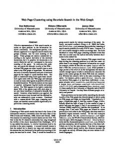
The goal of Bunch’s clustering algorithms is to determine a partition of the MDG that represents meaningful subsystems. After the partitioned MDG is created, we use graph drawing tools such as dotty [62] or Tom Sawyer [77] to visualize the results. An example MDG for a small compiler developed at the University of Toronto is illustrated in Figure 1.2. We show a sample partition of this MDG, as created by Bunch, in Figure 1.3. Notice how Bunch created four subsystems to represent the abstract structure of a compiler. Specifically, there are subsystems for code generation, scope management, type checking, and parsing. The center of Figure 1.1 depicts additional services that are supported by the Bunch clustering tool. These services are discussed thoroughly in subsequent chapters of this dissertation.

8

main

parser

codeGenerator

typeChecker

argCntStack

scopeController

dictIdxStack

typeStack

addrStack

dictionary

dictStack

scanner

declarations

Figure 1.2: The MDG for a Small Compiler

(SS-L0):parser

(SS-L0):codeGenerator

parser (SS-L0):scopeController scopeController

dictionary

dictIdxStack

dictStack

main (SS-L0):typeChecker

scanner

typeChecker

typeStack

codeGenerator

argCntStack

addrStack

declarations

Figure 1.3: The Partitioned MDG for a Small Compiler

9

1.4

Distinguishing Characteristics of Our Software Clustering Approach

Many of the software clustering algorithms presented in the literature use different criteria and techniques to decompose the structure of software systems into clusters. Given a particular system, the results produced by the clustering algorithms differ because of the diversity in the approaches employed by the algorithms. As will be described in Chapter 2, much of the clustering research has focused on introducing new clustering techniques, or validating the results of existing ones. Our focus is on creating search-based algorithms and tools to cluster large software well and in an efficient manner. Hence, we have developed the Bunch tool that includes a fully-automatic clustering engine, and is complemented by additional features to integrate designer knowledge into the automated clustering process. Bunch also includes a programmer’s API so that our clustering tool can be integrated with other tools, and a flexible design that enables Bunch to be extended by others. Bunch offers several distinguishing capabilities as compared to other clustering tools that have been developed by the reverse engineering research community. Specifically: • Most software clustering tools can be categorized as either fully-automatic, semiautomatic, or manual. Fully-automatic tools decompose a system’s structure without any manual intervention. Semi-automatic tools require manual intervention to guide the clustering process. Manual software clustering techniques guide the user through the clustering process. Bunch includes a fully-automated clustering engine, and implements several clustering algorithms. Additionally, a user may supply any known information about a system’s structure to Bunch. This information is respected by the automatic clustering engine. Bunch also includes several tools to help users obtain information about the system’s components, and their interrelations. In

10 other words, our clustering approach provides fully-automatic, semi-automatic, and manual clustering features.

• Most software clustering algorithms are deterministic, and as such, always produce the same result for a given input. Since our approach is based on randomized heuristic search techniques, our clustering algorithms often do not produce the same result, but a family of similar results. We address the beneficial aspects of this behavior in Chapter 8.

• Most software clustering algorithms are computationally intensive. This limits their ability to cluster large systems within a reasonable amount of time. While we have improved the performance of our clustering approach dramatically over the past couple of years,2 our clustering algorithms may be paused at any time in order to generate a valid solution. In general, the quality of the solution improves the longer Bunch runs.3

• The Internet has enabled us to simplify the distribution of our clustering tools to researchers, students and software engineers. The Bunch tool has been available on the Drexel University Software Engineering Research Group (SERG) [70] web site for unrestricted non-commercial use since 1998. Since Bunch was developed using the Java programming language, users can execute Bunch on the Windows, Solaris, Linux, and any other operating system that supports a Java Virtual Machine (JVM). Furthermore, as is discussed in Chapter 6, our clustering tools were designed to be extended and integrated with other tools.

2

The current release of Bunch is able to cluster a system the size of Linux, with approximately 1,000 modules and 10,000 relations, in a few minutes. 3 This type of algorithm is typically referred to as an any time algorithm [86, 87].

11

1.5

Evaluating Software Clustering Results

Many of the clustering techniques published in the literature present case studies, where the results are evaluated by consulting the designers and developers of the system being studied. This evaluation technique is very subjective. Recently, researchers have begun developing infrastructure to evaluate clustering techniques, in a semi-formal way, by proposing similarity measurements [2, 3, 52]. These measurements enable the results of clustering algorithms to be compared to each other, and preferably to be compared to an agreed upon “benchmark” standard. Note that the “benchmark” standard needn’t be the optimal solution in a theoretical sense. Rather, it is a solution that is perceived by several people to be “good enough”. Evaluating software clustering results against a benchmark standard is useful and often, in the process, exposes interesting and surprising design flaws in the software being studied. However, this kind of evaluation is not always possible, because benchmark standards are often not documented, and the developers are not always accessible for consultation. We have thus developed a tool, called CRAFT, which shows how the results produced by Bunch and other clustering tools can be evaluated in the absence of a reference design document or without the active participation of the original designers of the system. CRAFT essentially creates a “reference decomposition” by exploiting similarities in the results produced by several clustering algorithms. The underlying assumption is that, if several clustering algorithms agree on certain clusters, these clusters become part of the generated reference decomposition.

1.6

Dissertation Outline

In this chapter we introduced the software clustering problem, and outlined our approach to addressing this problem. The remainder of this section provides an overview of the chapters in this dissertation.

12 • Chapter 2 - Background This chapter is a survey of software clustering approaches. It examines clustering techniques that have been applied in computer science, mathematics, science, and engineering, and investigates how these techniques have been adapted to work in the software domain. The chapter concludes with a discussion of research challenges related to software clustering, providing motivation and perspective for our research.

• Chapter 3 - Software Clustering Algorithms This chapter describes three search-based clustering algorithms that we have developed. These algorithms accept a graph representation of a software system’s structure as input, and automatically produce a partitioned (clustered) graph as output. Both formal and empirical complexity analyses of our algorithms are provided in this chapter.

• Chapter 4 - The Bunch Clustering Tool This chapter presents how the algorithms described in Chapter 3 are implemented in the Bunch tool. The features of Bunch are described, along with a case study that demonstrates the effectiveness of using Bunch for software maintenance and program understanding.

• Chapter 5 - Distributed Clustering This chapter covers an enhancement made to the Bunch implementation to support distributed clustering. The distributed clustering algorithm is presented, along with a case study that demonstrates the effectiveness of using distributed techniques to cluster very large systems.

13 • Chapter 6 - The Design of the Bunch Tool Chapter 6 describes the design of the Bunch tool. Interesting design features of Bunch are presented. Specifically, we comment on how we overcame common problems related to implementing research systems. Emphasis is placed on Bunch’s design aspects that support extension and integration. • Chapter 7 - Similarity of MDG Partitions Being able to compare clustering results is a requirement for evaluating the effectiveness of clustering algorithms. This chapter describes two similarity measurements that have been used to compare clustering results, and highlights some significant problems with them. Next, two new similarity measurements that we designed and implemented are presented. This chapter concludes with a case study that demonstrates the effectiveness of our similarity measurements. • Chapter 8 - Evaluating MDG Partitions with the CRAFT Tool It is important that users of software clustering tools have confidence that the results produced by this technology are good. Ideally, a documented benchmark decomposition is available for comparison, although in reality such benchmarks rarely exist. In this chapter we suggest some ways to create a benchmark standard, and present a tool, named CRAFT, that determines a benchmark decomposition by analyzing a collection of different software clustering algorithm results. • Chapter 9 - Conclusions The final chapter in this dissertation summarizes the contributions of our work to the field of software clustering, and suggests future research opportunities.

14

Chapter 2 Background Over the past few years there has been significant research activity in the field of reverse engineering. There are several reasons for this. First, immediately prior to the year 2000, information technology professionals spent significant amounts of time verifying that their software will work into the new century. Much of this software was remediated to work after the year 2000 by programmers who had no access to the designers of the system that they were changing. Second, there have been rapid changes in the software development processes. Just in the past few years we have seen information technology systems migrate from two-tiered, to three-tiered, to n-tiered1 (browser-based) client/server architectural models. We have also seen development approaches change from structured, to object-oriented, to componentoriented. Each time the system architecture changes, developers must understand how

1 Industry literature commonly refers to n-tiered architectures as systems that are decomposed into presentation (user-interface), application logic, and data access components. Each tier exposes an interface that may be deployed on a different computer and accessed over a computer network. Two-tiered architectures separate the data access from the presentation and application logic, which are combined into a single tier. Three-tiered architectures are designed with logical independence between the presentation, application logic, and data access components. With n-tiered architectures, the application logic and data access components are typically distributed across many physical hardware systems, and the presentation layer is often constructed using browser technology. Middleware frameworks such as Microsoft’s DCOM, Javasoft’s EJB, and CORBA typically are used to facilitate the distribution between the application components.

15 to adopt the previous version of their software to fit a new architectural model. The above situations are forcing software professionals to understand, and in some cases, remodularize vast amounts of source code. Software clustering tools can help these individuals by providing automated assistance for recovering the abstract structure of large and complex systems. In the earliest days of computing, the need for clustering low-level software entities, into more abstract structures (called modules) was identified. The landmark work of David Parnas [63] first suggested that the “secrets” of a program should be hidden behind module interfaces. The resultant information hiding principle advocated that modules should be designed so that design decisions are hidden from all other modules. Parnas suggested that interfaces to modules should be created to supply a well-defined mechanism for interacting with the modules’ internal algorithms. Parnas advocated a programmer discipline whereby procedures that act on common data structures should be grouped (clustered) into common modules. Much of the basis for objectoriented design techniques evolved from Parnas’s ideas. Objected-oriented techniques provide an initial level of clustering by grouping related data, and functions that operate on the data, into classes. Booch [5] suggests that during the design process a system should be decomposed into collaborating autonomous agents (a.k.a. objects) to perform higher-level system behavior. Booch stresses the importance of using abstraction in design to focus on the similarities between related objects, encapsulation to promote information hiding, organizing design abstractions into hierarchies to simplify understanding, and using modularity to promote strong cohesion and loose coupling between classes.2 Almost all research in software clustering concentrates on one or more of these concepts.

2

Cohesion and coupling measure the degree of component independence. Cohesion is a measurement of the internal strength of a module or subsystem. Coupling measures the degree of dependence between distinct modules or subsystems. According to Sommerville [74], well designed systems should exhibit high cohesion and low coupling.

16 Given the importance of helping software professionals understand the structure of source code, the remainder of this chapter will review work performed by researchers in the area of software clustering.

2.1

Software Clustering Research

This section examines research that has been performed in the area of software clustering. These works are classified into bottom-up, top-down, data mining, and concept analysis clustering techniques. The end of this section describes miscellaneous approaches that have been applied by researchers to the software clustering problem.

2.1.1

Bottom-Up Clustering Research

In an early paper on software clustering, Hutchens and Basili [30] introduce the concept of a data binding. A data binding classifies the similarity of two procedures based on the common variables in the static scope of the procedures. Data bindings are very useful for modularizing software systems because they cluster procedures and variables into modules (e.g., helpful for migrating a program from COBOL to C++). The authors of this paper discuss several interesting aspects of software clustering. First, they identify the importance of keeping a system’s reverse engineered model consistent with the designer’s mental model of the system’s structure. The authors also claim that software systems are best viewed as a hierarchy of modules, and as such, they focus on clustering methods that exhibit their results in this fashion. Finally, the paper addresses the software maintenance problem, and identifies the benefit of using clustering technologies to verify how the structure of a software system changes or deteriorates over time. Robert Schwanke’s tool Arch [68], provides a semi-automatic approach to software clustering. Arch is designed to help software engineers understand the current system

17 structure, reorganize the system structure, integrate advice from the system architects, document the system structure, and monitor compliance with the recovered structure. Schwanke’s clustering heuristics are based on the principle of maximizing the cohesion of procedures placed in the same module, while at the same time, minimizing the coupling between procedures that reside in different modules. Arch also supports an innovative feature called maverick analysis. With maverick analysis, modules are refined by locating misplaced procedures. These procedures are then prioritized and relocated to more appropriate modules. Schwanke also investigated the use of neural networks and classifier systems to modularize software systems [69]. In Hausi M¨ uller’s work, one sees the basic building block of a cluster change from a module to a more abstract software structure called a subsystem. Also, M¨ uller’s tool, Rigi [57], implements many heuristics that guide software engineers during the clustering process. Many of the heuristics discussed by M¨ uller focus on measuring the “strength” of the interfaces between subsystems. A unique aspect of M¨ uller’s work is the concept of an omnipresent module. Often, when examining the structure of a system, modules that act like libraries or drivers are found. These modules provide services to many of the other subsystems (libraries), or consume the services of many of the other subsystems (drivers). M¨ uller defines these modules as omnipresent and contends that they should not be considered when performing cluster analysis because they obscure the system’s structure. One last interesting aspect of M¨ uller’s work is the notion that the module names themselves can be used as a clustering criteria. Later in this section we mention a paper by Anquetil and Lethbridge [3], which investigates this technique in more detail. The work of Schwanke and M¨ uller resulted in semi-automatic clustering tools where user input and feedback is required to obtain meaningful results. Choi and Scacchi’s [9] paper describes a fully-automatic clustering technique that is based on maximizing the cohesion of subsystems. Their clustering algorithm starts with a di-

18 rected graph called a resource flow diagram (RFD) and uses the articulation points of the RFD as the basis for forming a hierarchy of subsystems. The RFD is constructed by placing an arc from A to B if module A provides one or more resources to module B. Their clustering algorithm searches for articulation points, which are nodes in the RFD that divide the RFD graph into two or more connected components. Each articulation point and connected component of the RFD is used as the starting point of forming subsystems. Choi and Scacchi also used the NuMIL [60] architectural description language to specify the resultant design of the system. They argue that NuMIL provides a hierarchical description of modules and subsystems, which cannot be specified directly in the flat structure of the system’s source code. Mancoridis, Mitchell et al. [50, 49, 16, 54] treat the software clustering problem as a search problem. One key aspect of our clustering technique is that we do not attempt to cluster the native source code entities directly into subsystems. Instead, we start by generating a random subsystem decomposition of the software entities. We then use heuristic searching techniques to move software entities between the randomly generated clusters, and in some cases we even create new clusters, to produce an “improved” subsystem decomposition. This process is repeated until no further improvement is possible. The search process is guided by an objective function that rewards high cohesion and low coupling. We have used several heuristic search techniques that are based on hill-climbing and genetic algorithms. The original version of our tool clustered source code into subsystems automatically. In fact, it is the fully automatic clustering capability of Bunch that distinguishes it from related tools that require user intervention to guide the clustering process. However, we have extended Bunch over the past few years to incorporate other useful features that have been described, and in some cases implemented, by other researchers. For example, we incorporated Orphan Adoption techniques [82] for incremental structure maintenance, Omnipresent Module support [57], and user-

19 directed clustering to complement Bunch’s automatic clustering engine. The clustering algorithms, tools, and evaluation frameworks supported by Bunch are the primary subject of this dissertation.

2.1.2

Concept Analysis Clustering Research

Lindig and Snelting [45] developed a software modularization technique that uses mathematical concept analysis [73]. In their paper, they present a technique for modularizing source code structures along with formal definitions for an abstract data object (module), cohesion, coupling, and a mathematical concept. Their work is conceptually similar to Hutchens and Basili [30], where the goal is to cluster procedures and variables into modules based on shared global variable dependencies between procedures. The first step in their software modularization technique is to generate a variable usage table. This table captures the shared global variables that are used by each procedure in the system. The authors then present a technique for converting the table into a concept lattice. A concept lattice is a convenient way to visualize the variable relationships between the procedures in the system. The next step in their modularization technique involves systematically updating procedure interfaces to remove dependencies on global data (i.e., the variable can be passed via the procedures interface instead). The goal is to transform the concept lattice into a tree-like structure. Once this transformation is accomplished, the modules are formed from the concept lattice. The authors describe two techniques for accomplishing this transformation: modularization by interface resolution and modularization via block relations. Unfortunately, due to performance problems, the authors were not able to modularize two large systems as part of their case study. Furthermore, their technique would probably only be useful for analyzing systems that are developed using programming languages that rely on global data for information sharing (i.e., COBOL, FORTRAN). Thus, their technique would not be well-suited for object-oriented programming languages, where data is typically encapsulated behind class interfaces.

20 van Deursen and Kuipers [15] examined the use of cluster and concept analysis to identify objects from COBOL code automatically. Their approach to object identification consists of the following steps: (1) classify the COBOL records as objects, (2) classify the procedures or programs as methods, and (3) determine the best object for each method using clustering techniques. The authors start by creating a usage matrix that cross references the relations between modules and variables (from COBOL records). Once this matrix is formed, they use a hierarchial agglomerative clustering algorithm [39] that is similar to Arch [68]. Clusters are formed using a dissimilarity measurement based on calculating the Euclidian distance between the variables in the usage matrix. The authors also investigated the use of concept analysis to determine clusters from the variables in the usage table. For this approach, the usage table is transformed into a concept table by considering the items (variable names) and features (usage of variable(s) in modules). Once the items and features are determined, the authors determine the concepts by locating the maximal collection of items that share common features. As with Lindig and Snelting’s approach, the concepts can be represented as a lattice. Since the concept lattice shows all possible groupings of common features, the clusters can be determined at various levels of detail by moving from the bottom to the top of the lattice.

2.1.3

Data Mining Clustering Research

Montes de Oca and Carver [12] present a formal visual representation model for deriving and presenting subsystem structures. Their work uses data mining techniques to form subsystems. We agree with the author’s claim that data mining techniques are complementary to the software clustering problem. Specifically:

• Data mining has been used to find non-trivial relationships between elements in a database. Software clustering tries to solve a similar problem by forming

21 subsystem relationships based on non-obvious relationships between the source code entities. • Data mining can discover interesting relationships in databases without upfront knowledge of the objects being studied. One of the significant benefits of software clustering is that it can be used to promote program understanding. As mentioned in Section 1.2, developers who work with source code are often unfamiliar with the intended structure of the system. • Data mining techniques are designed to operate on a large amount of information. Thus, the study of data mining techniques may advance the state of current software clustering tools. Clustering tools typically suffer from performance problems due to the large amount of data that needs to be processed to develop the subsystem structures. The authors use the dependencies of procedures on shared files as basis for forming subsystems. However, they do not describe in detail how their similarity mechanism works, as the primary goal of their research was to develop a formal visualization model for describing subsystems, modules, and relationships. We believe, however, that the authors were able to articulate a good set of requirements for visualizing software clustering results. For example, their visualization approach supports hierarchical nesting, and singular programs, which are programs that do not belong to a subsystem. Singular programs are very similar in concept to M¨ uller’s omnipresent modules [57]. Application of data mining approaches to the software clustering problem was also investigated by Sartipi et al. [67, 66]. The authors clustering approach involved using data mining techniques to annotate nodes in a graph representing the structure of a software system with association strength values. These association strength values are then used to partition the graph into clusters (subsystems).

22

2.1.4

Top-Down Clustering Research

Most approaches to clustering software systems are bottom-up. These techniques produce high-level structural views of a software system by starting with the system’s source code. Murphy’s work with Software Reflexion Models [59] takes a different approach by working top-down. The goal of the Software Reflexion Model is to identify differences that exist between a designer’s understanding of the system structure and the actual organization of the source code. By understanding these differences, a designer can update his model, or the source code can be modified to adhere to the organization of the system that is understood by the designer. This technique is particularly useful to prevent the system’s structure from “drifting” away from the intended system structure as a system undergoes maintenance. Eisenbarth, Koschke and Simon [17] developed a technique for mapping a system’s externally visible behavior to relevant parts of the source code using concept analysis. Their approach uses static and dynamic analyses to help users understand a system’s implementation without upfront knowledge about its source code. Data is collected by profiling a system feature while the program is executing. This data is then processed using concept analysis to determine a minimal set of feature-specific modules from the complete set of modules that participated in the execution of the feature. Static analysis is then performed against the results of the concept analysis to identify further feature-specific modules. The goal is to reduce the set of modules that participated in the execution of the feature to a small set of the most relevant modules in order to simplify program understanding. The authors conducted a case study using two open source web browsers. They were able to examine various features of these web browsers and map them to a small percentage of source code modules.

2.1.5

Other Software Clustering Research

In a paper by Anquetil, Fourrier and Lethbridge [2], the authors conducted experiments on several hierarchal clustering algorithms. The goal of their research is to

23 measure the impact of altering various clustering parameters when applying clustering algorithms to software remodularization problems. The authors define three quality measurements that allow the results of their experiments to be compared. Of particular interest is the expert decomposition quality measurement. This measurement quantifies the difference between two clustering results, one of which is usually the decomposition produced by an expert. The measurement has two parts: precision (agreement between the clustering method and the expert) and recall (agreement between the expert and the clustering method). The authors claim that many clustering methods have good precision and poor recall. Anquetil et al. also claim that clustering methods do not “discover” the system structure, but instead, impose one. Furthermore, they state that it is important to choose a clustering method that is most suited to a particular system. We feel that this assessment is correct, however, imposing a structure that is consistent with the information hiding principle is often desired, especially when the goal is to gain an understanding of a system’s structure in order to support software maintenance. As such, we find that many similarity measures are based on maximizing cohesion and minimizing coupling. Anquetil et al. make another strong claim, namely that clustering based on naming conventions often produce better results than clustering using information extracted from source code structure. Clustering algorithms that are based on naming conventions group entities with similar source code file names and procedure names. Anquetil and Lethbridge [3] presented several case studies that show promising results (high precision and high recall) using name similarity as the criterion to cluster software systems. For some systems, using name-base software clustering produces good results because, by convention, programmers organize their source files into different directories, and name source code files that perform a related function in a similar way. How-

24 ever, for some systems, this approach may not work well, especially when a system has undergone maintenance by programmers that did not understand the system’s structure thoroughly. Using source code features as the basis for clustering always provides accurate information to a clustering method, as this information is extracted directly from the code. Tzerpos’ and Holt’s ACDC clustering algorithm [80] uses patterns that have been shown to have good program comprehension properties to determine the system decomposition. The authors define 7 subsystem patterns and then describe their clustering algorithm that systematically applies these patterns to the software structure. After applying the subsystem patterns of the ACDC clustering algorithm, most, but not all, of the modules are placed into subsystems. ACDC then uses orphan adoption [82] to assign the remaining modules to appropriate subsystems. Koschke’s Ph.D. thesis [42] examines 23 different clustering techniques and classifies them into connection-, metric-, graph-, and concept-based categories. Of the 23 clustering techniques examined, 16 are fully-automatic and 7 are semi-automatic. Koschke also created a semi-automatic clustering framework based on modified versions of the fully-automatic techniques discussed in his thesis. The goal of Kochke’s framework is to enable a collaborative session between his clustering framework and the user. The clustering algorithm does the processing, and the user validates the results.

2.1.6

Clustering Techniques used for Non-Software Engineering Problems

Numerous clustering approaches have been investigated by the graph theory research community to solve problems related to pattern recognition, VLSI wire routing, data mining, web-based searching, and so on. Like software clustering, these algorithms try to identify groups of related items in an input set; however, the “groups”

25 are not subsystems, and the “input set” is not generated from the relations in the source code. When clustering approaches are being used for non-software engineering problems several aspects must be considered to ensure that the quality of the clustering results are good. As an example, Fasulo’s [18] paper examines four clustering algorithms and analyzes their strengths and weaknesses. The author’s goal is to help users decide which type of clustering algorithm works best for each type of application. Fasulo classifies the most important features of a clustering technique. These features must be considered prior to applying a clustering technique to a particular problem: 3 • Data and Cluster Model: The representation of the input data and anticipated cluster structure produced by a clustering algorithm. • Scalability: The ability of the algorithm to cluster the input data within a reasonable amount of time and computing capacity. • Noise: The ability to identify and isolate nodes in the input set that do not naturally cluster with other nodes. • Parameters: Understanding the clustering algorithm parameters, and how they impact the clustering results. • Result Presentation: How the clustering results are presented to the user. Since most graph partitioning techniques are computationally expensive, researchers have also investigated ways to improve the performance of clustering algorithms without sacrificing quality too much. One such example is discussed in a paper by Karypis and Kumar [38] where the authors investigate multilevel graph partitioning schemes. Multilevel partitioning techniques first reduce the size of the input graph by collapsing vertices and edges. This new, smaller graph is then partitioned, followed by an

3

We address each of these features for our software clustering approach in Chapters 3 & 4.

26 uncoarsening process to construct a partition for the original graph. Other graph partitioning techniques that use spectral methods [37] are discussed by Karypis and Kumar. Because spectral clustering algorithms are computationally expensive, multilevel techniques are often used to improve performance, at the cost of somewhat worse partition quality. Karypis and Kumar’s paper subsequently investigates several options for refining the multilevel partitioning process with the goal of producing good clustering results at a reasonable cost. A case study is presented to show the results of applying their multilevel clustering algorithms to 33 different types of graphs that are commonly encountered in mathematics, science and engineering. The clustering approaches examined by the graph theory community tend to represent the input to the clustering process as an undirected graph. This representation has some desirable properties such as being able to model the input graph as a symmetric matrix. Our techniques for clustering software systems use directed graphs that are created from relations in the source code. These graphs are asymmetric because the input to our clustering algorithms (i.e., the MDG) models the resources consumed by the modules in the system. For example, if Module A calls a function in Module B, we draw an arc in the MDG from A to B to indicate that A uses a resource provided by B.

2.2

Clustering Techniques

In this section we examine techniques that use source code as the input into the clustering process. Using the source code as input to a clustering algorithm is a good idea since source code is often the most up-to-date software documentation. As a starting point, the survey paper by Wiggerts [83] describes three fundamental issues that need to be addressed when designing clustering systems: 1. Representation of the entities to be clustered. 2. Criteria for measuring the similarity between the entities being clustered. 3. Clustering algorithms that use the similarity measurement.

27

2.2.1

Representation of Source Code Entities

When clustering source code components, several things must be considered to determine how to represent the entities and relations in the software system. There are many choices depending on the desired granularity of the recovered system design. First, should the entitles be procedures and methods, or modules and classes? Next, the type of relations between the entities needs to be established. Should the relationships be weighted, to provide significance to special types of dependencies between the entities? For example, are two entities more related if they use a common global variable? How should this weight compare to a pair of entities that have a dependency that is based on one entity using the public interface of another entity? As an example, in the Rigi tool, the user sets the criteria used to calculate the weight of the dependency between two entities. In Chapter 3 we describe our approach to representing software structures. Furthermore, in Section 9.2, we suggest that identifying system entities and determining the weight of the relations between entities, warrants additional study.

2.2.2

Similarity Measurements

Once the type of entities and relations for a software system are determined, the “similarity” criteria between pairs of entities must be established. Similarity measures are designed so that larger values generally indicate a stronger similarity between the entities. For example, the Rigi tool establishes a “weight” to represent the collective “strength” of the relationships between two entities. The Arch tool uses a different similarity measurement where a similarity weight is calculated by considering common features that exist, or do not exist, between a pair of two entities. Wiggerts classifies the approach used by the abovementioned tools as association coefficients. Additional similarity measurements that have been classified are distance measures, which deter-

28 mine the degree of dissimilarity between two entities, correlation coefficients, which use the notion of statistical correlation to establish the degree of similarity between two entities, and probabilistic measures, which assign significance to rare features that are shared between entities (i.e., entities that share rare features may be considered more similar than entities that share common features).

Example Similarity Measurements 1. Arch: The Arch similarity measurement [69] is formed by normalizing an expression based on features that are shared between two software entities, and features that are distinct to each of the entities: Sim(A, B) =

W (a ∩ b) 1 + c × W (a ∩ b) + d × (W (a − b) + W (b − a))

In Arch’s similarity measurement, c and d are user-defined constants that can add or subtract significance to source code features. W (a ∩ b) represents the weight assigned to features that are common to entity A and entity B. W (a−b) and W (b−a) represent the weights assigned to features that are distinct to entity A and entity B, respectively. 2. Rigi: Rigi’s primary similarity measurement, Interconnection Strength (IS), represents the exact number of syntactic objects that are exchanged or shared between two components. The IS measurement is based on information that is contained within a system’s resource flow graph (RFG). The RFG is a directed graph G = (V, E), where V is the set of nameable system components, and E ⊆ V × V is a set of pairs hu, vi which indicates that component u provides a set of syntatic objects to component v. Each edge hu, vi in the RFG contains an edge weight (EW) that is labeled with the actual set of syntactic objects that component u provides to component v. For example, if class v calls a method in

29 class u named getCurrentTime(), then getCurrentTime() would be included in the EW set that labels the edge from u to v in the RFG. Given the RFG, and the EW set for each edge in the RFG, the IS similarity measurement is calculated as follows: P rv(s) =

S

xV

EW (s, x)

Req(s) =

S

xV

EW (x, s)

ER(s, x) = Req(s) ∪ P rv(x) EP (s, x) = P rv(s) ∪ Req(x)

IS(u, v) = |ER(u, v)| + |EP (u, v)| Thus, the interconnection strength IS between a pair of source code entities is calculated by considering the number of shared exact requisitions (ER) and exact provisions (EP) between two modules. ER is the set of syntactic objects that are needed by a module and are provided by another module. EP is the set of syntactic objects that are provided by a module and needed by another module. Both ER and EP are determined by examining the set of objects that are provided by a module, Prv(s), and the set of objects that are needed (requisitioned) by a module Req(s). 3. Other classical similarity measurements: Wiggerts presents a few similarity measurements in his software clustering survey [83]. These measurements are based on classifying how a particular software feature is shared, or not shared between two software entities. Consider the table shown in Figure 2.1.

Entity i

Entity j 1 0 1

a

b

0

c

d

a: b: c: d:

Number of common features in Entity i and Entity j Number of features unique to Entity i Number of features unique to Entity j Number of features absent in both Entity i and Entity j

Figure 2.1: Classifying Software Features

30 Given the table in Figure 2.1, similarity measurements can be formed by considering the relative importance of how features are shared between two software entities. An interesting example is d, which represents the number of 0-0 matches, or the number of features that are absent in both entities. According to Wiggerts, the most commonly used similarity measurements are:

simple(i, j) =

a+d a and Jaccard(i, j) = a+b+c+d a+b+c

Thus, the simple measurement treats 0-0 (type d) and 1-1 (type a) matches equally. The Jaccard measurement does not consider 0-0 matches. In a recent paper, Anquetil et al. [2] applied the simple and Jaccard similarity measurements to cluster Linux, Mosaic, gcc, and a large proprietary legacy telecommunication system. Using their decomposition quality measurement, the authors determined that the Jaccard tends to gives better results than the simple measurement.

2.2.3

Clustering Algorithms

Now that representation and similarity measures have been discussed, we direct our attention to describing some common algorithms used for software clustering. Although many algorithms have been used for clustering, most of them arrange their clusters hierarchically. Hierarchical clustering algorithms generally start with the low-level source code entities (i.e., modules and classes). These entities are then clustered into subsystems, which in turn, are clustered into larger subsystems (i.e., subsystems that contain other subsystems). Eventually, everything coalesces into a single cluster, resulting in a tree of clusters, where the leafs of the tree are the source code entities, and the interior nodes of the tree are the subsystems.

31 Hierarchies are found in many domains because they allow problems to be studied at different levels of detail by navigating up and down the levels of the hierarchy. This property is particularly useful when clustering techniques are used to understand the structure of complex systems because of the large amount of data that must be considered. Below, we present an example showing the clustering algorithms used by several existing clustering tools: • One of the simplest clustering algorithms is implemented by the Rigi tool. In Rigi, two software entities are merged into a common subsystem if the similarity measure (i.e., Interconnection Strength) between them exceeds the value of a user-defined threshold. • Arch uses the hierarchical agglomerative clustering approach shown in Algorithm 1. Algorithm 1: Classical Hierarchial Clustering Algorithm Place each entity in a subsystem by itself repeat 1: Identify the two most similar entities 2: Combine them into a common subsystem until the results are “satisfactory”; van Deursen and Kuipers [15] use a similiar algorithm to cluster COBOL code into objects. The main difference between their approach and Arch is that a different similarity measurement is used to group the entities into clusters. Additionally, van Deursen and Kuipers continue the merge process until everything coalesces into a single cluster, forming a dendrogram. They then suggested how to establish a cut point in the dendrogram to determine the clusters. • The clustering algorithm described Anquetil and Lethbridge [3] is based on using the names of the source code files to form subsystems. In their paper the authors

32 present several techniques for decomposing file names into abbreviations. The high-level algorithm for this clustering approach is shown in Algorithm 2. Algorithm 2: Using Source Code Files to Create Subsystems 1: Split each file name into a set of abbreviations formed by substrings in the file names (e.g., FileSystem = {“file”,“sys”,“system”}). 2: Create an abbreviation dictionary from all of the substrings derived from the file names. 3: For each abbreviation in the dictionary, create a concept, and label it with its abbreviation. 4: For each file name, put it into each of the concepts that correspond to its abbreviations (derived in Step 1). 5: Use heuristics to determine the clusters from the concepts. Anquetil et al. proposed several heuristics for creating clusters from the concepts that are defined in Step 5 of Algorithm 2. The authors favor the “first abbreviation” heuristic, which involves placing the selected file into a cluster based on the first abbreviation of the file name that is not a single letter. The authors observed that the first abbreviation of a file name (i.e., the abbreviation with the highest precedence) is a good candidate for determining the cluster to which it belongs, while subsequent abbreviations tend to represent additional concepts. For example, a module named FileSystem, containing the abbreviations {“file”,“sys”,“system”} would be placed into the “file” cluster.

33

2.3

Observations

In the previous sections of this chapter we surveyed software clustering research and presented several well-known clustering techniques. In examining this work, several interesting observations can be made:

• Much of the clustering research mentions coupling and cohesion. Low coupling and high cohesion [74] are generally recognized properties of well-designed software systems. However, there does not seem to be a consistent and formal definition for these properties. • Many clustering algorithms are computationally intensive. In Section 1.2, we show that clustering software systems by partitioning a graph is a NP-hard [22] problem. Many researchers address this complexity by creating heuristics, which reduce the computation complexity so that results can be obtained in a reasonable (i.e., polynomial) amount of time. • Software clustering researchers often use experts to validate the results of their techniques. While such subjective evaluation provides insight into the quality of a clustering result, formal methods for validating the results of a clustering technique are needed. Recent work by Antquetil and Lethbridge [3, 2] begin to address this problem. Specifically, they define measurements for precision and recall, which quantify the differences between an expert’s view and a clustered view of a systems structure. This is perhaps better than an expert’s “opinion” about how good or bad a clustered result is. A recent paper by Tzerpos and Holt [79] takes this concept one step further. In their paper, they define a distance metric called MoJo that can be used to evaluate the similarity of two decompositions of a software system. Thus, using MoJo, the distance between an expert’s decomposition and a clustering tool’s decomposition of a software

34 system can be measured. In Chapter 7 we examine these measurements further, and propose two new similarity measurements called MeCl and EdgeSim. Our similarity measurements overcome some problems that we discovered with precision/recall and MoJo when we used them to evaluate our own clustering algorithms. • Many researchers recognize that a fundamental software engineering problem is that the structure of systems deteriorates as they undergo maintenance. To address this problem Tzerpos and Holt [82] present an orphan adoption technique to update an existing system decomposition incrementally by investigating how a change to the system impacts its existing structure. One problem with orphan adoption, however, is that it only examines the impact of the changed (or new) module(s) on the existing system structure. Without considering the remaining (existing) system components and relationships, the structure of the system can decay over time by applying the orphan adoption technique repeatedly unless a complete remodularization is performed periodically. Tzerpos and Holt’s [79] work on MoJo can also help explain the impact of maintenance on a software system. By applying MoJo to two versions of a software system, a measurement for the differences between their structures can be obtained. Thus, if MoJo produces a large result, one should expect that there are significant structural differences between the two versions of the system. • Early clustering research focused on clustering procedures into modules and classes. As software systems continued to grow, the research focus switched to clustering modules and classes into higher-level abstractions such as subsystems. In the next section of this chapter we introduce source code analysis and software visualization, which are two important bodies of work that are related to software clustering.

35

2.4

Source Code Analysis and Visualization

Clustering tools typically rely on source code analysis and visualization tools as shown in Figure 2.2. Source Code Analysis

Representation Similarity Measurements Clustering Algorithms

Visualization

Figure 2.2: The Relationship Between Source Code Analysis and Visualization In order to improve usability, clustering tools should enable a user to provide source code as input to the clustering process. Because typical systems of interest are large and complex, it is desirable to avoid having to transform the source code into the representation (e.g., MDG) required by the clustering tool manually. Not only is this manual task tedious and highly error prone, but researchers often want to cluster the same software system iteratively by varying the parameters supported by the clustering tool without having to revisit the original source code. Another complementary technology to software clustering is visualization. The output of the clustering process often contains a large amount of data that needs to be presented to users. Without effective visualization techniques, it is difficult to present the results of the clustering process in a useful way.

2.4.1

Source Code Analysis

Source code analysis has been researched for many years because it is useful to consolidate a system’s source code into a single repository that can be used for a variety of program understanding and reverse engineering activities. Repositories are use-

36 ful to developers because they allow them to investigate the program structure by navigating through the many intricate relations that exist between the source code components. In addition to clustering, source code analysis tools have been applied to other activities such as performing dead code detection, program slicing, and reachability analysis. The first step in source code analysis is to parse the source code and store the parsed artifacts in a repository. Source code analysis tools often support a variety or programming languages such as COBOL, C, C++, Java and Smalltalk. Once the repository is populated with data obtained from the source code, queries can be made against the repository to extract structural information about the source code. Two popular approaches to organizing the internal structure of the repository include storing the system’s abstract syntax tree, or structuring the repository as a relational database. The AT&T Research Labs have created a family of source code analysis tools that support C, C++, and Java. Their approach is based on an entity relationship model [7]. For each supported language, the source code is scanned and a relational database is constructed to store the entities (e.g., file names, variables, functions, macros), and relations (e.g., variable reference, function call, inheritance in a program). In addition to the entities and relations, various attributes are recorded about the entities and relations such as data types, usage, an so on. Once the relational database is constructed, a series of tools are available to query the database and produce information about the structure of the system being studied. The output of the query operation can be saved as a delimited text file. The query tools provided by AT&T can then be combined with other standard Unix tools, such as AWK, to further process the data. Table 2.1 illustrates the result of running an AWK script that queries and filters the repository for the Boxer graph drawing system. Each row in the table consists

37

Table 2.1: Dependencies of the Boxer System Module 1 main main main main main main main main main boxParserClass boxParserClass boxParserClass boxParserClass boxParserClass boxParserClass boxParserClass boxParserClass boxClass boxClass boxClass boxClass boxClass Globals hashedBoxes GenerateProlog GenerateProlog stackOfAny boxScannerClass stackOfAnyWithTop

Module 2 boxParserClass boxClass edgeClass Fonts Globals Event hashedBoxes GenerateProlog colorTable Globals error boxScannerClass boxClass edgeClass stackOfAnyWithTop colorTable hashedBoxes edgeClass Fonts colorTable MathLib hashedBoxes boxClass hashGlobals boxClass Globals nodeOfAny Lexer stackOfAny

38 main

Event

GenerateProlog

Fonts

boxParserClass

Globals

boxScannerClass

boxClass

Lexer

hashedBoxes

MathLib

error

stackOfAnyWithTop

stackOfAny

edgeClass

colorTable

nodeOfAny

hashGlobals

Figure 2.3: The Structure of the Boxer System of a pair that represents a relation between two modules in the Boxer system. For example, the tuple (main, boxParserClass) indicates that a relation exists between the main module and the boxParserClass module. Table 2.1 only shows the dependencies between pairs of modules. Using the query tools provided by AT&T, one could capture additional information such as the relation type (e.g., global variable reference), a weighted average for the relative “strength” of the dependency, and so on. 11 main 6

15 boxParserClass

Event

GenerateProlog

1 stackOfAnyWithTop

error

boxScannerClass

0

Globals 16

stackOfAny

Lexer

boxClass

7 nodeOfAny

hashedBoxes

MathLib

edgeClass

colorTable

Fonts

hashGlobals

Figure 2.4: The Clustered Structure of the Boxer System The data presented in Table 2.1 is visualized in Figure 2.3 to show the structure of the Boxer drawing tool. Because this is a small system, consisting of 18 modules and

39 relatively few dependencies, the overall structure of Boxer should be comprehensible by inspecting the figure. Sometimes, however, even small systems can be difficult to understand. Figure 2.5 shows the graph of the relations recovered by performing source code analysis on rcs, an open source version control tool. Clearly, because of the number of relations, it is impractical to develop a mental model for the structure of rcs by simply inspecting the graph. When our clustering tool, Bunch, was applied to the relationships for the Boxer and rcs systems, the graphs illustrated in Figure 2.4 and Figure 2.6 were produced. Figures 2.4 and 2.6 present a clustered view of the Boxer and rcs systems, which show the source code components clustered into subsystems. The clustered view of the source code often highlights information that is not obvious in the unclustered view of the same software system. Source code analysis tools traditionally require access to the source code of the system in order to build a repository. Java’s platform independent bytecode, enables code analysis to be performed on the compiled bytecode, eliminating the need for the actual source code. Several software engineering tools have been constructed that require only Java bytecode. Womble [33], extracts a system’s object model directly from its Java bytecode. Rayside, Kerr and Kontogannis [65] constructed a tool to detect changes between different versions of Java systems using bytecode. Chava [41] complements the suite of source code analysis tools developed by AT&T for languages such as C [7] and C++ [8]. Chava works with both the Java source code and the compiled bytecode. As indicated earlier, clustering tools require source code analysis tools to package the source code into a representation where the relations between the source code entities can be analyzed. Another important requirement for a clustering tool is the ability to present the results of the clustering process to the user in a meaningful way.

40

rcs.c

ci.c

co.c

rcsclean.c

rcsgen.c

rcsdiff.c

rcsfcmp.c

rcsmerge.c

rcsedit.c

rcstime.c

merge.c

merger.c

maketime.c

rcslex.c

partime.c

rcsfnms.c

partime.h

rcssyn.c

rcsrev.c

rcsutil.c

ident.c

rcskeep.c

rlog.c

maketime.h

rcsmap.c

rcskeys.c

version.c

rcsbase.h

conf.h

Figure 2.5: The Structure of the rcs System

41

(SS-L0):rcsedit.c co.c

(SS-L0):rcssyn.c rcsdiff.c

rcsmerge.c

rcsclean.c

(SS-L0):merger.c rcs.c

merge.c

(SS-L0):rcsfnms.c rcsgen.c

ci.c

(SS-L0):rcslex.c rcsrev.c

rlog.c

(SS-L0):rcsfcmp.c merger.c

rcsedit.c

rcskeep.c

rcsfcmp.c

(SS-L0):partime.h maketime.c

rcstime.c

rcssyn.c

rcslex.c

(SS-L0):conf.h

(SS-L0):ident.c

partime.c

maketime.h

ident.c

partime.h

conf.h

version.c

rcsfnms.c

(SS-L0):rcsbase.h rcsutil.c

rcsmap.c

rcsbase.h

Figure 2.6: The Clustered Structure of the rcs System

rcskeys.c

42 In the next section we discuss the importance of visualization tools. In particular, we discuss tools that are used extensively by researchers for graph visualization. We also present some open problems associated with using graph drawing tools for the purpose of presenting software clustering results.

2.4.2

Visualization

The goal of a graph visualization tool is to present a graph clearly. Unfortunately, because most systems of interest are large and complex, providing a visualization of large structures that is easy to interpret by a user is difficult. There are several reasons for this difficulty: Navigation • Most visualization tools only provide simple navigation and zooming facilities. This limitation often makes it difficult to see the clustered result at a sufficient level of detail. • When presenting clustering results to the user, it is desirable to first present a high-level view of the system structure, and then allow the user to drill-down into more detailed views that show the internal structure of a selected high-level component. Most visualization tools do not support this capability.

Interpretation • Most visualization tools present results using traditional directed, or undirected graphs. While graphs show the relationships between source code entities, clustering results have additional dimensions that need to be included in the visualization. For example, it is desirable to show the entities that are clustered into common subsystems along with the relative strength of the relationships between the entities. To address some of these problems, some visualization

43 tools support the labeling of nodes and edges. Although these features are helpful when viewing small graphs, they add additional clutter to large and highly-interconnected graphs. • Some clustering tools produce multiple views of a system’s structure. For example, one view may illustrate the clustered subsystems, another view may describe the inheritance hierarchy, and so on. It would be desirable to have a visualization tool that organizes and integrates these different views of the system.

Integration • Many visualization tools are tightly integrated into CASE environments, which makes their integration with other tools difficult.

The above list details a few common problems with visualization tools. Not all tools exhibit all of the problems described above, but none are capable of addressing all of the described issues. The remainder of this section reviews some visualization tools that have been used by clustering systems. Figures 2.3, 2.4, 2.5, and 2.6 were created using the AT&T graph layout tool named dot [62]. Dot is a versatile graph drawing tool that has been used by researchers for many years. One notable feature of dot is its graph description language. Users specify the nodes and edges of the graph in a text file, and may add any number of optional attributes to the nodes and edges in order to control the appearance of the graph. For example, users can set attributes to control the font, font size, edge style, edge labels, colors of the nodes and edges, fill types, scaling, and so on. The dot documentation [62] contains a complete description of the plethora of options that can be included in a dot input file.

44 Dot is a command line utility that accepts a dot description file as input, and produces output in any one of 12 different supported output file formats (e.g., GIF, JPEG, PostScript, etc.). The dot layout engine uses advanced techniques to increase the clarity of the produced graph by performing operations such as edge routing and edge crossing minimization. While dot produces an output file, a complementary research tool by AT&T, called dotty [62], is an online graph viewer. Dotty can be used to visualize and edit a graph that is specified in a dot description file. Dotty supports many common visualization functions such as birdseye views and zooming. The simplicity of the dot description language, along with the power of the dot engine, allows dot and dotty to be integrated with other tools easily. Tom Sawyer [77] is a commercial graph visualization tool that we have integrated with our clustering tools. Tom Sawyer supports a text file description language that is not as robust as the dotty graph description file. However, Tom Sawyer supports many different layouts that make it easier to view the relationships between source code entities and subsystems. Both dotty and Tom Sawyer allow users to specify the size, location, color, style, and label of the objects in the graph. These features are particularly useful when visualizing clustered systems because these attributes can be used to represent additional program understanding aspects. For example, the size of the nodes in the graph can be altered so that larger modules are “bigger” than smaller modules. Also, the thickness, style, grayscale or color of the edges in the graph can be adjusted to represent the “strength” of the relationship between two modules in the graph. In a recent paper by Demeyer, Ducasse, and Lanza [13], the authors describe many visualization conventions based on node size, node position, node color, and edge color that represent different aspects of the structure of a software system. These techniques allow many dimensions of a software system’s structure to be visualized

45 at the same time (in 2D), however, the user must continuously keep in mind what each visual convention means. Figure 2.7 illustrates an example showing some of the conventions described by Demeyer et al. In this figure, a small inheritance tree is shown. The nodes represent the classes, and the edges represent the inheritance relationships. The width of each node represents the number of instance variables in a class, and the height of each node represents the number of methods in the class. Finally, the color tone of the nodes represent the number of class variables. Once the different conventions of the figure are understood, the two dimensional graph presents much useful information to the user. The conventions specified above are implemented in a tool called CodeCrawler [13]. It is unclear how difficult it would be to integrate CodeCrawler into another utility because the authors do not describe an application programming interface, or a file format. Another graphical modelling approach designed to represent structural design information is presented by Montes de Oca and Carver [12]. The authors present a visual model called the Representation Model (RM), which consists of simple graphical objects and connectors. Each object represents a structural aspect of the system (e.g., program, module, file, subsystem), and each connector represents a dependency within the system (e.g., a program uses a file). RM uses a hierarchical visualization approach where the initial diagram presented to the user represents the high-level view of the system. Each high-level RM object is linked to another RM diagram that visualizes additional detail about the internals of the initial RM object. This layering continues, forming a hierarchy of RM diagrams, until a primitive level is reached. The authors of the paper describe the model and plan to create an automated tool for creating, viewing and managing RM documents. Currently, RM documents are created manually in an external CASE or diagramming tool.

46

Figure 2.7: Inheritance Tree Showing Visual Conventions

47

Figure 2.8: SHriMP View of Bunch

48 The SHriMP [75](Simple Hierarchical Multi-Perspective) technique is designed to visualize hierarchial data, and as such, it can help users to navigate and understand complex software structures. The SHriMP tool presents a nested graph view of the software structure, where the detailed nodes can represent the source code, and the higher-level nodes can represent subsystems.4 Navigation within the SHriMP environment is based on a hypertext link-following metaphor. SHriMP combines the hypertext metaphor with animated panning and zooming over the nested graph in order to help the user navigate the visualization. The SHriMP tool can be downloaded from the Internet [72]. Figure 2.8 illustrates a SHriMP view of Bunch’s source code. The top of this figure illustrates the high-level visualization of Bunch. Each of the small boxes represents a class, and each of the lines represents a relationship. The relationships are colored to distinguish between their types (e.g., inheritance, method invocation, etc.). One of the boxes in the topmost figure is a little larger than the others. This box represents the GenericClusteringMethod class from Bunch’s source code. Drilling down into this module results in the view shown in the middle of Figure 2.8. At the bottom of Figure 2.8, another view is rendered on the GenericClusteringMethod class by performing an additional “zoom” operation. At this level of detail, the source code for the class is presented.

2.5

Research Challenges Addressed in this Dissertation

This chapter presents a survey of software clustering research. Specifically, it describes clustering techniques that create module-level and subsystem-level system decompositions as well as tools that have been used for software clustering.

4

SHriMP was designed to visualize many aspects of software systems, examining a subsystem decomposition is just one example.

49 Based on the current state of practice of software clustering research discussed in this chapter, we made several observations that we have used to guide our research. These research objectives are described in subsequent chapters of this dissertation:

• Improving Performance. In order to cluster a software system, a large amount of data must be analyzed. Since many clustering tools are computationally intensive, they do not perform well when applied to large systems. To address this problem, we have integrated distributed techniques to scale our clustering approach [54] (see Chapter 5). For environments where highperformance computers are not available, the distributed computation approach used by the SETI project [71] should also be investigated for its applicability to the software clustering problem. Data Mining techniques, as described by Montes de Oca and Carver [12] and Sartipi et al. [67, 66], may also help address performance challenges associated with software clustering algorithms.

• Dynamic Analysis. Many of the systems being developed today do not have all of their dependencies specified in the source code. Instead, these systems use Application Programming Interfaces (API’s) provided by the operating system or programming language to load their classes (or modules) dynamically at runtime. Once loaded, the functionality provided by these components is invoked indirectly via a reference or proxy to the dynamically loaded component. Thus, to gain a good understanding of the structure of these systems, the runtime dependencies must be captured and included in the model of the system structure to be clustered. Technology provided by runtime debuggers and the Java Virtual Machine may provide a starting point for capturing these dynamic dependencies. To address the need for dynamic analysis, the clustering infrastructure presented in this dissertation has been used to create the Gadget

50 and Form tools [70]. These tools were developed in support of two M.Sc. theses at Drexel University [47, 51].

• Representing Software Structures. In Section 2.2.1 we discuss the importance of representing the entities and relations of a software system. Many software clustering algorithms and similarity measurements rely on the weight of the relations to make clustering decisions. The type of relations in software systems may be function calls, variable references, macro invocations, and so on. An open problem is to establish the collective weight of the relations that exist between the modules and classes in the system. Typically, all relations are treated equally, however, biasing the relations – so that certain types of dependencies are more significant than others – may be a good idea for improving clustering algorithms. Since most clustering techniques use graphs to represent software systems, it would also be interesting to investigate the similarities and difference between software structure graphs and other types of graphs such as random, bipartite, connected, and directed acyclic graphs. We describe the representation used by our clustering techniques in Chapters 1 and 3, and methods to compare software structure graphs in Chapter 7. Additionally, in Chapter 9, we argue that future work on representing the structure of software systems is needed.

• Improving Clustering Techniques. In Chapter 3 we describe three search algorithms that we have created to solve the software clustering problem. Our algorithms use heuristic search techniques to create clusters, and have been described in our papers [50, 16, 49, 54]. Early versions of our clustering algorithms required improvement in order to cluster large systems efficiently. In Chapter 3 we not only discuss our basic clustering algorithms, but we also describe some

51 of the improvements that we have made over the years to be able to handle large systems. Our focus has been on improving the efficiency of our hill-climbing algorithms by creating objective functions that are computationally cheaper to evaluate, and integrating features such as Simulated Annealing [40]. In Chapter 3 we also describe our Genetic Algorithm (GA) for clustering [16]. GA’s have been shown to produce good results in optimizing large problems. Although our initial results with GA’s are promising, we feel that additional study is needed. We are especially interested in alternative encoding schemes, as the performance and results of applying GA’s to optimization problems is highly dependent on the encoding of the problem. Some suggestions for improving our GA approach is described in Section 3.5.3. • Incremental Clustering. As a system undergoes maintenance, there is a risk that the structure of the system will drift from its intended design. One would expect that minor changes to the source code would not alter the system structure drastically. Thus, if an investment has already been made in decomposing a system into subsystems, it would be desirable to preserve this information as a starting point for updating, and in some cases, creating new subsystems. The Orphan Adoption [82] technique is a first step in addressing this problem. Due to the large computational requirements necessary to re-cluster a system each time it changes, we feel that the topic of incremental clustering warrants additional study. Chapter 4 describes how Orphan Adoption was implemented in our clustering techniques. • Comparative Evaluation. Most of the case studies reported in the clustering research literature are conducted on small and medium sized systems. There are enough clustering techniques to warrant investigation of how these algorithms

52 perform against a set of systems of different sizes and complexity. As a first step toward meeting this objective, in Chapter 7, we describe measurements to determine the similarity between clustering results, and in Chapter 8 we present a framework to create benchmark decompositions that can be used for evaluation.

53

Chapter 3 Software Clustering Algorithms Our approach to solving the clustering problem can be stated informally as “finding a good partition of an MDG1 graph.” We use the term partition in the graph-theoretic sense, that is, the decomposition of a set of elements (i.e., all nodes of a graph) into mutually disjoint sets (i.e., clusters). By a “good partition” we mean a partition where highly-interdependent modules (nodes) are grouped in the same subsystems (clusters) and, conversely, independent modules are assigned to separate subsystems. Given a MDG, G=(V ,E), we define a partition of G into n clusters formally as ΠG = {G1 , G2 , . . . , Gn }, where each Gi ( (1 ≤ i ≤ n) ∧ (n ≤ |V |) ) is a cluster in the partitioned graph. Specifically: G = (V, E), ΠG = Gi = (Vi , Ei ) n S

i=1

n S

i=1

Gi

Vi = V

∀((1 ≤ i, j ≤ n) ∧ (i 6= j)), Vi ∩ Vj = ∅ Ei = {hu, vi ∈ E | u ∈ Vi ∧ v ∈ V }

1

Recall from Chapter 1 that the MDG is a graph formed from the entities and relations in the source code.

54

If partition ΠG is the set of clusters of the MDG, each Gi cluster contains a nonoverlapping set of modules from V and edges from E. The number of clusters in a partition ranges from 1 (a single cluster containing all of the modules) to |V | (each module in the system is placed into a singleton cluster). A partition of the MDG into k (1 ≤ k ≤ |V |) non-empty clusters is called a k-partition of the MDG. Given an MDG that contains n = |V | modules, and k clusters, the number Gn,k of distinct k-partitions of the MDG satisfies the recurrence equation:     1

Gn,k =  

 Gn−1,k−1 + kSn−1,k

if k = 1 or k = n otherwise

The entries Gn,k are called Stirling numbers and grow exponentially with respect to the size of set V . For example, a 5-node module dependency graph has 52 distinct partitions, while a 15-node module dependency graph has 1,382,958,545 distinct partitions.

3.1

Representing the Structure of Software Systems

One of the goals of our software clustering algorithms is to be neutral of programming language syntax. To accomplish this goal we rely on source code analysis tools to transform the source code of a system into a language-independent directed graph. As introduced in Chapter 1, we refer to this graph as the Module Dependency Graph (MDG). The MDG is a generic, language independent representation of the structure of the system’s source code components and relations. This representation includes all of the modules in the system and the set of dependencies that exist between the modules.

55 Formally, the MDG=(V, E) is a graph where V is the set of named modules of a software system, and E⊆V ×V is the set of ordered pairs hu, vi that represent the source-level relations (e.g., procedural invocation, variable access) between modules u and v of the same system. The MDG can be constructed automatically using source code analysis tools such as CIA [7] for C, Acacia [8] for C and C++, and Chava [41] for Java. These tools, which can be downloaded from AT&T Research Labs [4], parse the code and store the source code entities and relationships in a database. The database can then be queried to create the MDG, which is used as the input into our clustering algorithms. The weight of the edges between modules in the MDG is important for guiding the behavior of our clustering algorithms. Thus, if an edge in the MDG has a weight of 10, the pair of modules incident to this edge are more likely to belong to the same subsystem than if the edge has a weight of 1. The establishment of weights is an important topic, but is beyond the scope of this thesis, and is described further in the section on future work (Section 9.2). As a suggestion we recommend assigning a relative coefficient to each type of relation, and then aggregating the total number of weighted dependencies between two modules. For example, consider a scenario where we assign a coefficient of 1 to function call dependencies, 2 to macro references, and 4 to global variable references. Thus, macro references are twice as expensive, and global variable references are four times as expensive as making a function call. Now, assume we have two modules named parser and typeChecker (see Figure 1.2) where the parser module makes 5 function calls, 3 macro references, and 6 global variable references to the typeChecker module. The total weight of the relation between the parser and typeChecker modules would be 1(5) + 2(3) + 4(6) = 35. If we decided to treat each relation type equally, the total weight of the dependency between the parser and typeChecker modules would be 1(5) + 1(3) + 1(6) = 14.

56 We provide a shell script on our web page [70] to create an MDG automatically using the AT&T source code analysis tools. This script assumes that all relation types have an equal weight. The script can be modified by the user to assign a different weight to each relation type. It should also be noted that there are many ways to define an MDG. The definition described above places an edge between a pair of modules if one module uses resources provided by the other module. Other MDGs can be created by considering dynamic program behavior (e.g., dynamic loading, object creation, runtime method invocation), inheritance relationships, and so on. In Section 9.2 we propose that additional research on alternative MDG definitions should be conducted.

3.2

Evaluating MDG Partitions

The primary goal of software clustering algorithms is to propose subsystems (i.e., non-overlapping sets of modules) that expose abstractions of the software structure. Finding “good” partitions involves navigating through the very large search space of all possible MDG partitions in a systematic way. To accomplish this task efficiently, our clustering algorithms treat graph partitioning (clustering) as a search problem. The goal of the search is to maximize the value of an objective function, which we call Modularization Quality (MQ). MQ determines the “quality” of an MDG partition quantitatively as the trade-off between inter-connectivity (i.e., dependencies between the modules of two distinct subsystems) and intra-connectivity (i.e., dependencies between the modules of the same subsystem). This trade-off is based on the assumption that well-designed software systems are organized into cohesive subsystems that are loosely interconnected. Hence, MQ is designed to reward the creation of highly-cohesive clusters that are not coupled to other clusters excessively. Our premise is that the larger the MQ, the closer the partition of the MDG is to the desired subsystem structure.

57 Clustering Algorithms

Source Code void main() { printf(“Hello World!”); }

Visualization Tools dotty

M1

Tom Saywer

M3 M6 M2 M7

Source Code Analysis Tools Acacia

Chava

M4

M8

M5

cia

MQ = 1.75

M1

Partitioned MDG

M6

M3

MDG File M1

M2

M3

M7

M8

M1

M3 M6

M6 M4

M2 M7 M4

M2

M5

M7

M8

MQ = 1.60

M5

M4

M8

M5

Figure 3.1: Our Clustering Process A naive algorithm for finding the “best” (optimal) partition of an MDG is to enumerate through all of its partitions and select the partition with the largest MQ value. This algorithm is not practical for most MDGs (i.e., systems that contain over 15 modules), because the number of partitions of a graph grows exponentially with respect to its number of nodes [61]. Thus, our clustering algorithms use more efficient heuristic search techniques to discover acceptable sub-optimal results. These algorithms are based on hill-climbing and genetic algorithms. Figure 3.1 illustrates the process supported by our clustering algorithms. Our clustering algorithms start with the MDG (lower-left), manage a collection of partitioned MDG’s (center), and produce a partitioned MDG (lower-right) as the clustering result. Before we describe our clustering algorithms, we next present a small example to illustrate that sub-optimal clustering results are useful to software maintainers.

3.3

A Small Example

Figure 3.2 shows the MDG of a C++ program that implements a file system service. It allows users of a new file system nos to access files from an old file system oos (with different file node structures) mounted under the users’ name space. Each edge

58 pwdgrp.c

serv.c

oosfs.h

oosfs.c

pwdgrp.h

oosfid.c

fids.c

fids.h

fork.c

nosfs.c

fcall.c

log.c

sysd.h

errlst.c

nosfs.h

nos.h

Figure 3.2: Module Dependency Graph of the File System in the graph represents at least one relation between program entities in the two corresponding source modules (C++ source files). For example, the edge between oosfid.c and nos.h represents 19 relationships from the former to the latter. The program consists of 50,830 lines of C++ code, not counting the system library files. The Acacia tool parsed the program and detected 463 C++ program entities and 941 relations between them. Note that containment relations between classes/structs and their members are excluded from consideration in the construction of the MDG. Even with the MDG, it is not clear what the major components of this system are. Applying one of our clustering algorithms2 to the graph results in Figure 3.3 with

2

For this example we used the SAHC clustering algorithm and the Basic MQ objective function. These are described in Sections 3.5.2 and 3.4.1 respectively.

59 1.2 0.1

1.1 0.4 nosfs.c

oosfs.h 0.2

fcall.c

oosfid.c

oosfs.c

pwdgrp.c

0.3 log.c

errlst.c

sysd.h

nosfs.h

serv.c

fork.c

fids.c

pwdgrp.h

fids.h

nos.h

Figure 3.3: Clustered View of the File System from Figure 3.2 two large clusters and two smaller ones in each. After discussing the outcome of our experiment with the original designer of the system, several interesting observations were made: • It is obvious that there are two major components in this system. The right cluster mainly deals with the old file system while the left cluster deals with the new file system. • The clustering tool is effective in placing strongly-coupled modules like pwdgrp.c and pwdgrp.h in the same cluster even though the algorithm does not get any hints from the file names. • On the other hand, just by looking at the module names, a designer might associate oosfid.c with the right cluster. Interestingly, the algorithm decided to put it in the left cluster because of its associations with sysd.h and nos.h, which are mostly used by modules in the left cluster. The designer later confirmed that the partition makes sense because it is the main interface file used by the new file system to talk to the old file system. • We cannot quite explain why a small cluster, consisting of errlst.c, erv.c, and nosfs.h, was created on the left. It would have been better to merge that

60 small cluster with its neighbor cluster. The clustering algorithm did however eventually combine the two clusters on the left into a higher-level cluster.

The above example highlights a useful view of the software structure that can be obtained by using our clustering algorithms.

3.4

Measuring Modularization Quality (MQ)

In this section we return to discussing our Modularization Quality (M Q) measurements. Recall from Section 3.2 that MQ is the objective function of our searching process, and is therefore defined as a measurement of the “quality” of a particular system modularization.

3.4.1

Basic MQ

The BasicMQ measurement [50] is the first objective function we defined. It measures inter-connectivity (i.e., connections between the components of two distinct clusters) and intra-connectivity (i.e., connections between the components of the same cluster) independently. The BasicMQ objective function is designed to produce higher values as the intra-connectivity increases and the inter-connectivity decreases.

Intra-Connectivity Intra-Connectivity (A) measures the degree of connectivity between the components that are grouped in the same cluster. A high degree of intra-connectivity indicates good subsystem partitioning because the modules grouped within a common subsystem share many software-level components. A low degree of intra-connectivity indicates poor subsystem partitioning because the modules assigned to a particular subsystem share few software-level components (limited cohesion).

61 We define the intra-connectivity measurement Ai of cluster i consisting of Ni components and µi intra-edge relations as: Ai =

µi Ni2

This measurement is a fraction of the maximum number of intra-edge dependencies that can exist for cluster i, which is Ni2 . The value of Ai is between 0 and 1. Ai is 0 when modules in a cluster do not share any software-level resources; Ai is 1 when every module in a cluster uses a software resource from all of the other modules in its cluster (i.e., the modules and dependencies within a subsystem form a complete graph). In Figure 3.4 we apply our intra-connectivity measurement to a cluster containing three modules and two relations. Subsystem 1 M1 M3

M2

Number of Modules in Subsystem:

Ni = 3

Number of Intra-Edge Relations:

µi = 2

Number of Inter-Edge Relations:

N i2 = 9

A1 =

µi 2 = = 0.2222... 2 9 Ni

Figure 3.4: Intra-Connectivity Calculation Example

Inter-Connectivity Inter-Connectivity (E) measures the degree of connectivity between two distinct clusters. A high degree of inter-connectivity indicates a poor subsystem partition. Having a large number of inter-dependencies complicates software maintenance because changes to a module may affect many other parts of the system due to the subsystem relationships. A low degree of inter-connectivity is desirable as it indicates that the clusters of the system are, to a large extent, independent. Therefore, changes applied

62 to a module are likely to be localized to its subsystem, which reduces the likelihood of introducing faults into other parts of the system. We define the inter-connectivity Eij between clusters i and j consisting of Ni and Nj components, respectively, and with εij inter-edge dependencies as:     0

Ei,j =   

if i = j

εi,j 2Ni Nj

if i 6= j

The inter-connectivity measurement is a fraction of the maximum number of interedge dependencies between clusters i and j (2Ni Nj ). This measurement is bound between the values of 0 and 1. Eij is 0 when there are no module-level relations between subsystem i and subsystem j; Eij is 1 when each module in subsystem i depends on all of the modules in subsystem j and vice-versa. Figure 3.5 illustrates an example of the application of our inter-connectivity measurement. Subsystem 1

Subsystem 2

M1 M4

N1 = 3

Number of Modules in Subsystem 2:

N2 = 2 ε 1, 2 = 2

Number of Inter-Edge Relations:

M3 M5 M2

Number of Modules in Subsystem 1:

E1, 2 =

ε 1, 2 2 = = 0.1666.... 2 N1 N 2 12

Figure 3.5: Inter-Connectivity Calculation Example

The BasicMQ Measurement Now that inter- and intra-connectivity have been described formally, we define the BasicMQ measurement for a MDG partitioned into k clusters, where Ai is the intraconnectivity of the ith cluster and Eij is the inter-connectivity between the ith and j th clusters as:

63

BasicM Q =

   

1 k

k P

i=1

Ai −

1 k(k−1) 2

   A 1

k P

i,j=1

Ei,j if k > 1 if k = 1

The BasicMQ measurement demonstrates the tradeoff between inter-connectivity and intra-connectivity by rewarding the creation of highly-cohesive clusters, while penalizing the creation of too many inter-edges. This tradeoff is established by subtracting the average inter-connectivity from the average intra-connectivity. We use the average values of A and E to ensure unit consistency in the subtraction because the intra-connectivity summation is based on the number of subsystems (k), while the inter-connectivity summation is based on the number of distinct pairs of subsystems ( k(k−1) ). The value of the BasicMQ measurement is bounded between -1 (no cohe2 sion within the subsystems) and 1 (no coupling between the subsystems). Figure 3.6 illustrates an example calculation of BasicMQ. Subsystem 1

Subsystem 2

M1

Subsystem 3 M6

M4 M3

M8 M5

M2

M7

Average A

Average E

2 1 3 2 0 1 + + + + 5 MQ = 9 4 9 − 12 18 12 = = 0.185.... 3 3 27

Figure 3.6: Modularization Quality Calculation Example

Complexity of Computing the BasicMQ Measurement Given an MDG with |V | modules and |E| dependencies we determine the complexity of computing BasicMQ as follows:

64 • Assume for each cluster that we can determine the number of nodes in the cluster in constant time O(1). Also, assume given two nodes from the MDG, that we can determine if they are in the same, or in different clusters, in constant time O(1). • Intra-connectivity is measured for each cluster in the MDG. The maximum number of clusters k in the MDG is |V |. To measure intra-connectivity A, we first create a vector α containing k elements, and initialize each element in this vector to 0. This operation is O(k) = O(|V |). Next, for each edge in the MDG we determine if the edge is an inter- or an intra-edge. If it is an intraedge, we increment the entry in the α vector corresponding to the subsystem of the intra-edge. The effort to examine all of the edges in the MDG is O(|E|). Finally, for each entry in the α array we calculate Ai . The total effort for this step is O(k) = O(|V |). Thus, the complexity of computing intra-connectivity is O(k + |E| + k) = O(|V | + |E|) = O(|E|). • An inter-connectivity measurement must be made for each pair of clusters in the MDG. Notice that there are a maximum of

k(k−1) 2

total pairs of clusters

(O(|V |2 )), and for each pair of clusters, the εi,j edges must be located (O(|E|)). Thus, the complexity of computing inter-connectivity is O(|V |2 × |E|). • Since the BasicMQ objective function is the average inter-connectivity subtracted from the average intra-connectivity, the complexity of calculating BasicMQ is O(|E| + (|V |2 × |E|)) = O(|V |2 × |E|). If we let O(|E|) = O(|V |2 ) then the complexity of Basic MQ is O(|V |4 ). However, in Section 3.4.4 we show that for software graphs O(|E|) ≈ O(|V |), thus in practice, BasicMQ is closer to O(|V |3 ). We have conducted many experiments using the BasicMQ measurement, and have been satisfied with the quality its results. However, this measurement has two sig-

65 nificant drawbacks. First, the performance of this measurement is poor, which limits its usage to small systems (i.e., fewer than 75 modules). For example, the swing class library [76] that is provided with Sun’s Java Development Kit (JDK) [35] consists of 413 classes. In one experiment with Bunch, 4,443,421 MQ evaluations were required to cluster swing. With the BasicMQ measurement, the total clustering time was 1.61 hours (5,781.909 seconds). Our latest MQ measurement, which is described next, clustered swing in 30.244 seconds. The second problem with the BasicMQ measurement is that its design cannot support MDGs that have edge weights. This limitation is based on the way that both inter- and intra-connectivity are calculated. Specifically, intra- and inter-connectivity are ratios of actual edges over the total possible number edges, and are not based on the actual weight of the individual edges. If edge weights are specified it is impossible to bound the denominator of the inter- and intra-connectivity functions.

3.4.2

Turbo MQ

The TurboMQ measurement was designed to overcome the two limitations of BasicMQ. Specifically, TurboMQ supports MDGs that have edge weights, and is much faster than BasicMQ. Formally, the TurboMQ measurement for an MDG partitioned into k clusters is calculated by summing the Cluster Factor (CF) for each cluster of the partitioned MDG. The Cluster Factor, CFi , for cluster i (1 ≤ i ≤ k) is defined as a normalized ratio between the total weight of the internal edges (edges within the cluster) and half of the total weight of external edges (edges that exit or enter the cluster). We split the weight of the external edges in half in order to apply an equal penalty to both clusters that are are connected by an external edge. Similar to our BasicMQ function we refer to the internal edges of a cluster as intra-edges (µi ), and the edges between two distinct clusters i and j as inter-edges

66 (εi,j and εj,i respectively). If edge weights are not provided by the MDG, we assume that each edge has a weight of 1. Also, note that εi,j = 0 and εj,i = 0 when i = j. Below, we define the TurboMQ calculation: k X

T urboM Q =

CFi

i=1

   0    

CFi =      

µi = 0 µi

µi + 12

k P

otherwise

(εi,j +εj,i )

j=1 j6=i

To eliminate the division in the denominator of CFi we multiply through by 22 . Thus, in practice we calculate CFi as follows:

CFi =

   0          

2µi +

µi = 0 2µi k P

otherwise

(εi,j +εj,i )

j=1 j6=i

Figure 3.7 illustrates an example TurboMQ calculation for an MDG consisting of 8 modules that are partitioned into 3 subsystems. The value of TurboMQ is approximately 1.924, which is the result of summing the Cluster Factor for each of the three subsystems. Each CF measurement is between 0 (no internal edges in the subsystem) and 1 (no edges to or from other subsystems). Like our other MQ measurements, the larger the value of TurboMQ, the better the partition. For example, the CF for Subsystem 2 is 0.4 because there is 1 intra-edge, and 3 inter-edges. Applying these values to the expression for CF results in CF2 = 2/5 = 0.4. The complexity of calculating TurboMQ is O(|E|). This result is derived as follows: • Step 1: Create two arrays for each cluster. Let array α be an accumulator for the µ edge weights in each cluster. Hence α[1] will equal the total edge weight of the µ edges in subsystem 1, namely µ1 . Also, let array β be an accumulator for the ε edge weights in each cluster. Thus, given an edge that connects a

67 Subsystem 1

M1

Subsystem 2

Subsystem 3

M6 M3 M2 M4

M1 M8

M3

M7 M2

M5

M6

M4 M8 M5

CF1 = 2/3

CF2 = 2/5

M7 CF3 = 6/7

TurboMQ = CF1 + CF2 + CF3 = 1.92381

Figure 3.7: TurboMQ Calculation Example module in subsystem 1 with a module in subsystem 3 (e.g., a ε1,3 edge) the accumulators for both β[1] and β[3] will be incremented by the weight of that edge. • Step 2: Initialize all entries in the α and β arrays to zero. Given that there are k clusters, and k = O(|V |), this operation is O(|V |). • Step 3: Examine each edge and determine if it is an inter-edge or intra-edge. For each intra-edge µi , increment the accumulator α[i] by the weight of the edge. For each inter-edge εi,j increment both β[i] and β[j] by the weight of the edge. Because there are |E| edges, this operation is O(|E|). • Step 4: Create a new variable mq to store TurboMQ and initialize it to zero. • Step 5: Traverse the α and β arrays. For each α[i] and β[i] determine CFi by calculating CFi =

2α[i] . 2α[i]+β[i]

Add CFi to mq. This operation is O(|V |) because

the size of the α[i] and β[i] arrays is O(|V |). • From above, the total complexity for calculating the TurboMQ function is O(|V | + |E| + |V |) = O(|V | + |E|) = O(|E|). In practice we find that O(|E|) ≈ O(|V |) (see Section 3.4.4), thus the complexity of calculating TurboMQ is approximately O(|V |).

68 The TurboMQ measurement is an improved version of a MQ function that we published in our paper on the distributed version of Bunch [54]. The function described in that paper, which we now call OldTurboMQ, calculated the cluster factors differently. Given a decomposition of an MDG with k clusters, the Cluster Factor OldCFi , for cluster i (1 ≤ i ≤ k) only considered inter-edges that exited the cluster (εi,j ), and ignored the intra-edges that entered the cluster (εj,i ). Specifically:

OldT urboM Q =

k X

OldCFi

i=1

   0    

OldCFi =      

µi +

µi = 0 µi k P

otherwise εi,j

j=1 j6=i

The OldTurboMQ objective function worked well, but we noticed, after significant testing, that the clusters produced by Bunch tended to minimize the inter-edges that exited the clusters, and not minimize the number of inter-edges in general. This bias was introduced by only taking into account the εi,j edges, and not considering the εj,i edges in the evaluation of OldCFi . The algorithm for calculating the OldTurboMQ objective function is basically the same as the TurboMQ algorithm that was discussed above. Hence, the complexity of calculating OldTurboMQ is also O(|E|).

3.4.3

Incremental Turbo MQ - ITurboMQ

In Section 3.4.1 we presented an example to illustrate that the objective function is calculated many times during the clustering activity, thus we wanted to investigate if we could improve the performance of evaluating TurboMQ further. To do this, we applied some domain knowledge from the clustering algorithms that we created. These algorithms are discussed in detail in Section 3.5. The Incremental Turbo MQ (ITurboMQ) function is based on the observation that the TurboMQ objective function is calculated by summing the Cluster Factors.

69 Furthermore, any decomposition of an MDG can be transformed into another decomposition of an MDG by executing a series of move operations. As an example consider Figure 3.8, “Decomposition 1” can be transformed into “Decomposition 2” by executing the following move operations: move M4 to subsystem 1, then move M5 to subsystem 1. Decomposition 1 Subsystem 1

M1

Subsystem 2

Subsystem 3 M6

M4 M3

M2

Decomposition 2 Subsystem 1

M5

M4

M1 M3

M8 M7

M2

Subsystem 2 M6

M8 M5

M7

Figure 3.8: Two Similar Partitions of a MDG Given the above example, we notice that each move operation impacts exactly 2 subsystems (clusters). When a node is moved from one cluster to another, its source cluster and destination cluster are changed, but all other clusters remain the same with respect to the total weight of the µ and ε edges. Revisiting the design of the TurboMQ measurement, recall that each cluster has an associated Cluster Factor value. Thus, if we maintain the various Cluster Factor values, and the TurboMQ value, we can update TurboMQ incrementally by only calculating the two cluster factors that change (i.e., the source and destination Cluster Factors). A further optimization can be made if we keep track of the total number of inter- and intraedges for each cluster factor. This optimization will be highlighted when we present the ITurboMQ algorithm. In Section 3.4.1 we stated that the total amount of time needed to cluster the swing class library using the BasicMQ objective function was 5,781.909 seconds. Using the TurboMQ function, the performance improved to 2,043.077 seconds (a 283% performance improvement). With the ITurboMQ function the swing class library was

70 clustered in 33.395 seconds (a 6,118% improvement over TurboMQ and a 17,313% improvement over BasicMQ). We next examine our approach to evaluating the ITurboMQ function incrementally. ITurboMQ Algorithm The ITurboMQ algorithm works by maintaining the number of inter- and intra-edges for each cluster of the MDG. When a move operation is executed, the inter- and intra-edge aggregates for the affected clusters (exactly 2) are changed, allowing the ITurboMQ value to be updated rather than recalculated. Prior to continuing our discussion of the ITurboMQ algorithm several definitions must be presented. Given an MDG partitioned into k clusters, for each cluster i (1 ≤ i ≤ k), we define: µi The total weight of the intra-edges for cluster i.

εi

The total weight of the inter-edges that originate in cluster i. Given the directed edge hu, vi from the MDG, u = i and v 6= i.

The total weight of the inter-edges that terminate in cluster ρi i. Given the directed edge hu, vi from the MDG, u 6= i and v = i. The ITurboMQ objective function can now be defined in terms of µ, ε, and ρ:

IT urboM Q =

k X

3

ICFi

i=1

    0

ICFi =   

3

2µi 2µi +(εi +ρi )

µi = 0 otherwise

NOTE: ICFi is the same as CFi from the TurboMQ function that was discussed earlier in this section. The only difference is that vectors (i.e., µ, ε and ρ) are used to simplify the explanation of the algorithm for evaluating CFi incrementally.

71 Now that some definitions have been provided, we illustrate how to evaluate ITurboMQ. The first step involves establishing a baseline measurement using the standard TurboMQ function. Next, each edge in the partitioned MDG is examined and initial values for the µ, ε, and ρ vectors are established. From this point forward, the ITurboMQ value can be updated if the changes to the MDG partition involve move operations. In Section 3.5 we discuss further how our clustering algorithms take advantage of this feature by rearranging the clusters only using move operations. In Figure 3.9 we illustrate an example move operation. In this figure, module M 5 is relocated from “Cluster A” to “Cluster B”. Note that all other nodes, and all edges that are not incident to M 5, remain unchanged. After

Cluster A

Cluster A

M1

M1

e

b

a

d

c

f

M4

M6 Cluster B

M2

M3

b a

M5

Other Clusters

M3

M2

e

M4

c

Other Clusters

Before

M5

d

f

M6 Cluster B

Move: M5 from Cluster A to Cluster B

Figure 3.9: Example move Operation for ITurboMQ

Each edge incident to the moved node can be classified into one of six possible types. The different edge types with respect to module M 5 are labeled {a–f} in Figure 3.9. Furthermore, each move operation effects exactly 2 clusters, thus 2 incremental cluster factors (ICF s) require updating. Table 3.1 illustrates how to update

72 the µ, ε, and ρ vectors for the clusters that are altered by the move operation shown in Figure 3.9. With the initialization and edge update rules described in Table 3.1, incrementally updating ITurboMQ is achieved as follows: 1. Assume that we are moving node n from cluster i to cluster j. 2. Let oldIT urboM Q, oldICFi , and oldICFj be the value of the objective function and the incremental cluster factors for cluster i and cluster j prior to the move. 3. For each edge incident to n, update the µ, ε, and ρ vectors for cluster i and cluster j using the rules defined in Table 3.1. 4. Calculate newICFi and newICFj using the updated values of the µ, ε, and ρ vectors for cluster i and cluster j. 5. Calculate the updated ITurboMQ: ITurboMQ = oldITurboMQ - ((oldICFi + oldICFj ) + (newICFi + newICFj )) The above process illustrates how ITurboMQ can be evaluated by subtracting the original incremental cluster factors, and then adding back the updated incremental cluster factors for the clusters that are changed by the move operation. Each move operation must examine all of the edges incident to the relocated module. Given that the MDG has |V | nodes and |E| edges, we can determine that each node has a maximum of |E|, and an average of

|E| |V |

edges connected to it. Thus, each evaluation of

the ITurboMQ function has a complexity of O(|E|). Because our clustering algorithms measure ITurboMQ for many different partitions of the same graph, we use the average |E| |E| ). It should be noted that in the worse case O( |V ) = O(|V |), because case of O( |V | |

for fully connected graphs, O(|E|) = O(|V |2 ). One other observation should be noted about the complexity of ITurboMQ. In Section 3.4.4 we argue that for software graphs O(|E|) ≈ O(|V |). Thus, for software graphs (i.e., MDGs), in practice the complexity of ITurboMQ is O(1). Since we are updating the ITurboMQ function incrementally, it should be recognized that over time floating point precision errors may accumulate. For the actual implementation of ITurboMQ in Bunch, the datatype for the value of the objective

73

Table 3.1: ITurboMQ Incremental Edge Type Updates Edge Label a

Description Action Intra-edge to Inter-edge hu, vi: Nodes 1. Let edge a=hu, vi u and v are in the same cluster (CA ) prior 2. µ[CA ] −= w[hu, vi] to the move. After the move, node v is 3. ε[CA ] += w[hu, vi] relocated to a different cluster (CB ), and 4. ρ[CB ] += w[hu, vi] node u remains in its original cluster (CA ). b Intra-edge to Inter-edge hu, vi: Nodes 1. Let edge b=hu, vi u and v are in the same cluster (CA ) prior 2. µ[CA ] −= w[hu, vi] to the move. After the move, node u is 3. ρ[CA ] += w[hu, vi] relocated to a different cluster (CB ), and 4. ε[CB ] += w[hu, vi] node v remains in its original cluster (CA ). c Inter-edge to Intra-edge hu, vi: Nodes 1. Let edge c=hu, vi u (CA ) and v (CB ) are in different clusters 2. ε[CA ] −= w[hu, vi] prior to the move. After the move, node u 3. ρ[CB ] −= w[hu, vi] is relocated to the same cluster (CB ) as 4. µ[CB ] += w[hu, vi] node v, and hu, vi is converted from an inter-edge to an intra-edge. d Inter-edge to Intra-edge hu, vi: Nodes 1. Let edge d=hu, vi u (CB ) and v (CA ) are in different clusters 2. ρ[CA ] −= w[hu, vi] prior to the move. After the move, node v 3. ε[CB ] −= w[hu, vi] is relocated to the same cluster (CB ) as 4. µ[CB ] += w[hu, vi] node u, and hu, vi is converted from an inter-edge to an intra-edge. e Inter-edge Transfer hu, vi: Nodes u 1. Let edge e=hu, vi (CA ) and v (CX ) are in different clusters, 2. ε[CA ] −= w[hu, vi] both before and after the move. After the 3. ε[CB ] += w[hu, vi] move, node u is relocated to a different cluster (CB ), and node v remains in its original cluster (CX ). f Inter-edge Transfer hu, vi: Nodes u 1. Let edge f=hu, vi (CX ) and v (CA ) are in different clusters, 2. ρ[CA ] −= w[hu, vi] both before and after the move. After the 3. ρ[CB ] += w[hu, vi] move, node v is relocated to a different cluster (CB ), and node u remains in its original cluster (CX ). The actions described in this table correspond to the edges shown in Figure 3.9. Key: CA =Cluster A, CB =Cluster B, CX = any other cluster, w[hu, vi] = weight of edge hu, vi

74 function is a double precision floating point number that adheres to the 64-bit IEEE 754 standard (i.e., a Java double). To overcome problems caused by precision errors, the Bunch clustering tool supports an initialization property that specifies the frequency to recalculate, and not incrementally update, ITurboMQ. The default value for this property in Bunch is to recalculate ITurboMQ (i.e., use TurboMQ) after 10,000 incremental updates.

3.4.4

Observations on the Complexity of Calculating MQ

In the previous section we presented the complexity of evaluating three MQ functions. |E| Specifically, BasicMQ is O(|V |4 ), TurboMQ is O(|E|), and ITurboMQ was O( |V ). |

With general directed graphs, |E| could be as large as |V |2 ({|V | × (|V | − 1)} if self-loop dependencies are not considered). Domain knowledge about the structure of software systems provides intuition that |E| should be much closer to |V | then it is to |V |2 . This makes sense as a fully connected graph would indicate that each module in a system depends on all of the other modules in the system. Table 3.2: MDG Statistics for Some Sample Systems Application Name Compiler Ispell Bison Grappa Incl Perspectives Swing Proprietary Compiler Linux AVERAGE

Modules Edges in Edges ÷ in the MDG the MDG Modules 13 32 2.46 24 103 4.29 37 179 4.84 86 295 3.43 174 360 2.07 392 841 2.15 413 1513 3.66 939 955 337

9014 10402 2522

9.60 10.89 4.82

Table 3.2 shows the size of the MDG for 9 sample systems. The ratio of edges-tonodes (modules) is largest for the Linux system. The data shows that each module

75 in Linux is connected to an average of 10.89 other modules. The Incl system has the smallest edge-to-node ratio, indicating that each Incl module is only dependent on approximately 2 other modules. For the sample systems examined, the average values for the nodes, edges, and edge-to-node ratio supports our intuition that O(|E|) ≈ O(c · |V |), where c is a constant, and not O(|V |2 ) for software graphs.

3.5

Algorithms

Previously we presented the definition of an MDG, how the MDG can be constructed from source code, and how to measure the “quality” of a partitioned MDG using several objective functions. The remainder of this section describes the three clustering algorithms that we have created. We start with a discussion of an exhaustive search algorithm, and then discuss two search algorithms that are based on hill-climbing and genetic algorithms.

3.5.1

Exhaustive Search Algorithm

The exhaustive search algorithm works by measuring MQ4 for all partitions of the MDG. The partition with the largest MQ is returned. Algorithm 3 shows the exhaustive clustering algorithm. In Section 3.2 we showed how the total number of partitions of an MDG can be determined. Let Sn,k be a Stirling number of the second kind, which indicates the number of ways to partition n things into k non-empty subsets. If we let k represent the number of clusters, we know that 1 ≤ k ≤ n, because the total number of clusters in a partitioned MDG can range from 1 (a single cluster containing all of the modules)

4

From this point forward when we refer to measuring MQ we mean that any of the MQ functions discussed previously (i.e., BasicMQ, TurboMQ, or ITurboMQ) can be used.

76 Algorithm 3: Exhaustive Clustering Algorithm Exhaustive(MDG M) Let S be the set of all valid partitions of M Let B be the best partition of M, initialized to ∅ Let maxmq = −∞ 3.1 foreach partition s ∈ S do Let mqs = M Q(s) 3.2 if mqs > maxmq then B ←− s maxmq ←− mqs end end return (partition B) to n (n clusters each containing a single module). It is known [24] that the sum of Stirling numbers of the second kind can be bounded using the inequality: 2n−1
M Q(currentP ) do currentP ←− nextP nextP = ClimbHill(currentP , t) end Let mqhc = M Q(currentP ) 4.3 if mqhc > maxmq then B ←− currentP maxmq ←− mqhc end end return (partition B) ClimbHill(Partition P; Threshold η) Let BestP = P 4.4 Let neighborEvalCnt = (P.numClusters) × (P.M DG.numN odes) × η Let N be the set of neighbors of P 4.5 N ←− randomize(N ) Let maxmq = M Q(P) Let count = 0 Let improved = f alse 4.6 foreach neighbor n ∈ N do count ←− count + 1 4.7 Let partition C = P.applyN eighbor(n) Let mqn = M Q(C) 4.8 if mqn > maxmq then BestP ←− C maxmq ←− mqn improved = true end 4.9 if count ≥ neighborEvalCnt and improved = true then return (partition BestP ) end end return (partition BestP )

82 our hill-climbing algorithm does not rely on a single random starting point, but instead uses a collection of random starting points. Another way to overcome the above described problem is to use Simulated Annealing [40]. Simulated Annealing is based on modeling the cooling processes of metals, and the way liquids freeze and crystallize. Atoms in liquids move very fast at high temperatures, and slow down considerably at lower temperatures. Slow cooling allows atoms to align themselves to form crystal. Fast cooling does not give atoms time to align themselves, thus leaving the system in a high energy state. When applied to optimization problems, Simulated Annealing enables the search algorithm to accept, with some probability, a worse variation as the new solution of the current iteration. As the computation proceeds, the probability diminishes. The slower the cooling schedule, or rate of decrease, the more likely the algorithm is to find an optimal or near-optimal solution. Simulated Annealing techniques typically represent the cooling schedule with a cooling function that reduces the probability of accepting a worse variation as the optimization algorithm runs. We defined a cooling function that establishes the probability of accepting a worse, instead of a better partition in the ClimbHill(...) function. The idea is that by accepting a worse neighbor, occasionally the algorithm will “jump” to explore a new area in the search space. Our cooling function is designed to respect the properties of the Simulated Annealing cooling schedule, namely: (a) decrease the probability of accepting a worse move over time, and (b) increase the probability of accepting a worse move if the rate of improvement is small. Below we present our cooling function that is designed with respect to the above requirements.     0

P (A) = 

4M Q   e T

4M Q ≥ 0 4M Q < 0

T (k + 1) = α · T (k)

83 Each time a probability is calculated, T (k) is reduced. The initial value of T (i.e., T (0)) and the rate of reduction constant α are established by the user. Furthermore, 4M Q must be negative, which means that the MQ value has decreased.8 Once a probability is calculated, a uniform random number between 0 and 1 is chosen. If this random number is less than the probability P (A), the partition is accepted. The Simulated Annealing feature is integrated into the hill-climbing algorithm immediately after step 4.6 of Algorithm 4. “Building Block” Partitions When the set of neighbors for the current partition is evaluated, each node in the MDG is moved not only to all of the other clusters in the partition, but also to a new singleton cluster. Because MQ tries to minimize coupling, it is rare that the introduction of a singleton cluster results in an improved MQ value. This characteristic of MQ introduces an undesired side-effect, namely, the hill-climbing algorithm often finds it unfavorable to create additional clusters. To address this problem, we relaxed our-first definition of a neighboring partition slightly. During the hill-climbing process, in addition to examining neighboring partitions, we also examine a new partition type, called a building block partition. We define partition BBP to be a building block partition of P if and only if BBP is exactly the same as P except that: (a) BBP contains one additional cluster, and (b) the new cluster contains exactly two nodes from the MDG. We illustrate the difference between a neighboring and a building block partition in Figure 3.11. Technically, there are |V |2 building blocks if we pair each module with all of the other modules when creating a building block. However, when a node is moved into a

8

If 4M Q is positive then MQ improved. If MQ improves, we process this partition using the standard hill-climbing algorithm because this partition is better than the partition at the start of the current iteration. Thus, the probability of accepting a “worse” partition using the cooling function is 0.

84 Original Partition

Neighboring Partition

Cluster A

Cluster A

Cluster A

M1

M1

M1 M3

M2

“Building Block” Partition

M3

M2

M3

M2

Cluster C M5

M5 M5

Cluster C M4

M6 Cluster B

M4

M6

Cluster B

M4

M6

Cluster B

Figure 3.11: Example of a Building Block Partition singleton cluster, we only create building blocks with other nodes that are connected to this node by an edge (relation) in the MDG. This optimization reduces the total number of building blocks from O(|V |2 ) to O(|E|). It should be noted that there are many ways to define “building block” partitions. Above we suggest creating a new partition containing exactly two nodes so long as the nodes in this new partition are related. This approach can be generalized to create larger building block partitions consisting of 3 or more nodes from the MDG. In practice we have found that creating building blocks of size two works well. When the building block feature was first incorporated into our hill-climbing algorithms, we only investigated if these partitions improved MQ after all of the traditional neighbors were considered (i.e., after the while loop that starts at step 4.6 in Algorithm 4). Since then, we enhanced this feature so that a small percentage of building block partitions are considered with all of the traditional neighboring partitions (i.e., within the body of the while loop that starts at step 4.6 in Algorithm 4). Our implementation of this feature in Bunch accepts a parameter during initialization that specifies the percentage of building block partitions to consider during the neighboring process.

85 Steepest Ascent (SAHC) and Next Ascent Hill Climbing (NAHC) The hill-climbing algorithm we described in this section uses a threshold η (0% ≤ η ≤ 100%) to calculate the minimum number of neighbors that must be considered during each iteration of the hill-climbing process. A low value for η results in the algorithm taking more “small” steps prior to converging, and a high value for η results in the algorithm taking fewer “large” steps prior to converging. Our experience has shown that examining many neighbors during each iteration (i.e., using a large threshold such as η ≥ 75%) often produces a better result, but the time to converge is generally longer than if the first discovered neighbor with a higher MQ (η = 0%) is used as the basis for the next iteration of the hill-climbing algorithm. Prior to introducing the adjustable threshold η, we only considered the two extremes of the threshold – use the first neighboring partition found with a better MQ as the basis for the next iteration (η = 0%), or examine all neighboring partitions and pick the one with the largest MQ as the basis for the next iteration (η = 100%). In some of our other papers [50, 49, 54] we called the first algorithm Next Ascent HillClimbing (NAHC), and the second algorithm Steepest Ascent Hill-Climbing (SAHC). One optimization that can be applied to the SAHC algorithm is that the randomization process for ordering the neighbors (see Step 4.5 in Algorithm 4) can be eliminated, since every neighbor is considered. Migrating to a single hill-climbing algorithm, instead of having two distinct implementations (i.e., NAHC, SAHC), has given our clustering algorithm more flexibility by allowing users to configure the hill-climbing behavior. Thus, by adjusting the neighboring threshold η, the user can configure the generic hill-climbing algorithm to behave like NAHC, SAHC, or any algorithm in between.

86 Empirical Complexity Analysis Table 3.4: Clustering Statistics for Some Sample Systems System Name Compiler ISpell Bison Grappa Incl swing Proprietary Compiler Linux

Nodes Edges 13 32 24 103 37 179 86 295 174 360 413 1513

Height (Num. Iterations) Average Min Max Avg StdDev MQ Evals 2 22 9 6.21 350 3 48 12 7.77 2046 5 30 17 5.53 5316 6 77 37 18.2 81675 7 102 42 26.7 133055 4 127 61 31.0 2841621

939 9014 50 394 120 98.54 955 10402 38 206 121 62.01 Data based on 1000 runs of each system

22736645 17534172

The total work required to cluster a random partition of the MDG can be modeled empirically by considering the total number of steps at each iteration (i.e., O(S)) of the hill-climbing process, the cost of measuring MQ (i.e., O(M Q)), and the total number of iterations (i.e., O(h)) prior to the algorithm convergence. O(AlgHC ) = O(h) · O(S) · O(M Q) From Algorithm 4, if we assume that we examine an average of 50% of the total | neighbors for each iteration, we can conclude that O(S) = O( k·|V ), where k is the 2

number of clusters, and |V | is the number of vertices in the MDG (i.e., the number of modules in the system). Since k = O(|V |), we conclude that O(S) = O(|V |2 ). Recall that the complexity of the MQ function varies by the type of MQ measurement. In |E| ). Thus for Section 3.4.3, we stated that for the ITurboMQ function, O(M Q) = O( |V |

each iteration of the hill-climbing algorithm the complexity is: |E| O(IterationHC ) = O(|V |2 ) · O( |V ) = O(|V | · |E|) |

In Table 3.4 we show the results of clustering some sample systems 1000 times. Empirically, based on this data, we have determined the height h (i.e., number of

87

140

Height of MDG

120 100 80 60 40 20 0 0

200

400

600

800

1000

Nodes in MDG

Figure 3.12: Empirical Results for the Height of Partitioned MDG steps) of each hill-climbing operation is h ≈ O(|V |) (see the regression line in Figure 3.12). Therefore, the complexity of our hill climbing-algorithm is: O(AlgHC ) = O(|V |) · O(|V | · |E|) = O(|V |2 · |E|) In Section 3.4.4 we have also shown empirically that O(|E|) ≈ O(|V |) for software system graphs. Using this observation, in practice: O(AlgHC ) = O(|V |3 ) If we use alternative MQ functions, the complexity of the hill-climbing algorithm is O(|V |4 ) for TurboMQ, and O(|V |5 ) for BasicMQ. Observations about the Hill-Climbing Algorithm It should be noted that the hill-climbing algorithm is our preferred clustering algorithm. In Section 3.5.1 we discussed the limitations of the exhaustive search algorithm, namely that it is not practical to use with systems that have more than 15

88 modules. In the next section we discuss our Genetic Algorithm, highlight some of its limitations, and comment on ideas for future improvements.

3.5.3

The Genetic Clustering Algorithm (GA)

Genetic algorithms apply ideas from the theory of natural selection to navigate through large search spaces efficiently. GAs have been found to overcome some of the problems of traditional search methods such as hill-climbing [23, 55]; the most notable problem being “getting stuck” at local optimum points, and therefore missing the global optimum (best solution). GAs perform surprisingly well in highly constrained problems, where the number of “good” solutions is very small relative to the size of the search space. GAs operate on a set (population) of strings (individuals), where each string is an encoding of the problem’s input data. Each string’s fitness (quality value) is calculated using an objective function. Probabilistic rules, rather than deterministic ones, are used to direct the search. In GA terminology, each iteration of the search is called a generation. In each generation, a new population is created by taking advantage of the fittest individuals of the previous generation. GAs leverage the idea that sub-string patterns shared by high-fitness individuals can be combined to yield higher-fitness solutions. Further explanations and details on why and how GAs work can be found elsewhere [23, 55]. Genetic algorithms are characterized by attributes such as: objective function, encoding of the input data, genetic operators, and population size. After describing these attributes, we describe the general genetic algorithm and how we applied it to software clustering. Objective Function The objective function is used to assign a fitness value to each individual (solution) in the population. Therefore, it needs to be designed so that an individual with a high

89 fitness represents a better solution to the problem than an individual with a lower fitness. Like our hill-climbing algorithm, we use the MQ measurements described in Section 3.4 as the objective function for the GA. Encoding GAs operate on an encoding of the problem’s input data. The choice of the encoding is extremely important for the execution performance of the algorithm. A poor encoding can lead to long-running searches that do not produce good results. An encoding is expressed using a finite alphabet. Typical alphabets are binary (e.g., T, F ) and numeric (e.g., 0, 1, 2, . . . , n). The latter is used throughout this discussion. Genetic Operators GAs use the following three basic operators, which are executed sequentially: 1. Selection and Reproduction 2. Crossover 3. Mutation Crossover and mutation have a fixed rate of occurrence (i.e., the operators are applied with a fixed probability) that varies across problems. A detailed explanation on why these rates vary across problems and how to determine them can be found in Goldberg’s book [23]. During selection and reproduction, pairs of individuals are chosen from the population according to their fitness. The reproduction operator can be implemented in a number of ways [23]. For our purposes, we consider roulette wheel selection. This type of selection simulates a “spinning wheel” to determine randomly which individuals are selected from the current population for inclusion in the new population. In roulette wheel selection, each

90 string is assigned a “slot” whose size is proportional to its fitness in the reproduction “wheel”. This makes individuals with a higher fitness better candidates for selection. Selection can be complemented with elitism. Elitism guarantees that the fittest individual of the current population is copied to the new population. Crossover is performed immediately after selection and reproduction. The crossover operator is used to combine the pairs of selected strings (parents) to create new strings that potentially have a higher fitness than either of their parents. During crossover, each pair of strings is split at an integer position k (1 ≤ k ≤ l), using a uniform random selection from position 1 to l − 1, where l is the length of the string. Two new strings are then created by swapping characters between positions k + 1 and l (inclusively) of the selected individuals. Thus, two strings are used to create two new strings, maintaining the total population of each generation constant. In Figure 3.13 we illustrate an example crossover operation. The two strings shown on the left are split at the indicated “cut point”. The bottom-center of Figure 3.13 shows the substrings to be exchanged, which produces the post-crossover strings shown on the right. Prior to Crossover

After Crossover

S1 = 2

2

4

4 1

S1 = 2

2

4

4 4

S2 = 1

2

4

4 4

S2 = 1

2

4

4 1

Swapping “Substrings"

S1 = 2

2

4

4 1

S2 = 1

2

4

4 4

Figure 3.13: Example Crossover Operation

The procedure of selection and reproduction combined with crossover is simple. However, the emphasis of reproduction on high-fitness strings and the structured (albeit randomized) information exchange of crossover is at the core of the genetic algorithm’s ability to discover good solutions.

91 The mutation operator is applied to every string resulting from the crossover process. When mutation is applied, each character of the string has a low probability (e.g., typically 4/1000) of being changed to another random value of the same type and range. Selection, reproduction and crossover can be very effective in finding strings with a high fitness value. The mutation operator is crucial to avoid missing high-fitness strings when the current population has converged to a local optimum. However, mutation is used sparingly to explore new regions of the search space and open up new possibilities without destroying current high-fitness strings.

Population Size The number of strings in a population is the population size. The larger the population size, the better the chance of finding an optimal solution. Since GAs are very computationally intensive, a trade-off must be made between population size and execution performance.

The GA Algorithm GAs use the operators defined above to operate on the population through the following iterative process: 1. Generate the initial population, creating random strings of fixed size. 2. Create a new population by applying the selection and reproduction operator to select pairs of strings. The number of pairs is the population size divided by two, so the population size remains constant between generations. 3. Apply the crossover operator to the pairs of strings of the new population. 4. Apply the mutation operator to each string in the new population. 5. Replace the old population with the newly created population. 6. If the number of iterations is fewer than the maximum, go to step 2. Else, stop the process and display the best answer found.

92 label:2 N1

N2 label:4 N4 label:1 N3

N5

Figure 3.14: A Sample Partition As defined in step 6, the GA iterates a fixed number of times. Since the function’s upper bound (the maximum fitness value possible for a string) is often not found, we must limit the number of generations in order to guarantee the termination of the search process. As with our hill-climbing algorithms, this constraint often results in a sub-optimal solution. Now that GAs have been introduced, we next explain how our Genetic Algorithm can be applied to software clustering.

Encoding As we explained previously, a good encoding of the input data is critical to the convergence speed of the GA and the quality of the obtained solution. Thus, unlike our hill-climbing algorithm, where the clusters of the MDG are treated as subgraphs, GAs require a different representation that involves encoding a partition of the MDG as a string. For example, the graph in Figure 3.14 is encoded as the following string S: S=2 2 4 4 1

93 Each node in the graph has a unique numerical identifier assigned to it (e.g., node N 1 is assigned the unique identifier 1, node N 2 is assigned the unique identifier 2, and so on). These unique identifiers define which position in the encoded string is used to define that node’s cluster. Therefore, the first character in S, i.e., 2, indicates that the first node (N1) is contained in the cluster labeled 2. Likewise, the second node (N2) is also contained in the cluster labeled 2, and so on. Formally, an encoding on a string S is defined as: S = s 1 s2 s3 s4 . . . s N where N is the number of nodes in the graph and si , where (1 ≤ i ≤ N ), identifies the cluster that contains the ith node of the graph.

Genetic Operators / Population Size As we have mentioned previously, the genetic operators have fixed rates (probability of occurrence) that are problem dependent. The rates we use in our GA are the following (assume N is the number of nodes in the MDG): • Crossover rate: 80% for populations of 100 individuals or fewer, 100% for populations of a thousand individuals or more, and it varies linearly between those population values. • Mutation rate: 0.004 log2 (N ). Typical mutation rates for binary encodings are 4/1000. However, because we are using a decimal encoding, we must multiply it by the number of bits that would have been used if the encoding was binary to obtain an equivalent mutation rate. • Population size: 10N . • Number of generations: 200N .

94 The formulas for these rates were derived empirically after experimenting with several systems of various sizes. It should be noted that like our hill-climbing algorithms, the default parameters that guide our implemented GA can be changed by the user of the algorithm. We have selected default values that have shown to produce good results when applying our GA to software clustering problems. Having defined the implementation of our GA for automatic clustering, we next demonstrate its effectiveness by applying it to a real software system and evaluating its results. Clustering Results for the Mini-Tunis System using the GA Algorithm We used our GA to cluster Mini-Tunis [27], an operating system developed for educational purposes that is written in the Turing language [28]. We chose Mini-Tunis because it is a well-designed system with a documented structure. Mini-Tunis is also small enough (20 modules) to produce results that are easy to analyze. The documentation of Mini-Tunis includes a partitioned MDG. In the Mini-Tunis MDG, ovals represent Turing modules, while edges represent import relationships between those modules. As we can see in Figure 3.15, Mini-Tunis consists of the following major subsystems: 1. MAIN: contains the modules for the front-end of the operating system. 2. COMPUTER: contains the memory management modules. 3. FILESYSTEM: contains two subsystems: FILE, the operating system’s file system and INODE, which handles inode references to files. 4. DEVICE: contains modules that handle I/O devices such as disks and terminals. 5. GLOBALS: contains the shared utility modules of the operating system. We used the Star [48] source code analysis tool to produce the MDG of Mini-Tunis automatically. Subsequently we applied our GA to the MDG.

95 MTUNIS

MAIN main

Control

User

Family

State FILESYSTEM FILE

COMPUTER File

Directory

Memory

FileTable

Computer

INODE Inode

InodeTable

FreeInode

FileIO DEVICE InodeGlobals

Device

Disk

Tty

GLOBALS Panic

System

Figure 3.15: Structure of Mini-Tunis as Described in the Design Documentation

96 (SS-L1):Control main (SS-L1):User Control

Family (SS-L1):InodeGlobals

User

State

(SS-L1):File

InodeTable

File

FreeInode

FileTable

FileIO

Directory

Memory

Computer

Inode (SS-L1):System

InodeGlobals

Device

Tty

Panic

Disk

System

Figure 3.16: Partition of Mini-Tunis as Derived Automatically using the GA By looking at Figure 3.16, we can see that the generated partition is quite similar to the partition found in the Mini-Tunis documentation. The differences indicate that our technique has problems dealing with library and interface modules. For example, the Inode module, which is the interface used to access all of the modules in the INODE subsystem, has been assigned to the FILE subsystem incorrectly. This module misplacement is due to a heavy reliance of the FILE subsystem modules on the interface of INODE. Also, System and Panic are generic library modules. As such, they appear in the cluster where most of the nodes that reference them are located. Another inconsistency between the documented and the automatically generated partition is that modules from the MAIN and COMPUTER subsystems are in different clusters. We attribute this inconsistency to the designer’s ability to specify a partition of the MDG using domain knowledge which cannot be represented by

97 the topology of the MDG. The automatically produced decomposition shown in Figure 3.16 has a MQ value of 2.314, while the decomposition produced by the designer (Figure 3.15) has an MQ value of 1.924. Thus, using MQ as the sole criterion to measure a partitioned MDG may produce decompositions that are inconsistent with the designers expectation. For example, one might want to ask the designers why they did not place the State module in the same subsystem as the Computer module. This arrangement was proposed by the GA because there are 2 dependencies between these modules. However, the designer chose to place these modules into separate subsystems with modules to which they are not as strongly connected. Another potential reason for the above mentioned inconsistency is that the MDG provided by the system designer did not include edge weights. Perhaps if edge weights were included in the MDG, the GA would have produced a result that is closer to the designers expectation. We address how to deal with some of these problems in Chapter 4, which discusses the integration of designer knowledge into the automatic clustering process.

Limitations of the GA for Software Clustering Although the GA often produces a good result, our experimentation has shown that the consistency in the quality of the results varies more than in the hill-climbing clustering algorithm. Also, the performance of the GA varies widely, sometimes producing a result quickly, but other times requiring a significant amount of time prior to converging. We speculate that these problems are related to the way that a partitioned MDG is encoded into a string. As mentioned earlier, the encoding technique is critical to the convergence speed of the GA and the quality of the obtained solution. With respect to clustering, it is important that the encoding technique always produces a valid partition of the MDG when the genetic operators (e.g., crossover and mutation)

98 are applied to the encoded string. The encoding technique used for our GA meets this requirement, however, several factors related to the encoding design may be causing the lack of stability9 in the clustering results, and wide variation in the performance of the GA. Specifically: • The edges of the MDG are not factored into the encoding scheme, or the crossover operation. Since minimizing the number of inter-edges maximizes MQ, not considering the edges in the encoding design and/or crossover operation may be causing some of the performance and quality problems with the results of the GA. • The MQ functions were implemented in our clustering tools’ source code (Bunch) primarily to support our hill-climbing algorithms. Thus, they were not designed to work directly with an encoded string representation of a partition of the MDG. Thus, each time MQ needs to be measured, a preprocessing step is required to transform the string encoding of an MDG partition into a representation that our MQ functions expect. GAs have been known to produce good results when applied to difficult optimization problems [23]. However, the complex aspect of implementing an effective GA lies in the design and implementation of the encoding string and the crossover function. The results of using our GA were encouraging, but further improvement is desired. We leave this investigation to future work, and discuss it further in Section 9.2.

3.6

Hierarchial Clustering

The algorithms presented in this chapter cluster the MDG to expose the abstract structure (subsystems) of a system. However, when clustering large software systems the number of clusters found in a partition of the MDG may be large. In this case, it makes sense to cluster the clusters, resulting in a hierarchy of subsystems.

9

The idea behind stability (according to Tzerpos et al. [82, 79, 81]) is that small changes to a software system’s structure should not result in large differences in how a clustering algorithm decomposes the system. Thus, a clustering algorithm is unstable if repeated runs on the same MDG produces results that vary significantly.

99 Several software modularization techniques [30, 68] support hierarchical clustering. Our technique does so in the following way: The first step in the hierarchical clustering process is to cluster the MDG graph. This activity discovers a partition, PM DG . We then build a new, higher-level MDG graph (M DG`+1 ) by treating each cluster in PM DG as a single component in M DG`+1 . Furthermore, if there exists at least one edge between any two clusters in PM DG then we place a edge between their representative components in M DG`+1 . The weight of this edge is determined by summing the weights of all edges in the original MDG that have been collapsed into the nodes in M DG`+1 . We then apply our clustering algorithms to the new graph in order to discover the next higher-level graph. This process is applied iteratively until all of the components have coalesced into a single cluster (i.e., the root of the subsystem decomposition hierarchy). The last thing worth mentioning with respect to hierarchial clustering is that we have found that the median level of the subsystem hierarchy tends to provide a good balance between the number of clusters and the individual cluster sizes.

3.7

Chapter Summary

In this chapter we presented three clustering algorithms that we designed to partition MDGs (i.e., Exhaustive, Hill-climbing, Genetic Algorithm). The goal of our clustering algorithms is to partition the MDG so that the clusters represent meaningful subsystems. Our clustering algorithms use heuristic searching techniques to maximize an objective function called MQ. We presented three such objective functions (i.e., BasicMQ, TurboMQ, ITurboMQ). Each function is designed to reward cohesive clusters, and penalize excessive inter-cluster coupling. We also discussed the computational complexity for evaluating our objective functions and clustering algorithms, and tried to compare and contrast them to each other.

100 Along the way we presented several future research directions that warrant investigation. Namely, the examination of alternative MDGs, and the need for a different encoding techniques to improve the performance and quality of our GA. The next chapter describes the Bunch tool, which implements all of the clustering algorithms presented in this chapter.

101

Chapter 4 The Bunch Software Clustering Tool In Chapter 3 we described our clustering algorithms, which create system decompositions automatically by treating software clustering as a heuristic searching problem. These algorithms have been implemented in a tool called Bunch. This chapter describes the automatic clustering capability of Bunch, as well as extensions that we made to Bunch in response to feedback we received from users. We have used Bunch on a variety of software systems. These systems were obtained from the open source community (e.g., ispell, bison, rcs, linux, dot, etc.), academia (e.g., boxer, mtunis, etc.), and industry (e.g., incl, grappa, perspectives, Swing, and a proprietary compiler). The results produced by Bunch are typically evaluated by a developer who has expert knowledge of the implementation of the system being analyzed, or by comparing the results to a pre-existing reference decomposition that was created by the software engineering research community. In general, we received positive feedback from developers, who noted that Bunch was able to identify many subsystems successfully. This informal evaluation process confirmed that Bunch does a good job of producing a subsystem decomposition in the

102 absence of any knowledge about the software design. In Chapter 8 we address alternative evaluation processes, which eliminate some of the subjectivity associated with informal human evaluation. Although automatic clustering has shown to produce valuable information, some information about a system design typically exists, thus we wanted to integrate this knowledge into the automatic clustering process. As we will see later in this chapter, several improvements to Bunch’s automatic clustering engine can be made by taking advantage of such knowledge. We conclude this chapter by discussing several features of Bunch that address improved visualization, usability and integration. In the next section we describe how to use Bunch’s automatic clustering engine, and then dedicate the remainder of this chapter to discussing other features of Bunch that support the integration of user knowledge into the clustering process.

4.1

Automatic Clustering using Bunch

The first step in the automatic clustering process involves creating a MDG based on the source code components and relations. The next step involves using our clustering algorithms to partition the MDG such that the clusters in the partition represent meaningful subsystems. Finally, the resulting subsystem decomposition is visualized.

4.1.1

Creating the MDG

The Bunch clustering tool assumes that the MDG is provided in a file that adheres to a standard format. This approach minimizes any coupling between 3rd party source code analysis tools and our own clustering tools. The MDG can be constructed automatically using readily available source code analysis tools such as CIA [7] for C, Acacia [8] for C and C++, and Chava [41] for Java.

103 These tools, which can be downloaded from the AT&T Labs Research website [4], parse the code and store the source code entities and relations in a database. The database can then be queried to create the MDG, which is used as the input to our clustering process. As a convenience to the user we have created a Unix shell script that automates the process of generating a MDG file. This shell script can be downloaded from our web page [70].

M odule1 M odule2 [RelationshipW eight [RelationshipT ype]] Figure 4.1: The MDG File Format Figure 4.1 shows the schema of the MDG file format. Each line in the MDG file describes a single relation in the MDG. At the minimum, each line must specify a relation between two modules from the source code of the system being analyzed. It is assumed that the direction of the dependency is from M odule1 to M odule2 , which means that M odule1 uses one or more resources in M odule2 . Optionally, the MDG file may also specify the weight of the relation between the two modules, and the type of the relation (e.g., inheritance, association, etc.). If no weight or type is assigned to the relation, the weight is assumed to have a value of 1. In Figure 4.2 we illustrate the contents of the MDG file for the graph shown in Figure 1.2. Recall from Chapter 1 that this system is a small compiler developed at the University of Toronto. Our script to create an MDG assumes that all relation types have an equal weight. The script can be modified by the user to assign a different weight to the different relation types. Our MDG file format was designed to be simple to create, and simple to parse. However, there has been a lot of activity in the reverse engineering research community to standardize a graph interoperability format based on XML [84]. This standard is called the Graph eXchange Language, or GXL [29, 26]. The MDG in GXL for the graph illustrated in Figure 1.2 is shown in Figure 4.3. The current GXL specification

104

#======================================= #Comments begin with the pound (#) sign #======================================= scopeController dictIdxStack scopeController declarations scopeController dictStack scopeController dictionary parser scopeController parser scanner parser codeGenerator parser typeChecker parser declarations codeGenerator scopeController codeGenerator dictIdxStack codeGenerator addrStack codeGenerator declarations codeGenerator dictionary dictStack declarations dictIdxStack declarations dictIdxStack dictStack scanner declarations main codeGenerator main declarations main parser typeChecker typeStack typeChecker dictIdxStack typeChecker argCntStack typeChecker declarations typeChecker dictStack typeChecker dictionary typeStack declarations addrStack declarations dictionary declarations dictionary dictStack argCntStack declarations

Figure 4.2: The MDG File for a Simple Compiler

105 supports our MDG requirements, however, an agreed upon schema for a partitioned MDG does not exist yet. Thus, we have decided to defer the integration of GXL into Bunch until such a schema is designed and adopted by the research community. The integration of GXL support into Bunch will not be difficult because of the isolation of the input and output drivers in the Bunch design. We address how GXL support can be integrated into Bunch in Chapter 6, where we discuss the design of Bunch.

4.1.2

Clustering the MDG

The top of Figure 4.4 shows the main window of the Bunch tool. Automatic clustering of a MDG involves a few simple steps. We demonstrate how to use Bunch’s automatic clustering engine to cluster the small compiler illustrated in Chapter 1: 1. Press the Select... button to the right of the Input Graph File entry field to choose a file containing the MDG. For this example, we chose the file containing the MDG for the small compiler: “e:\SampleMDGs\compiler”. The contents of this file are illustrated in Figure 4.2. 2. Now that the input MDG file has been selected, several optional steps may be taken. First, the user may change the clustering algorithm by choosing a different option from the Clustering Method drop-down box. For each clustering algorithm, the user may also press the Options button to the right of the clustering method drop-down list box. Pressing this button renders a dialog box that contains specific configuration options for the individual clustering algorithms. The Output Cluster File name may be changed manually, or the user can take advantage of a file chooser dialog to help with this process by pressing the Select... button to the right of the Output Cluster File entry field. If no user action is taken, the default output file name is used. The information in this entry field is used to name the output file that contains the partitioned MDG. Finally,

106



Figure 4.3: The MDG File for a Simple Compiler in GXL

107 the output file format can be changed by altering the value in the Output File Format drop-down box. Different output formats are useful for supporting different visualization tools, or for the integration of clustering results into other tools. Visualization and integration of clustering results is discussed at the end of this chapter.

3. Following the basic setup, the user can choose either Agglomerative Clustering, or User Driven Clustering from the drop-down list shown on the bottom-left side of the Bunch main window (see Figure 4.4). This feature supports hierarchial clustering.

4. To start the clustering process, the Run button on the bottom-right side of the Bunch main window is pressed. Immediately after pressing the Run button, the dialog box shown in the middle of Figure 4.4 is displayed. This dialog box provides real-time statistics about the progress of the clustering activity. The window is updated approximately once per second. While the clustering process is running the user may Pause the process, or Cancel the process. When paused, the View Graph, and Output File buttons are enabled. These buttons allow the user to view intermediate clustering results (i.e., the best partition of the MDG discovered so far), or to save the intermediate result to the specified output file. This feature is useful for large MDGs, which typically take a long time to cluster.

5. After the clustering activity is finished, the clustering progress dialog box displays the Finished Clustering! message, which is shown on the bottom-left side of Figure 4.4. The user may then navigate up and down the subsystem hierarchy by altering the contents of the Go To Level drop-down box. At any level, the partitioned MDG may be visualized by pressing the View Graph button.

108

Figure 4.4: Automatic Clustering with Bunch

109 While Bunch is clustering the MDG, the progress dialog box is updating the clustering statistics in real-time. After the clustering activity finishes, the final statistics for each level are displayed. Statistics related to the user-selected level are displayed at the top of the dialog box, and global clustering statistics are displayed at the bottom of the dialog box. The statistics related to the current level are: • The depth, or height of the partitioned MDG. This entry field indicates the number of steps in the clustering process that were required to produce the specified clustering result. Recall from Chapter 3 that the hill-climbing algorithm starts with a random partition of the MDG and then improves it iteratively. The number of iterations prior to the partition converging is displayed in this entry field. Below we discuss alternative interpretations for this entry field, as the above description for the hill-climbing algorithm does not apply to the Exhaustive and Genetic clustering algorithms. • The MQ value for the partitioned MDG. This value is based on the objective function that was selected by the user. Recall that our objective functions were discussed in Chapter 3. The objective function can be changed on the Clustering Options tab of the main Bunch window. • The number of clusters in the partitioned MDG is also displayed in the clustering results dialog box. At the bottom of the clustering results dialog box global clustering statistics are displayed. These include: • The total number of MQ evaluations that were performed during the clustering process. For the example presented in Figure 4.4, we see that a total of 404 MQ evaluations were necessary. • The total elapsed time needed to complete the clustering activity. For the example shown in Figure 4.4, we see that the entire clustering process required 0.731 seconds. It should be noted that the clustering result window changes slightly for each clustering algorithm. For example, the depth or height statistic does not make sense for the exhaustive clustering algorithm. However, with the exhaustive algorithm, we know in advance the exact number of MDG partitions that must be considered. Thus, the depth statistic is changed to show the total number of partitions examined, and the total percentage of partitions that have been processed. For the genetic algorithm,

110 (SS-L0):parser main

parser (SS-L0):codeGenerator scanner

codeGenerator (SS-L0):declarations addrStack

(SS-L0):scopeController typeChecker

argCntStack

declarations

typeStack

scopeController

dictionary

dictIdxStack

dictStack

Figure 4.5: Automatically Partitioned MDG for a Small Compiler the depth statistic changes to represent the total number of generations that have been processed. Using these statistics, the user can keep track of the clustering progress. Figure 4.5 illustrates the automatically produced clustering result for the example compiler system. In Chapter 1 we presented another partition of the compiler MDG (see Figure 1.3) that was also produced by Bunch using the exact same settings. Notice that these partitions are similar, but not identical. This discrepancy is based on the randomization used by the hill-climbing algorithm. We discuss the diversity in clustering results produced by Bunch, and draw some conclusions on how this diversity can be useful in Chapter 8.

4.2

Limitations of Automatic Clustering

Now that the automatic clustering ability of Bunch has been described, we next discuss some of the limitations of our automatic clustering approach, and how we have extended Bunch’s capabilities over the past several years to address these limita-

111 tions. Based on our personal experience, and feedback we received from our users, we identified four limitations of Bunch’s automatic clustering capability: 1. Almost every system has a few modules that do not seem to belong to any particular subsystem, but rather, to several subsystems. These modules have been called omnipresent [58] because they either use or are used by a large number of modules in the system. Omnipresent modules that use other modules can be thought of as clients or drivers, whereas omnipresent modules that are used by other modules can be thought of as suppliers or libraries. During the clustering process, each module in an MDG is assigned to a subsystem. However, a suitable subsystem for an omnipresent module may not exist because a large number of subsystems may depend on that module. For example, in a C program, it may not make sense to assign stdio.h to any particular subsystem, especially if a large number of subsystems perform I/O operations. Several users suggested that we provide facilities to identify and, subsequently, isolate omnipresent modules since these modules tend to obfuscate the system structure. A solution would be to isolate all driver modules in one subsystem and all library modules in another subsystem. 2. Experienced developers have good intuition about which modules belong to which subsystems. Unfortunately, Bunch might produce results that conflict with this intuition. Although there is always a possibility that developers are mistaken, we believe that Bunch is more likely to produce unsatisfactory results for two reasons. 1) Bunch produces sub-optimal results. 2) The MQ measurement only takes into account the topology of the MDG and, hence, cannot hope to capture all of the subtleties of semantics-based clustering. Ideally, developers should be able to use their knowledge to bias the clustering process. For example, developers should be able to specify constraints such as:

112 “always group these two modules in the same subsystem”, “these five modules constitute a subsystem”, and so on. Such constraints can reduce the large search space of graph partitions and, thus, help Bunch produce good results more quickly. 3. During maintenance, the structure of a software system inevitably changes. For example, a new module is introduced, an old module is replaced, inter-module relations are added or deleted, and so on. A developer that used Bunch to re-cluster a modified MDG observed that a minor structural change to the software structure sometimes resulted in significant changes to the MDG partition. This is not very surprising, as Bunch results are sensitive to factors such as how long users are willing to wait, and which areas of the search space the algorithm happened to explore. Ideally, for maintenance purposes, Bunch should try to preserve the existing subsystem structure when minor changes to the system are made. A radical repartitioning from scratch, rather than an incremental update, can be justified only after significant changes to the system structure are made. 4. Early versions of Bunch only produced a single decomposition of the MDG, which for large systems, often contained numerous clusters. This characteristic of Bunch’s clustering results is related to our optimization approach because our algorithms partition the MDG by minimizing inter-edges and maximizing intra-edges. For large systems, users not only wanted to be able to view the detailed (i.e., lowest-level) decomposition of a system, but wanted also to examine higher-level decompositions. In particular, rather than producing a single result, users wanted to navigate up and down a set of clustering results manually, each varying in their degree of subsystem granularity. The lowest level (e.g., the most finely-grained level)

113 would be the result of clustering the actual MDG, and the subsequent higher levels would be the result of clustering the lower-level partitioned MDG. In Section 3.6 we described this feature as Hierarchial Clustering, but early versions of Bunch only provided the user with two options: (1) cluster the MDG and produce the lowest-level decomposition, or (2) cluster the entire subsystem hierarchy and show the containment of all of the levels of the subsystem hierarchy. For example, in Figure 3.3 we show a clustering result that illustrates the entire subsystem hierarchy for a proprietary file system. Users commented that for large MDGs, presenting hierarchial clustering results in this fashion were difficult to interpret because of all of the nesting. Section 4.1.2 illustrates how we overcame this limitation with the early version of Bunch by allowing the user to navigate up and down the subsystem hierarchy manually.

The next section describes the enhancements made to Bunch to address the aforementioned shortcomings.

4.3 4.3.1

Bunch Enhancements Omnipresent Module Detection & Assignment

The latest version of Bunch allows users to specify three lists of omnipresent modules, one for clients, one for suppliers and one for clients & suppliers. These lists can be specified manually or determined automatically using Bunch’s omnipresent module calculator. Regardless of how the omnipresent modules are determined, Bunch assigns the omnipresent clients and suppliers to separate subsystems. Figure 4.6 shows the user interface of the omnipresent module calculator. Users start by specifying an omnipresent module threshold as a multiple of the average edge in- and out-degree of the MDG nodes. For example, if the user-specified multiple is 3.0

114

Figure 4.6: Omnipresent Module Calculator

(see Figure 4.6), this means that a module is classified as omnipresent if it has at least three times more incident edges than a typical module. When the Calculate button is pressed, the calculator computes the average node degree for the graph and then searches the MDG for modules that have an incident edge degree that exceeds the threshold. Finally, the candidate omnipresent modules are displayed in one of three lists (see the right side of Figure 4.6), from which users can add or remove omnipresent modules by using the “→” and “←” buttons. The omnipresent calculator determines if the module is a client, supplier, or both a client and a supplier. During the clustering process, the omnipresent modules, and their incident edges, are ignored. These modules are placed into separate subsystems and given a special shape when visualized. Furthermore, to eliminate excessive clutter in the output, the

115 edges in the MDG that are connected to omnipresent modules are not included in the visualization.

4.3.2

Library Module Detection & Assignment

Another type of module that often degrades the quality of an automatically produced clustering result is the library module. Library modules are defined as modules in the MDG that have 0 out-degree for all incident edges. Thus, these modules are used by other modules, but do not use any of the other modules in the system.

Figure 4.7: Library Module Calculator Library modules can be determined automatically by using Bunch’s library module calculator, which is shown in Figure 4.7. When the Find button is pressed, each module in the MDG is examined to determine if it has 0 out-degree. When these

116 modules are discovered, Bunch automatically moves the module from the “Nodes:” list on the left (which contains all of the modules in the system) to the “Libraries:” list on the right. Figure 4.7 illustrates an example showing the automatic determination of the library modules for the dot [21] system. As with the omnipresent module calculator, the user can add or remove library modules manually by selecting the appropriate module(s) from either list and then pressing the “→” or “←” buttons. Another similarity with the omnipresent module calculator is that library modules are also placed into a special cluster and are visualized using a special shape. Bunch allows modules to be tagged as either a omnipresent or a library, but not both. The Bunch user interface, and Bunch API enforce this constraint.

4.3.3

User-Directed Clustering

A user who is trying to extract the structure of a software system often has some knowledge about the actual system design. The user-directed clustering feature of Bunch enables users to cluster some modules manually, using their knowledge of the system design, while taking advantage of the automatic clustering capabilities of Bunch to organize the remaining modules. Figure 4.8 shows the user-directed clustering dialog box. The user specifies a file name that describes the user-specified clusters in the software system. The format of the files must adhere to our SIL format, which is described on our web page [70] and in Section 6.4.3. Bunch preserves all user-specified clusters while searching for a good MDG partition. By default, Bunch never removes modules from, or adds modules to, the user-specified clusters. However, “locking” the user-specified clusters is not always desirable. Therefore, Bunch includes an option that allows the automatic clustering process to add modules to user-specified clusters, if doing so yields a better result. The “locking” feature is enabled by selecting the Lock Clusters checkbox.

117

Figure 4.8: User-directed Clustering Window Both user-directed clustering and the manual placement of omnipresent modules into subsystems have the advantageous side-effect of reducing the search space of MDG partitions. By enabling the manual placement of modules into subsystems, these techniques decrease the number of nodes in the MDG for the purposes of the optimization and, as a result, speed up the clustering process.

4.3.4

Incremental Software Structure Maintenance

Once a good decomposition of a system is obtained, it is desirable to preserve as much of it as possible during the evolution of the system. The integration of the orphan adoption technique [82] into Bunch enables designers to preserve the subsystem structure when orphan modules are introduced. An orphan module is either a new module

118

Figure 4.9: Orphan Adoption Window that is being integrated into the system, or a module that has undergone structural changes (e.g., new dependencies are created between the modified module and other modules of the system). Figure 4.9 shows Bunch’s orphan adoption dialog box. The user is prompted for the name of a file (e.g., dot.sil) that specifies a known structure (MDG partition) of a software system. The known partition may be constructed manually by the user or automatically by Bunch. The user is also prompted for the name of an orphan module (e.g., ismapgen.c). The new relations involving the orphan modules are obtained by examining the file specified in the MDG File Name field of the orphan adoption window. Bunch implements orphan adoption by first measuring the MQ when the orphan module is placed alone into a new subsystem. Bunch then moves the orphan module into existing subsystems, one at a time, and records the MQ for each of the relocations. The subsystem that produces the highest MQ is selected to be the parent for the module. This process is linear in execution complexity with respect to the number of clusters in the partition. When the orphan adoption process finishes, Bunch creates a new SIL file containing the orphaned module in its newly adopted subsystem.

119 New modules added to the system can be detected by pressing the Detect... button that is located to the right of the Orphan Module entry field. This task is accomplished by searching for modules that are in the input MDG file, but not in the provided SIL file. Any new modules detected will be placed in the Orphan Module entry field automatically. As with our other calculators and tools, the user can specify an orphan module by typing its name in the Orphan Module entry field. The Orphan Module entry field can specify one or more orphan modules. These modules must be separated by a whitespace character such as a space or a comma. When multiple orphan modules are specified, each orphan module is adopted, one at a time, from left to right. For example, if the Orphan Module entry field (shown in Figure 4.9) contains the value “ismapgen.c, hpglgen.c”, the ismapgen.c module would be adopted first, followed by the adoption of the hpglgen.c module.

4.3.5

Navigating the Subsystem Hierarchy

As mentioned in Section 4.2 one of the limitations of the earliest versions of Bunch was that it produced a single decomposition of the MDG. This result was good for small- and medium-sized systems. However, for larger systems the numerous clusters hinder program understanding. To address this limitation, Bunch was modified to support agglomerative (a.k.a. hierarchial) clustering. The agglomerative clustering process works as follows: 1. Cluster the MDG to produce the initial decomposition that captures the lowestlevel detailed subsystems. This partition of the MDG is referred to as “Level 0”. 2. Create a higher-level MDG by treating the clusters from “Level 0” as nodes. The edges of this MDG are formed by examining the edges in the “Level 0” decomposition. Given that the “Level 0” decomposition has k clusters, tally

120

Figure 4.10: Navigating the Clustering Results Hierarchy the weight of all inter-edges εi,j ({∀(i, j) : (1 ≤ i, j ≤ k) ∧ (i 6= j)}) and create a single edge, of the appropriate weight, in the new MDG that goes from cluster i to cluster j. 3. Cluster this new MDG and call it the “Level 1” partition. 4. Repeat the above process, creating higher levels, until the result coalesces into a decomposition containing a single cluster. The default behavior of Bunch is to cluster all levels of the MDG using the above process, and select the median-level decomposition as the default level for visualization. We have found that the median level provides a good tradeoff between the number of clusters, and the sizes of the individual clusters. The user may also select any of the levels to be visualized by using a drop-down box in the clustering results dialog. Figure 4.10 shows the clustering results dialog box. The left side of this figure illustrates the state of the clustering result dialog box immediately after clustering the dot system. Notice how the median-level (Level 1) is selected by default. The right side of Figure 4.10 shows the contents of the Go to Level drop-down box. Thus, the user may select and visualize any one of the 3 levels created during this clustering run. The default behavior of Bunch does not show the detailed containment of the entire subsystem hierarchy. For the selected level, only the modules from “Level 0” that

121 are assigned to the higher-level subsystems are visualized. Bunch supports the option to view the entire subsystem hierarchy, which shows the subsystem containment at the selected level and all previous levels (i.e., the tree of clusters). This feature is discussed in more detail in Section 4.4. The user may control how many levels are created by Bunch. As mentioned above, Bunch creates all of the levels of the subsystem hierarchy. To control the levels produced by Bunch, the user must first switch the clustering mode from “Agglomerative Clustering” to “Manual Clustering”. This task is accomplished by switching the Action drop down box, which is shown on the bottom-left side of Figure 4.11. When the user is in manual clustering mode, only a single level is created. To create the next level the user must press the Generate Next Level button, which is the button on the bottom-right side of Figure 4.11. This button is disabled by default, but becomes enabled automatically when the user is in manual clustering mode, and the clustering engine finishes processing the current level MDG.

4.4

Special User Features

Earlier in this chapter we stated four limitations associated with automatic clustering. We then presented how the user-directed features of Bunch address these limitations. In addition to the user-directed clustering features discussed so far, Bunch has several miscellaneous features that help users manage the clustering process. Figure 4.12 illustrates the “Clustering Options” tab, which is accessed from Bunch’s main window. The main services provided through the use of this window includes:

1. The drop-down box at the top of the window is used to change the MQ objective function measurement. These measurements are discussed in detail in Chapter 3.

122

Figure 4.11: Bunch’s Main Window

2. By default, the parser used to process the input MDG file uses spaces, tabs, carriage returns, and new-line characters as delimiters. The user may add delimiters by adding a sequence of characters to the Graph File Delimiters entry field. For example, if the user placed the “:;.” string in this entry field, then the colon, semi-colon and period would also be used as delimiters in the parsing process.

3. Since the clustering approach used by Bunch is an anytime [87, 86] algorithm, the user may limit the total amount of execution time dedicated to the clustering process. To enable this feature, the user must select the appropriate check box and specify the maximum number of milliseconds to execute.

123

Figure 4.12: Bunch’s Miscellaneous Clustering Options 4. As mentioned in Section 4.3.5, Bunch supports two modes of clustering – Agglomerative and Manual. When the “Agglomerative Clustering” mode is used, the user may control the type of information contained in the visualization by selecting one of four supported output options. The default option is to output the median-level of the subsystem hierarchy, but the other features supported include: outputting the detailed level (i.e, Level 0), outputting the top level, and outputting all levels. The “Output Top Level” option does not produce the topmost level, but instead creates the level immediately below the level where all of the modules from the MDG coalesce into a single cluster. When the user is controlling the clustering levels manually, the information in this drop-down box changes to include only: “Output User Selected Level” and ”Output All Levels”.

124 5. Section 4.3.5 mentions that the default visualization only shows the clusters at the selected level, with the modules from the MDG placed into assigned clusters. If the Generate Tree Format checkbox is selected, the complete subsystem nesting is included in the visualization.

4.5

Visualization and Processing of Clustering Results

We have already discussed how an MDG can be created directly from source code. Chapter 3 presented three clustering algorithms that have been implemented in Bunch. These algorithms accept an MDG as input and create a partitioned MDG as output. The partitioned MDG must be visualized, or converted to a representation that can be manipulated through an API. Bunch relies on external tools to visualize partitioned MDGs. Two of the visualization tools supported by Bunch are dotty [21] and Tom Sawyer [77]. Based on the output option specified on the Bunch user interface, or Bunch API, the partitioned MDG is transformed into the native file format of the desired visualization tool. The Bunch user interface instantiates the appropriate visualization tool and instructs it to load the generated file. For processing clustering results programmatically, the user has two options. First, the Bunch user interface and Bunch API can generate an output file in our proprietary SIL file format. The SIL format represents the partitioned MDG in a format that can be parsed easily by other tools. The SIL file format is discussed further in Section 6.4.3. The second option for integration of the clustering results produced by Bunch is available through the Bunch API. The Bunch API provides an interface to the clustering engine, which returns the clustering result in a BunchGraph object. This object enables the user to interrogate all aspects of the clustered MDG programmatically. Details about the BunchGraph interface are explained in Chapter 6.

125

4.6

Integration

In the previous sections of this chapter we made several references to the Bunch Application Programming Interface (API). When we first designed and implemented Bunch, our goal was to create a clustering tool to enable users to execute our algorithms for clustering software systems. It did not take very long before we started to receive requests for an API so that users could integrate our clustering services directly into their own tools. To address this requirement we redesigned the early version of Bunch. This new design decoupled all of Bunch’s clustering services from our graphical user interface (GUI) into a series of Java Beans. Every feature supported by the Bunch GUI is now accessible directly from the Bunch API. This design also enabled the Drexel University Software Engineering Research Group [70] to create new services, such as a web-based clustering portal [51]. The Bunch web page [70] contains detailed information on our API, as well as some programming examples.

4.7

User Directed Clustering Case Study

In this section we present a case study to show how Bunch’s user-directed clustering features simplified the task of extracting the subsystem structure of a medium size program, while at the same time exposing an interesting design flaw in the system being used for the case study. The goal is to show how the automatic clustering engine of Bunch is complemented by the user-directed features described earlier in this chapter. These capabilities transformed the early version of Bunch, which was primarily a clustering tool, into a more useful reverse engineering framework. The case study involves using Bunch to analyze the structure of a program for which we had access to the primary software designer and implementer. In particular, we applied Bunch to a sequence of many versions of the graph drawing tool dot, which

126

dot.c

input.c

sameport.c

gifgen.c

ismapgen.c

mifgen.c

psgen.c

utils.c

ps.h

shapes.c emit.c splines.c position.c flat.c mincross.c rank.c class1.c cluster.c acyclic.c postproc.c

conc.c

fastgr.c

ns.c

hpglgen.c

routespl.c

dot.h globals.h

decomp.c

class2.c

output.c

colxlate.c

timing.c

procs.h

colortbl.h const.h

globals.c

macros.h

graph.h

types.h

Figure 4.13: The Module Dependency Graph (MDG) of dot

5 input.c mifgen.c 1 8 gifgen.c

ns.c

3 sameport.c output.c decomp.c

postproc.c

splines.c

class1.c

gdttf.h

utils.c

gd.h

shapes.c hpglgen.c

6 routespl.c

colxlate.c

emit.c

7 class2.c 4 position.c conc.c

flat.c

mincross.c cluster.c

dot.c 2 rank.c acyclic.c

fastgr.c

psgen.c globals.c

timing.c

ps.h

dot.h globals.h

procs.h colortbl.h

types.h

macros.h

const.h

graph.h cdt.h

Figure 4.14: The Automatically Produced MDG Partition of dot

127

1 dot.c postproc.c 6 emit.c

input.c

output.c

2 gifgen.c gdttf.h

4 shapes.c sameport.c

decomp.c

hpglgen.c

psgen.c

mifgen.c

colxlate.c

gd.h

cdt.h

globals.c splines.c

ps.h

3 mincross.c

procs.h class1.c

7 rank.c

position.c

colortbl.h

conc.c

flat.c

acyclic.c ns.c

class2.c cluster.c

fastgr.c

5 routespl.c timing.c Omnipresent Suppliers const.h

globals.h

graph.h

utils.c

dot.h

macros.h

types.h

Figure 4.15: The dot Partition After Omnipresent Modules have been Identified and Isolated

output output.c pipeline

routespl.c

cluster.c

splines.c

top dot.c

position.c

input.c drivers class1.c

flat.c

hpglgen.c

emit.c utils timing.c

postproc.c

sameport.c

cdt.h

mifgen.c

mincross.c

class2.c

decomp.c

procs.h

psgen.c

shapes.c

gifgen.c

conc.c

ps.h

rank.c

acyclic.c

globals.c

ns.c

color colxlate.c

7 gdttf.h

colortbl.h

gd.h

Omnipresent Suppliers fastgr.c

types.h

macros.h

dot.h

utils.c

graph.h

globals.h

const.h

Figure 4.16: The dot Partition After the User-Defined Clusters have been Specified

128 output output.c pipeline

routespl.c

cluster.c

splines.c

top dot.c

position.c

input.c

postproc.c

hpglgen.c

sameport.c

drivers class1.c

flat.c

ismapgen.c

emit.c utils timing.c

cdt.h

globals.c

mifgen.c

mincross.c

class2.c

decomp.c

psgen.c

shapes.c

gifgen.c

conc.c

ps.h

rank.c

acyclic.c

procs.h

ns.c

color colxlate.c

7 gdttf.h

colortbl.h

gd.h

Omnipresent Suppliers fastgr.c

types.h

macros.h

dot.h

utils.c

graph.h

globals.h

const.h

Figure 4.17: The dot Partition After the Adoption of the Orphan Module ismapgen.c has been under active development for more than six years. (Note that dot was used to draw Figures 4.13 through 4.17.) For the purposes of this discussion, we limit ourselves to two recent, consecutive versions of dot. We first describe how a userguided session with Bunch was used to recover the program’s structure, and then show how Bunch handled the incremental transition from one version to the next. In what follows, it is useful to have a high-level view of the dot program and its structure. The dot program reads in a description of a directed graph and, based on user options and the structure and attributes of the graph, it draws the graph using an automatic layout algorithm. The automatic graph layout technique is basically a pipeline of graph transformations, through which the graph is filtered, where each step adds more specific layout information: first, cycles in the graph are broken; if necessary, information about node clusters is added; nodes are then optimally assigned to discrete levels; edges are routed to reduce edge crossings; nodes are then assigned positions to shorten the total length of all the edges; finally, edges are specified as Bezier[19] curves. Once the layout is done, dot writes it to a file using a user-specified output format such as PostScript or GIF.

129 As described in Chapter 3, the model we employed to create the MDG of dot uses files as modules, and defines a directed edge between two files if the code in one file refers to a type, variable, function, or macro defined in the other file. To generate the MDG, we first used the Acacia [8] system to create a source code database for dot. Then, using Acacia and standard Unix tools, we generated1 the MDG for input to Bunch. Figure 4.13 presents the original MDG for the first version of dot. Little of the structure of dot is evident from this diagram. When we apply Bunch2 to this MDG, we arrive at the clustering shown in Figure 4.14.3 The partition shown is reasonably close to the software structure described above. Cluster 1 contains most of the layout algorithm. Cluster 2 handles the initial processing of the graph. Cluster 3 captures the output framework. Cluster 5 represents the main function and program input. Cluster 7 contains modules for drawing composite nodes (clusters) and edge-crossing minimization. Finally, cluster 8 concerns GIF-related output. However, there are some anomalies in the partition shown in Figure 4.14. Knowing the program, it is hard to make sense of clusters 4 and 6, or why the module mifgen.c is put into cluster 5. This latter, in fact, exposes a flaw in the program structure. There is a global variable defined in dot.c that is used to represent the version of the software. This information is passed to each of the output drivers as a parameter; the driver in mifgen.c, however, accesses this variable directly rather than using the value passed to it. This explains why mifgen.c finds itself in the same subsystem as dot.c. In addition, we note very large fan-ins for some of the modules in cluster 1, which greatly adds to the clutter of the graph. By checking the omnipresent module calcula-

1

Using an SGI 200 MHz Indy, generating the database took 117 secs.; extracting the MDG used another 5 secs. For comparison, it took 80 secs. to compile and link dot. 2 For this case study we used the BasicMQ objective function, which is discussed in Section 3.4.1. 3 Using a Pentium III 700 MHz PC, generating the MDG partition took about 0.16 seconds.

130 tor, we see that these modules are identified as potential omnipresent modules. Based on program semantics, we recognize these modules as include files that define data types that are common to many of the other program modules. It therefore makes sense to instruct Bunch to consider these modules as omnipresent suppliers, which are treated separately for the purposes of cluster analysis. The resulting clustered graph is shown in Figure 4.15. We notice immediately that the graph is much cleaner, and we recognize a basic high-level structure that closely matches the described program structure. The next step is to start from this automatically generated structure and use the Bunch user-directed clustering mechanism to add user information, in order to finetune the cluster structure by “locking in” certain cluster associations. In this case, we keep clusters 1 and 6 largely unchanged, naming them top and output. We recognize that cluster 4 naturally separates into three sub-clusters: one representing the main functional pipeline of the layout algorithm, combined with parts of cluster 3, 5 and 7; one concerning color information; and one representing the various output devicespecific drivers, the last also incorporating the driver gifgen.c, which was previously in cluster 2. In addition, we clean up cluster 1 by moving the module postproc.c into the output cluster, and identify 3 modules as providing general-purpose utility routines. The user-specified clusters are as follows: top

dot.c input.c

output

emit.c postproc.c output.c

pipeline

decomp.c position.c rank.c ns.c splines.c fastgr.c cluster.c mincross.c flat.c acyclic.c routespl.c

drivers

ps.h psgen.c hpglgen.c gifgen.c mifgen.c

color

colxlate.c colortbl.h

utils

utils.c shapes.c timing.c

131 The remaining modules may be assigned to any cluster. Bunch will try to assign them to clusters that maximize the value of MQ. Based on these constraints, Bunch performs another clustering and, in a few milliseconds, presents us with the structure shown in Figure 4.16. The modules that were not constrained by the user-directed clustering mechanism were distributed sensibly among the clusters. Specifically, Bunch suggested the need for an additional cluster (i.e., 7) to contain the two auxiliary, GIF-related modules. By combining the automatic use of Bunch’s clustering engine and manual user guidance, we have arrived at a module architecture for the dot program that closely reflects the designer’s view of the underlying structure. Up until this point, we have focused on the analysis of a single version of dot. But, like most programs, dot exists in many versions, representing changes over time as bugs are fixed and new features are added. Barring major structural changes between versions, Bunch users should be able to create a new MDG partition by making incremental changes to the previous one. Conversely, if the resulting partition does not fit the program’s organization, this could be considered a flag that some significant restructuring has occurred. In the next version of dot, a new output format is supported and a new driver module ismapgen.c is introduced. We construct a new MDG that encodes the added module and its dependencies but, rather than starting our cluster analysis from scratch, we instruct Bunch to reuse our previous analysis and treat the new module as an orphan to be adopted by one of the subsystems. It then uses the MQ measurement to determine the best cluster to adopt the orphan, including the possibility of a new singleton cluster containing just the orphan. Within a few additional milliseconds, Bunch produces the new partition shown in Figure 4.17. As we can see, it is minimally different from the structure we saw in Figure 4.16. More importantly, we note that the new module has been placed, appropriately, with the other output drivers.

132

4.8

Chapter Summary

This chapter describes the automatic clustering capabilities of the Bunch tool, and how Bunch can generate better results faster when users are able to integrate their knowledge – if and when it is available – into the clustering process. Specifically, we conducted a case study to show that the manual assignment of some modules to subsystems helps reduce the number of modules that need to be assigned to subsystems automatically, thus dramatically reducing the search space of MDG partitions. The case study also showed how the subsystem structure of a system can be maintained incrementally after the original structure has been produced. When we first started to research software clustering, our goal was to create an automatic software clustering tool. This work was described in our 1998 IWPC paper [50], and is the focus of Chapter 3. Based on the limitations of fully automatic clustering, we created a software clustering framework that integrates fully automatic, semi automatic and manual clustering techniques. The current version of Bunch complements our search-based clustering algorithms with a variety of services that support user-directed clustering, and tools that enable the user to specify information about the software structure manually. This chapter concludes by describing several visualization services that are supported by Bunch, and introducing how the Bunch API provides a way to integrate its clustering services into other tools.

133

Chapter 5 Distributed Clustering Collections of general purpose networked workstations offer processing capability that often rivals or exceeds supercomputers. Since networked workstations are readily available in most organizations, they provide an economic and scalable alternative to parallel machines. In this chapter we discuss how individual nodes in a computer network can be used as a collection of connected processing elements to improve the performance of the Bunch tool. As discussed in Chapter 4, Bunch clusters the structure of software systems into a hierarchy of subsystems automatically. Clustering helps developers understand complex systems by providing them with abstract (clustered) views of the software structure. The algorithms used by Bunch are computationally intensive and, hence, we wanted to improve our tool’s performance when clustering very large systems (over 1,000 modules). Distributed computing environments of heterogeneous networked workstations are becoming a cost effective vehicle for delivering highly-scalable parallel applications. This trend is being supported by the availability of low-cost computer hardware, high-bandwidth interconnection networks, and programming environments (e.g., CORBA [10], Java RMI [34], J2EE [32], .NET [56]) that alleviate the developer

134 from many of the complex tasks associated with building distributed applications. As distributed systems are inherently loosely coupled, they are not likely, at least in the near future, to replace specialized multiprocessor architectures which are better suited for handling applications that have significant interprocess synchronization and communication requirements. However, computationally intensive applications that can partition their workload into small, relatively independent subproblems, are good candidates to be implemented as a distributed system. Chapter 3 showed that the complexity of our hill-climbing algorithms range from O(N 3 ) to O(N 5 ).1 We therefore concluded that further improvement in Bunch’s performance would be necessary in order to cluster very large systems. To achieve this goal, we first optimized Bunch’s source code to address inefficiencies in Bunch’s implementation. We then reengineered Bunch to support distributed techniques. Bunch still allows users to cluster systems on a single machine, which is recommended for systems with fewer than 1,000 modules. The current implementation of distributed services in Bunch only supports our hill-climbing algorithms. As future work we suggest adding distributed clustering support for our genetic algorithm. We have already factored these requirements into the design of Bunch, which is described in Chapter 6.

5.1

Distributed Bunch

The architecture of the distributed implementation of Bunch is shown in Figure 5.1. The Bunch User Interface (BUI) is a thin-client application that enables a user to specify clustering and distributed environment parameters, initiate the distributed clustering process, and present results to the user. The Bunch Clustering Service

1

Recall from Chapter 3 that the O(N 3 ) complexity assumes that the ITurboMQ measurement is being used, and that N is equal to the number of nodes in the MDG. Likewise, the O(N 4 ) complexity assumes the Turbo MQ, and O(N 5 ) complexity assumes the Basic MQ objective function.

135 (BCS) is responsible for managing the distributed clustering process by providing facilities to maximize the utilization of the various Neighboring Servers (NS) in the environment. Each neighboring server is initialized with a copy of the MDG and the user-specified hill-climbing algorithm parameters. Once initialized, the NS program requests work from the BCS and clusters the MDG considering only the provided workload (i.e., a subset of nodes from the MDG). During each iteration of the distributed clustering process, the NS attempts to find an “improved” partition of the MDG. Bunch User Interface (BUI)

Bunch Clustering Service (BCS)

Neighboring Servers (NS)

Bunch File

Tools

About Outbound Queue

Setup

Options Distributed

,,,

MDG

Select

Alg.

Options Select

Output:

Agglomerative

Init_Neighbor Init_Iteration

Action Events UI Update Events

Put_Result Get_Work

Run

Inbound Queue

Figure 5.1: Distributed Bunch Architecture

Prior to discussing the details of the distributed hill-climbing algorithm, we revisit the neighboring partition strategy that is used by Bunch. We highlight the aspects of neighboring partitions that lend themselves to distributed techniques.

5.1.1

Neighboring Partitions

Recall from Chapter 3 that our hill-climbing algorithms are based on a technique that systematically rearranges nodes in a partitioned MDG to improve the MQ. This task is accomplished by generating a set of neighboring partitions (NP) for a given partition (P ) of the MDG. For each NP we measure the MQ. Our goal is to find NPs such that M Q(N P ) > M Q(P ).

136 Neighbor 1

M2

M1

MQ = 0.0

MQ = 0.67

M2

M1

M1

M3

Neighbor 3

M2

M2

M1 M3

Neighbor 2

M3

MQ = 0.4

M3

MQ = 0.4

Figure 5.2: Neighboring Partitions Given a partitioned MDG, partition NP is defined to be a neighbor of partition P , if exactly one node in a cluster in P is in a different cluster in partition NP. All other nodes in NP are in exactly the same cluster in partition P . Figure 5.2 shows all of the neighboring partitions of an MDG partitioned into 3 clusters. 2 An interesting observation can be made about our neighboring partition strategy. Consider an MDG partitioned into k clusters, and a particular node from the MDG. The identified node can be relocated exactly k times to produce k distinct NPs of the partitioned MDG. Because each node in the MDG can be considered independently, this activity can be conducted in parallel. So, theoretically, we can improve our algorithm by a factor of N if we have N servers processing neighboring partitions concurrently. In the next section we describe how we used this neighboring partition property in the design of the distributed version of Bunch.

5.1.2

Distributed Clustering

The distributed version of Bunch was designed so that the BUI, BCS, and NS processes can run on the same or different computers. All three programs communicate with each other using four standard messages, and common data structures to repre-

2

In Figure 5.3, the values for MQ were calculated using the ITurboMQ function.

137 sent the MDG and a partition of an MDG. In Table 5.1, we show our four standard messages, along with the associated parameters for each message type. In Figure 5.4, we illustrate the MDG, and cluster vector data structures that correspond to the example MDG partition presented in Figure 5.3. The cluster vector, which represents a partitioned MDG, encodes the cluster number for each node in the MDG. For example, CV [4] = 2 means that node M 4 is in cluster 2.

Table 5.1: Distributed Bunch Message Types Message Parameters Init Neighbor MDG, SearchAlgorithmParameters Init Iteration ClusterVector Get Work Collection of Nodes Put Result Collection of Nodes, MQ, ClusterVector

In the first step of the distributed clustering process, the BUI program creates an instance of the BCS and sends all user-supplied parameters to the BCS. The BCS then initializes all of the NS processes by sending the Init Neighbor message to each NS process. The Init Neighbor message contains an adjacency list representation of the MDG and the user-selected search algorithm parameters (e.g., NAHC, SAHC, generic hill-climbing, neighboring threshold, etc.). These values are cached by each NS for the duration of the clustering process. In the final initialization step, the BCS places each node of the MDG onto the outbound queue (see Figure 5.1). MDG

Partitioned MDG Subsystem 1

M1 M6

M3 M2 M4

M8 M5

M1

Subsystem 2

Subsystem 3

M3

M7 M2

M6

M4 M8 M5

Figure 5.3: Sample MDG and Partitioned MDG

M7

138 MDG Adjacency List M1

M3

M2

M3

M3

M5

M4

M1

M5

M2

M8

CV = {1, 1, 1, 2, 2, 3, 3, 3}

M5 M6 M7 M8

M7

Figure 5.4: Bunch Data Structures for Figure 5.3

Once the BCS and all NS processes are initialized, the BCS generates a random partition of the MDG. The random partition, which represents the current partition being managed by the BCS, is encoded into a cluster vector and broadcast to each NS using the Init Iteration message. Upon receipt of the Init Iteration message, each NS process sends the Get Work message to the BCS. In response to this message, the BCS determines the size of the workload for the requesting server, removes this number of nodes from the outbound queue, and returns these nodes to the requesting NS. If the outbound queue is empty, the BCS generates an exception that is handled by the NS. Initially, all NS’s receive the same amount of work based on the Base UOW Size (unit of work) parameter that is set on the distributed options tab of the Bunch main window (see Figure 5.5). However, if the Use Adaptive Load Balancing option is selected by the user (see Figure 5.5), the cardinality of the set of nodes sent to each server varies according to the server’s available processing capacity. We discuss the adaptive load-balancing algorithm, which is used to manage the amount of work sent to each server, in Section 5.1.3. Section 5.1.1 described how our neighboring partition strategy can be used to generate a set of distinct neighbors for a particular node in a partitioned MDG. The NS process uses this strategy, on its collection of nodes received from the BCS (i.e., the

139 response to the Get Work event), in an attempt to find a better neighboring partition of the clustered MDG. The NS process generates the set of neighboring partitions by moving each of its assigned nodes to each cluster in the current partition of the MDG (stored in the cluster vector). For each move the MQ is measured. If the user-selected algorithm is NAHC, the NS stops after it finds the first neighboring partition with a higher MQ. If the user-selected algorithm is SAHC, the NS examines all neighboring partitions to obtain the partition with the largest MQ. If the generic hill-climbing algorithm is selected by the user, the NS examines the appropriate number of neighboring partitions based on the hill-climbing clustering threshold. We discuss the behavior of the NAHC, SAHC, and our hill-climbing algorithm with respect to the clustering threshold in Chapter 3. If the NS cannot find a neighbor with a larger MQ, the cluster vector that it received as input represents the best known partition of the MDG for its assigned workload. After the NS has determined the best partition based on its assigned collection of nodes from the MDG, it generates and sends a Put Result message to the BCS. The Put Result message contains the collection of nodes that the NS received as input 3 , the best discovered neighboring partition (encoded into a cluster vector data structure), and the MQ value of the partition. When the BCS receives the Put Result message it generates a (NodeCollection, ClusterVector, MQ) tuple from the arguments of the message, and places this tuple into the inbound queue. The NS repeats this process, by sending another Get Work message to the BCS, until the outbound queue in the BCS is empty. Eventually, the outbound queue will be empty, and a tuple for each node in the MDG will be in the inbound queue. When the BCS discovers this condition, it locates

3

Sending the processed nodes back to the BCS is not necessary, however, this technique is used by the BCS to confirm that the NS processed its collection of nodes. This approach enables the BCS to resend these nodes to other servers if the NS never replies, which can happen if a NS goes down after successfully requesting work from the BCS.

140 the tuple with the largest MQ value in the inbound queue. The cluster vector in this tuple represents the best neighboring partition of the current partition. The current partition managed by the BCS is replaced by the best neighboring partition if it has a higher MQ value. The BCS then reinitializes the outbound queue with all of the nodes from the MDG and broadcasts the new current partition (cluster vector) to the NS processes using the Init Interation message. This activity is repeated, using the best partition found at each iteration as input to the NS processes, until no neighboring partition can be found with a higher MQ. In Section 5.1.3 we discuss our adaptive load-balancing algorithm, which is used by the BCS prior to sending the NS the Init Interation message. The purpose of this algorithm is to adjust the size of the node collections (i.e., the workload) sent to the individual servers dynamically. Hence, servers with more processing capacity receive larger collections of nodes in response to sending the Get Work message. The NS program supports our hill-climbing algorithms. These algorithms are initialized with a random partition and converge to a local maximum. Recall from Chapter 3 that not all randomly generated initial partitions of the MDG produce an acceptable sub-optimal result. We address this problem by creating an initial population (i.e., collection) of random partitions. The population size is a configurable parameter that is set by the user in the BUI. The BCS runs one experiment, for each of the random partitions in the population, and picks the experiment that results in the largest MQ as the (sub-optimal) solution. The BCS maintains the best known partition of the MDG by comparing the results returned from the neighboring servers for each member of the population. Once the clustering process finishes, the best partition is returned from the BCS to the BUI program. This partition is then converted to a representation that can be visualized.

141

5.1.3

Adaptive Load-balancing

In computer networks we often find that individual workstations have processors with varying capacities, and that all of the workstations are not utilized uniformly. Furthermore, a workstation that has available processing capacity when the clustering process starts may become constrained because it is possible for the user of that workstation to start other processes. In order to be “friendly” to the distributed environment we integrated an adaptive load-balancing strategy into Bunch. This strategy was designed to meet the following objectives: • Allow the user to establish a baseline unit of work. This measure is the smallest number of nodes (from the MDG) that is exchanged between the Bunch clustering service and the neighboring servers. • Increase the work given to a particular server dynamically if this server continues to outperform the other servers in the distributed environment. • Decrease the work given to a particular server if it begins to under-perform with respect to the other servers in the distributed environment. To meet the above objectives, we measure how many Get Work messages that are sent by each neighboring server during each iteration of the clustering process. The response to each Get Work message contains a work unit W, which consists of nodes from the MDG that are to be processed by the requesting server. The number of nodes in the work unit |W| may vary. Hence, the goal of the adaptive algorithm is to send the same number of work units to each neighboring server, but vary the size of the work unit such that servers with additional processing capacity get larger work units. Algorithm 5 illustrates the adaptive load-balancing algorithm that is implemented in the distributed version of Bunch. The parameter S contains a vector of performance statistics that is used to manage each NS. We start the analysis of Algorithm 5 by examining the foreach(...) loop shown at step 5.1. This loop investigates the number of the work units swu processed by neighboring server s. At step 5.2, swu is checked

142 Algorithm 5: The Distributed Bunch Load Balancing Algorithm LoadBalance(ServerStats S) Let U be the speedup threshold (0 ≤ U ≤ 1) Let D be the slowdown threshold (0 ≤ D ≤ 1) Let B be the base unit of work size Let Avgwu be the average number of work units handled by all neighboring servers in the previous iteration 5.1 foreach Server s ∈ S do Let swu = s.getProcessedWorkUnits() 5.2 if (swu > (Avgwu + (Avgwu · U))) then s.incrementUOWSize() else 5.3 if (swu < (Avgwu · (1.0 − D))) then Let c = s.getCurrentUOWSize() if c > B then s.decrementUOWSize() end end 5.4 s.setProcessedWorkUnits(0) end return (ServerStats S)

to see if it exceeds the speedup threshold U with respect to the average number of work units processed by all of the neighboring servers Avgwu . If so, the size of the work unit for neighboring server s is increased for the next iteration of the clustering algorithm. At step 5.3, swu is checked to see if it is less then the slowdown threshold D with respect to the average number of work units processed by all of the neighboring servers Avgwu . If so, the size of the work unit for neighboring server s is decreased for the next iteration of the clustering algorithm. However, if the current size of the work unit for server s is equal to the baseline unit of work size B, server s is not slowed down. Over time, the other servers should “speed up” to compensate. At step 5.4, the statistic that captures the number of work units for server s is reset to 0, so that it can be reevaluated during the next iteration of the clustering algorithm. Finally, the updated list of server statistics S is returned. This statistic contains the new unit

143 of work sizes for each server, and will be used by the BCS during the next iteration of the clustering process. The Bunch Clustering Service invokes the adaptive load-balancing algorithm after each iteration is finished, immediately before sending the Init Iteration message to each of the neighboring servers. The adaptive load-balancing algorithm is designed to speedup and slowdown servers gradually, avoiding radical shifts in the work sent to each server. In practice, this algorithm often reaches a steady state and then only changes the amount of work sent to a server if the processing capacity of one of the neighboring servers changes (i.e., a process is started or stopped on a neighboring server). The base unit of work size B is set on the distributed clustering tab of the Bunch Main Window, and the speedup U and slowdown D thresholds are set in the Bunch property file. Empirically we determined that acceptable default values for both U and D are 25%.

5.2

Distributed Clustering with Bunch

In this section we present an example illustrating how to use the distributed clustering capability of Bunch. For the purpose of this example, we set up the BCS and BUI, create two neighboring servers, and then cluster the small compiler example that was presented in Section 4.1.

5.2.1

Setting up the BUI & BCS

Like the example presented in Chapter 4, we fill out the Basic tab of the Bunch Main Window with the required information including the name of the input MDG file (see Figure 4.4), the name and format of the output file, and whether hierarchial or user-managed clustering will be performed. Notice from Figure 4.4 that there is no tab on the Bunch main window to support distributed clustering. To show this tab,

144 the user must select the Show Distributed Tab option from the Utility menu. After this menu option is selected, the distributed services tab is added to the main window of Bunch. We show the contents of this tab in Figure 5.5.

Figure 5.5: Distributed Bunch User Interface The options supported on the distributed tab include: • Enable Distributed Clustering: This checkbox must be selected to enable distributed clustering. Once selected, the Clustering Algorithm on the Basic tab is set to the hill-climbing algorithm. Furthermore, when this checkbox is selected, the user cannot change the clustering algorithm. The default state for this check-box is off. • Used Adaptive Load Balancing: This checkbox must be selected to enable the adaptive load-balancing algorithm that was discussed in Section 5.1.3. If unchecked, all Get Work messages returns a collection containing a fixed number of nodes. The size of this collection is specified in the Base UOW Size entry field. If this checkbox is selected, which is the default state, the value in the Base UOW Size entry field is used as the initial value for the size of the node

145 collections sent to the neighboring servers. The adaptive algorithm described in Section 5.1.3 then adjusts the unit of work sizes during the execution of the clustering algorithm. • Namespace: Multiple neighboring servers may be executing in the distributed environment. Each neighboring server must register with a namespace. The value in this entry field is used to determine the set neighboring servers allocated to this distributed clustering instance. • Name Server & Port: This is the network name of the server running the name server process, and the port number that the name server binds itself to. The distributed version of Bunch uses the CORBA [10] infrastructure. The JDK [35] includes a name server service called tnameserv. These entry fields must match the machine name (or network address) and port number used by tnameserv. • Base UOW Size: This entry field specifies the initial number of nodes from the MDG that are sent to fulfill Get Work requests. After these parameters are defined, pressing the Query Name Server button sends a message to the name server, and based on the response from the name server, displays a list of available NS’s in the listbox shown on the bottom of Figure 5.5. At this point, the desired servers are selected by “clicking” on their names (the default is that all of the server names are preselected). To enable the selected servers the Include Selected Servers button is pressed. Pressing this button places the “Selected→” prefix in front of the appropriate server name. The Deactivate All Servers button is used to de-select all of the servers from the listbox of server names.

5.2.2

Setting up the Neighboring Servers

Figure 5.6 shows the main window of two Bunch neighboring servers. The options supported on the main window of these servers includes: • Namespace: This is the namespace that the neighboring server uses to register itself with the name server. This value must match the namespace specified in the Distributed Clustering tab of the BUI. • Server Name: This is the name that the server uses to register itself with the name server. The value in this entry field is shown in the listbox on the Distributed Clustering tab of the Bunch main window.

146 • Name Server & Port: Like the BUI, these entry fields represent the server name and port number of the CORBA name server. The neighboring server must register with the same name server that is referenced by the BUI.

Figure 5.6: Bunch Server User Interface

After the required information is provided, the Start button is pressed. Pressing this button starts the neighboring server and registers it with the name server. Once registered with the name server, the NS can be located by the BUI & BCS automatically. Also, pressing the Start button enables the Stop button. Pressing Stop unregisters the server from the name server and stops the neighboring service. Feedback on the server status, as well as diagnostic messages, is shown at the bottom of the neighboring server window. There are two ways to start the neighboring server process. The first way is to execute the bunch.BunchServer.BunchServer class using no parameters. This activity results in the user interface for the neighboring server being displayed. The second way to start the neighboring server is to use command-line parameters to specify the namespace, server name, name server address and, name server port number. This option runs the neighboring server without a graphical user interface, which is useful for starting neighboring servers remotely using utilities such as telnet.

147

5.2.3

Clustering

Once the distributed options are setup on the BUI and BCS, and the neighboring servers are started, the process of using Bunch to cluster a software system is exactly the same as it was described in Chapter 3. During the clustering process each of the neighboring servers provide the user with real-time statistics, which include the number of neighbors examined and the best MQ value seen so far.

5.3

Case Study

In this section we present a case study4 to demonstrate the performance of Bunch’s distributed services. We used a test environment consisting of 9 computers (with 12 processors) connected to a 100 Mbit Ethernet network. Our desire was to test the distributed implementation of Bunch using a collection of networked workstations with diverse processing capabilities. The processor descriptions for each of these computers are shown in Table 5.2. The applications selected for the case study were chosen to demonstrate the scalability of Bunch by using many common systems of different sizes. A brief description of the applications we used in this case study is presented in Table 5.3. Furthermore, the workstations used in our tests varied in processing capacity. Thus, our results are not intended to show the speedup due to adding equivalent-sized processors to the distributed environment, but instead, to show the speedup that can be achieved by using a collection of diverse workstations. Such diversity in the processing capability of computers is typical of office and university computer environments. We conducted two tests for each of the sample systems described in Table 5.3. The first test shows the non-distributed performance of Bunch. For this test we ran

4

For this case study the results are based on using the distributed features of Bunch with the BasicMQ objective function, which is discussed in Section 3.4.1.

148

Table 5.2: Testing Environment System Name Coordinator Neighbor 1 Neighbor 2 Neighbor 3 Neighbor 4 Neighbor 5 Neighbor 6 Neighbor 7 Neighbor 8

Processor Speed 450 Mhz.

Processor Description Pentium II (Windows2000) Dual 366 Mhz. Ultra Sparc (Solaris) Dual 366 Mhz. Ultra Sparc (Solaris) Dual 366 Mhz. Ultra Sparc (Solaris) 450 Mhz. Pentium II (Linux) 400 Mhz. Pentium II (WindowsNT 4.0) 233 Mhz. Pentium II (Windows98) 266 Mhz. Pentium II (WindowsNT 4.0) 166 Mhz. Pentium (WindowsNT 4.0)

Table 5.3: Application Descriptions Application Name Compiler Ispell Bison Grappa

Modules in MDG 13 24 37 86

Incl

174

Perspectives

392

Proprietary Compiler

939

Application Description Turing language compiler Unix Spell Checker Parser Generator Graph Visualization and Drawing Tool Subsystem from a Source Code Analysis System Office Application. Includes drawing, spreadsheet, text editor and e-mail components. A proprietary industrial strength compiler.

149

Table 5.4: Case Study Results System

1 Processor

12 Processors

Speedup

compiler

0.05

4.06

0.01

ispell

0.09

4.08

0.02

bison

0.59

8.64

0.07

11.35

29.26

0.39

175.46

108.63

1.62

9212

1561

5.90

541586

100471

5.39

grappa incl Perspectives Proprietary

all times are shown in seconds (wall time)

the BUI, BCS, and NS programs on the coordinator computer. The second test was executed using a distributed environment with 12 processors. The distributed testing configuration consisted of the BUI and BCS programs running on the coordinator computer and one instance of the NS program for each processor on the neighboring computers. Thus, for our dual processor systems we started two copies of the NS program.

5.3.1

Case Study Results

Table 5.4 presents the results of the case study. It shows the amount of time needed to cluster each application, along with the speedup associated with using multiple distributed processors. Speedup [31] is defined as t1 /tn where t1 is the time needed to cluster the system with 1 processor and tn is the time needed to cluster the system using n processors. Figures 5.7 and 5.8 illustrate the results of the case study graphically for small, medium, and large systems. We held the clustering engine parameters constant for all tests.

150 180

180

160

160

140

140

100

ispell bison

80

12 Processors

120 compiler

Time (s)

Time (s)

120

1 Processor

grappa incl

100 80 60

60

40

40

20 20

0 0

13 450

3711

Combined CPU Power (Mhz)

24

37

86

174

Number of Nodes in MDG (modules)

Figure 5.7: Case Study Results for Small- and Intermediate-Sized Systems

The results indicate that the distributed environment improves the speedup for clustering the incl, Perspectives, and the Proprietary Compiler systems. For example, with a single processor, Bunch took 153.5 minutes to cluster the Perspectives system. With 12 processors, the Perspectives system was clustered in 26 minutes, resulting in a speedup of 5.9. Performance actually decreased when the distributed environment was used to cluster small systems because of network and marshalling overhead. During the testing process we monitored the CPU utilization of the computers in the distributed environment. For the non-distributed test, the CPU utilization was 100%. For all of the distributed tests, the CPU utilization was approximately 90% for the coordinator computer, and almost 100% for each computer running the NS program. These results indicate that the distributed version of Bunch maximizes the utilization of the distributed processors. We were not, however, able to saturate the network with a testing environment containing 12 processors. We expect the utilization of the neighboring servers to decline as network traffic increases.

151 600000

600000

1 Processor

Perspectives 500000

500000

Proprietary

400000

Time (s)

400000

Time (s)

12 Processors

300000

300000

200000

200000

100000 100000

0 0

392 450

3711

Combined CPU Power (Mhz)

939

Number of Nodes in MDG (modules)

Figure 5.8: Case Study Results for Large Systems

5.4

Chapter Summary

This chapter describes the distributed extensions made to Bunch to improve its performance for clustering very large systems. Specifically, we demonstrated how the hill-climbing clustering algorithms were modified so that they can be executed in parallel over a network of workstations. The results of our case study are encouraging, but we feel that further improvements in performance and efficiency is possible. Specifically, one of the fundamental design objectives of our technique was to maximize the utilization of all distributed processors and reduce the number of network messages. We felt that we were successful, as the CPU utilization of the distributed processors was 100% for the duration of the clustering experiments. However, when we instrumented our source code, we observed that the neighboring server processes were doing a significant amount of distributed I/O (i.e., sending the Get Work and Put Result messages). Thus, to reduce the distributed I/O we designed and integrated an adaptive load-balancing al-

152 gorithm into the distributed version of Bunch. This capability enabled our clustering technique to provide more work to faster processors dynamically. Finally, a case study and several screen captures were used to show how to use the distributed services of Bunch. Our case study was conducted using the older Basic MQ objective function. As future work we suggest performing further experimentation with Bunch’s distributed services using alternative MQ objective functions such as ITurboMQ.

153

Chapter 6 The Design of the Bunch Tool In this chapter we present the design of the Bunch clustering tool. Bunch has been under active development since 1998 in support of our software clustering research. Since this tool was designed to support an ongoing research project, several important requirements needed to be satisfied: • Flexibility: The source code for our tool is changed often, by different people. 1 Because Bunch is a tool that supports research, changes need to be incorporated into the source code quickly. • Installation & Portability: Bunch was intended to be distributed to students, researchers and software developers using the Internet. It is important that our tool is easy to install, and can be executed on a variety of operating systems. • Performance: Execution speed is very important so that our tool can be used to cluster large systems.

1

The people who have helped with the development of Bunch include: Spiros Mancoridis (Engine/MDG Generation Scripts), Diego Doval (GUI/GA), and Martin Traverso (Distributed Services).

154 Bunch Clustering Tool

Source Code void main() { printf(“Hello World!”); }

Visualization Tools dotty

Tom Saywer

User Interface

Source Code Analysis Tools Clustering Algorithms Acacia

Chava

cia

Partitioned MDG Tools

MDG File M1

M1

M3

M3 M6

M6 M2 M7 M4

M8

M5

Programming API

M2 M7 M4

M8

M5

Figure 6.1: The Bunch Reverse Engineering Environment • Integration: Our research emphasis is on designing and implementing clustering algorithms. We wanted to integrate tools from other researchers for activities such as source code analysis and visualization. The specification of the above requirements coincided with the early popularity and adoption of the Java [35] programming language. The choice of using Java alone satisfied many of our initial requirements. Java is an object-oriented programming language with a robust library of reusable classes. Java is platform-independent because its compiler produces intermediate bytecode that is interpreted by a virtual machine which executes on the native operating system. With these capabilities in mind, we implemented the initial version of Bunch in Java to support our first clustering paper [50]. To perform source code analysis and visualization we integrated several tools with Bunch. Source code analysis tools produced by AT&T Labs Research [7, 8, 41] enabled us to create language-independent directed graphs (i.e., MDGs) directly

155 from source code. To integrate visualization services into our clustering environment, Bunch was designed to output files that can be used directly by the Tom Sawyer [77] and AT&T dot [62] graph drawing tools. In Figure 6.1 we illustrate the high-level architecture of the Bunch reverse engineering environment. This figure shows the interrelationships between external source code analysis tools, visualization tools, and Bunch.

6.1

A History of Bunch

One of the early problems with Bunch was managing its performance. Most of the early performance problems were related the inefficient implementation of our clustering algorithms, and the poor performance of early Java Virtual Machines (JVM). Over the past several years we have focused on reducing the complexity and improving the efficiency of our algorithms. This, coupled with significant advancements in JVM optimization technology, has improved the performance of Bunch dramatically. In a paper describing the distributed capabilities of Bunch [54], we included analysis on clustering a proprietary compiler in our case study. The system consisted of 939 modules with 9,014 relations between them. The case study results indicated that it took Bunch 541,586 seconds (over 6 days) to cluster this system using a single processor. Performance improved to 100,471 seconds (over 1 day) to cluster this system using 12 processors. With the latest version of Bunch, this same system can be clustered in 186 seconds using a single processor, which is almost 3,000 times faster then the earlier version of Bunch. We now feel confident that Bunch’s performance is suitable for clustering large systems, as our most recent papers [52, 53] included case studies on systems such as Linux, Swing, and Mosaic. When we first started the Bunch project, our desire was to create a standalone tool to support our research objectives. Over time we noticed an increasing need

156 to support different input/output formats, and the desire of others to integrate our clustering engine into their tools. Unfortunately, the design of the initial version of Bunch had not anticipated these capabilities. We chose at that point to rewrite Bunch, paying significant upfront attention to ensure that the Bunch architecture and design was flexible and extensible. The current version of Bunch, which was based on this redesign, is closer to a framework than to a standalone tool. Bunch has evolved significantly since our initial version that was released in 1998 to incorporate new features, improve performance, enhance flexibility, and so on. The first version of Bunch consisted of 6,892 lines of code, 32 classes, which were organized into 23 source code files. The current version of Bunch has 48,069 lines of code, comprised of 220 classes in 124 source code files. The remainder of this chapter concentrates on the current design of Bunch. We start with a description of Bunch’s architecture, which consists of 10 subsystems. We then examine these subsystems in more detail, highlighting their important design aspects.

6.2

Bunch Architecture

Figure 6.2 illustrates the 10 subsystems that comprise Bunch’s architecture. The subsystem decomposition of Bunch was also used to organize the source code. Each source code file is placed in the Java package corresponding to its subsystem. For example, the source code file SynchronizedEventQueue.java is located in the bunch.event package.2 Before we describe each of Bunch’s subsystems, we first point out some important aspects of the Bunch architecture:

2

A subsystem is an abstract software engineering concept, and a package is a physical organization mechanism for Java source code. Thus, a package is not a subsystem, however, packages can be used by the programmer to organize related classes together.

157

«subsystem» Clustering Services

«subsystem» Event

«subsystem» Logging & Exception Management

«subsystem» API

«subsystem» User Interface

«subsystem» Bunch Graph

«subsystem» Bunch Utilities

«subsystem» Distributed Clustering Server

«subsystem» Input/Output Services

«subsystem» Cluster & Population

Figure 6.2: Bunch Architecture • As Figure 6.2 shows, the API subsystem uses resources from 9 out of the 10 Bunch subsystems. This design decision supports the integration of our clustering technology into other tools, as every feature supported by Bunch’s graphical user interface (GUI) is also provided by the API subsystem. • The User Interface subsystem is very loosely coupled to the other subsystems in Bunch’s architecture. This design feature enables alternative user interfaces to be created for Bunch. For example, the REportal Reverse Engineering portal [51] project uses Bunch to provide Internet-based clustering services. We have also integrated Bunch via its API into the CRAFT [53] tool, which is described in Chapter 8.

158 • Although not completely apparent from Figure 6.2, several of Bunch’s subsystems provide system-wide services to the other subsystems. The Logging/Exception, Bunch Utilities, and Event subsystems implement many classes using the Singleton [20] design pattern. This design approach is useful for reducing the direct coupling between subsystems by ensuring that a class has exactly one instance, with a single global point of access to it. • The Event subsystem serves two primary purposes. First, it reduces the coupling between subsystems by enabling communication between the subsystems via asynchronous events. This approach has been described in the design pattern literature [20] as the Publish-Subscribe, or Observer pattern. The Event subsystem has also enabled us to make performance-sensitive areas of the clustering process multithreaded and/or distributed. Now that the architecture of Bunch has been presented, the remainder of this chapter describes the design of Bunch’s subsystems. We do not present the entire Bunch design, which consists of 1,339 dependencies between 220 classes. Our emphasis, instead, is on describing the design features and patterns [20, 25] that support our requirements. With this in mind, prior to describing the individual subsystems of Bunch, we briefly discuss the concept of design patterns.

6.3

Design Patterns

In this section we describe software design patterns,3 which are used in the design of Bunch. The seminal work that contributed to the widespread acceptance of Design Patterns by software practitioners is the book by Gamma et al. [20]. Since this

3

The pattern literature describes many different types of patterns inclusive of testing patterns, architecture patterns, business process patterns, etc. In this chapter we are only concerned with patterns that are used to support object-oriented software designs.

159 book’s publication in 1995, numerous other books have been authored on the subject, conferences on design patterns are held regularly, and web pages cataloging design patterns have been created. Terms such as Factory, Facade, Singleton, Adapter, and Builder, while virtually unknown 5 years ago, are in the vernacular of most programmers today. According to Mark Grand [25], design patterns are reusable solutions for common problems that occur during software development. Design patterns for object-oriented software typically specify structural relations between classes. These relations generally have features that result in designs that are more efficient, easier to maintain, easier to understand, and/or easier to extend. Design patterns are created by software practitioners who have developed an elegant and reusable solution to a design problem. Instead of this knowledge being limited to its creator, it is described and cataloged in a standard format so that it can be shared with others. In order for design patterns to be useful to software developers, they must be catalogued so that their usage can be integrated into practical software designs. Good design patterns are simple building blocks that are intended to be combined with other patterns and code to form the overall design. Now that design patterns have been introduced, we return to describing the highlevel design of Bunch’s subsystems.

6.4

Bunch Subsystems

In this section we examine pertinent design aspects for 7 of the 10 Bunch subsystems. We have combined the description of the User Interface and Distributed Clustering Server subsystems with the API Subsystem, which is shown in Figure 6.3. The design of the Distributed Clustering Server subsystem is covered in detail in Chapter 5. The User Interface subsystem is not discussed here, as it was designed using graphical user interface best-practices that have been described elsewhere [88]. For simplicity we

160 also combine the presentation of the Bunch Graph subsystem with the Input/Output Services subsystem. We chose to do this because all of the features provided by the Input/Output Services subsystem are used by the Bunch Graph subsystem.

6.4.1

The API Subsystem

Figure 6.3 illustrates the design of the API subsystem. Since we want to expose all of Bunch’s services for other programmers to use, we implemented this subsystem using the Command and Facade [25] design patterns. The three primary functional areas of the Bunch API are clustering services, distributed services, and clustering utilities. Each of these functional areas is a “command”, and are related to each other by a common interface (they extend the BunchAPI class and implement the abstract execute() method). Each of the command services is responsible for defining a set of properties that describes required and optional input parameters, as well as any output parameters that are produced by the command service. Input to these services are packaged in a BunchProperties object, and the results are returned using a Java Hashtable object. The BunchProperties class extends the standard java.util.Properties class so that necessary default values can be specified. These default values are also used by Bunch’s graphical user interface. Each of the command services behaves like a “black box” that processes its input parameters in order to produce its output parameters. However, since some of the operations supported by these services may be long-running, the user of the API subsystem may register interest in one or more BunchEvents (Figure 6.4). Since the command services “publish” BunchEvents during execution, objects that “subscribe” to these events will receive notification of progress and intermediate results. This design enables users of the API subsystem to create interactive systems, even though the underlying services of Bunch execute in batch.

161

uses

registers and subscribes

«subsystem» User Interface delegates uses uses

BunchProperties

«subsystem» Distributed Clustering Server

-bunchProperties +getProperty() +setProperty()

register and subscribes

uses BunchAPI

calls

uses +registerEvents() +setProperties() +execute() #getProperties()

«subsystem» Graph & Partition

Clustering API uses

+execute()

Distributed Server API +execute()

registers and subscribes

«subsystem» Event

Bunch Utilities API +execute()

uses

uses

uses

«subsystem» Clustering Services

«subsystem» Distributed Clustering Server

«subsystem» Bunch Utilities

Figure 6.3: The API Subsystem

6.4.2

The Event Subsystem

Figure 6.4 shows the design of the Event subsystem, which is based on the PublishSubscribe design pattern. The current design of Bunch implements several event types that inherit from the LoggingEvent, ClusteringEvent, or UINotificationEvent classes. The underlying implementation of Bunch publishes these events at appropriate times within the source code. Subscribers to these events are notified via the inform() method when an event for which they have registered an interest in is published.

162 The Event subsystem enables the other Bunch subsystems to communicate asynchronously. This feature allows the internal services of Bunch, as well as external users of the Bunch API, to implement multithreading for improved efficiency. As mentioned earlier, the Event subsystem also allows systems created using the Bunch API to appear interactive, as notification events are published regularly. When we were implementing Bunch we found it convenient to simulate synchronous calling semantics when working with the asynchronous infrastructure provided by the Event subsystem. The Event subsystem supports this capability by implementing the postSynchronousEvent() method. This method publishes the requested event and then subscribes to a specific event that was sent directly in response to the published event. Thus, the postSynchronousEvent() method appears synchronous from the perspective of the caller, as the calling thread is blocked until the desired response event is published. To accomplish this functionality the CorrelationID attribute of the LocalEventService class is used to “match” related request and response events. We have used this capability throughout the Bunch source code for events that needed to be processed both synchronously and asynchronously. Specifically, this feature was very useful for implementing the proxy neighboring objects that are discussed in Section 6.4.5. The final significant capability of the Event subsystem is that the publishing object and the subscribing object may be running on different machines, or in different address spaces of the same machine. The EventService object behaves like a router, directly dispatching published events through its superclass LocalEventService for subscribers running in the same address space. For remote subscribers, the EventService class forwards the remote call to the EventService object on the machine or process space that is hosting the subscriber. The RemoteEventProxy and RemoteEventServer classes facilitate this distributed operation using the Java RMI over IIOP [34] infrastructure. The distributed capability of the Event subsystem was uti-

163 BunchEventPublisher

Various classes in Bunch that publish events or subscribe to events

Local Event Service

«interface» Subscriber +inform()

«implementation class» BunchEventSubscriber

-CorrelationID +publish() +subscribe() +unsubscribe() +postSynchronousEvent()

«metaclass» EventClass

PublishEvent Remote Event Server instantiates

+publish()

Remote Call

ForwardEvent

Remote Event Proxy «interface» BunchEvent

+publish()

EventService

LoggingEvent

UINotificationEvent

+publish()

ClusteringEvent If event is local, publish it. If event is remote, delegate through the RemoteEventProxy

Figure 6.4: The Event Subsystem lized to a large extent to implement the distributed clustering services supported by Bunch (see Chapter 5).

6.4.3

The Bunch Graph & I/O Subsystems

The BunchGraph subsystem, which is shown in Figure 6.5, contains classes to create and manage partitioned labelled directed graphs. This subsystem is used by the ClusteringServices and BunchUtilities subsystems. Additionally, the API subsystem can work with instances of the BunchGraph class so that users can specify the input graph to the clustering process, as well as process the output from the clustering process programmatically.

164 The BunchGraph, BunchNode, BunchEdge and BunchCluster classes are the only public classes in the Bunch Graph subsystem. These classes were designed to provide easy-to-program interfaces between these types of objects (e.g., get a collection of nodes that are in a particular cluster); however, in the actual implementation of Bunch, each of these classes has a corresponding partner class that implements the actual functionality for managing the relationships between the graph objects. This design, which is based on the Facade design pattern, enables us to expose a public interface for working with partitioned graphs, while allowing us to change the underlying implementation for managing these relationships at a later time if warranted.

Another important aspect of the BunchGraph, BunchNode, BunchEdge and BunchCluster classes is that they are serializable. Thus, they can be saved to persistent storage (e.g., a database), or sent over a network to a distributed process.

It is worth mentioning that the BunchGraph subsystem works with the input and output parser factories that are contained in the Input/Output Services subsystem. This design feature enables BunchGraph objects to be created from a variety of input formats, although the only format currently supported by Bunch is our proprietary SIL [70] file format. As for storing and visualizing BunchGraph objects, the output factories packaged with Bunch currently support human-readable text, dotty [62], and Tom Sawyer [77] file formats.

In the future we would like to add input and output support for the Graph eXchange Language (GXL) [26] file format. Recall from Chapter 4 that GXL is packaged as an XML DTD [85] file, which enables it to be parsed and validated by a large number of commercial and open-source XML parsers. The need for a standard graph exchange format, and the GXL high-level specification, is described in a paper by Holt et al. [29].

165 BunchGraph

BunchEdge

uses

-n1 : BunchNode -n2 : BunchNode -direction -weight

n1 link

BunchNode

n2 link

-name : String -nodeType -isPositionFixed

contains BunchCluster -name : String

is assigned to

creates

OutputFactory

BunchGenericFactory

Graph Loader Factory

creates

Implements the Input/Output Services subsystem.

creates

«interface» OutputInterface +generate()

Text Output

TomSawyer Output

«interface» GraphLoader +load() FileGraphLoader

JavaBeanGaphLoader

SILFileLoader

HashtableBeanLoader

Dotty Output

Figure 6.5: The Bunch Graph & I/O Subsystems

6.4.4

The Cluster and Population Subsystem

Figure 6.6 shows the structure of the Cluster and Population subsystem. The composition association between the Population and Cluster classes indicates that the Population object manages a collection of Cluster objects. Recall from Chapter 3 that Bunch’s search-based clustering algorithm often produces a suboptimal result. Thus having a collection of results, and picking the best one, improves the chance that the result produced by Bunch is good. Figure 6.5 shows that the BunchGraph subsystem contains a class named BunchCluster. This class is used to model the nodes in the graph that belong to a particular cluster. This design is simple from an API perspective; however, when clustering a software system with Bunch, the clusters may be rearranged millions of times before

166 a final answer is produced. Thus, the Cluster class was created to optimize the operations necessary to support the clustering activity, while the BunchCluster class was created to support our API (i.e., BunchCluster is a “facade” on the Cluster class). The link from the Cluster class to the BunchGraph class indicates that, at any point in time, the Cluster class can update the relationships in the BunchCluster class by delegating a call through the BunchGraph interface. The separation of responsibilities between the Cluster and BunchCluster classes is based on the Strategy design pattern. In Chapter 3 we state that our clustering algorithms are based on maximizing the value of an objective function that we call Modularization Quality (MQ). One of the design requirements for Bunch is to enable researchers to design, implement, integrate and experiment with new MQ functions easily. To support this requirement, the Cluster and Population subsystem implements a Factory object to load a Java Bean that implements a particular MQ function dynamically. The Bunch distribution contains several Java Beans that we have created to measure MQ. Researchers who want to build and integrate MQ functions that are written in languages other than Java, can do so by building a wrapper around their native code using the Java Native Interface (JNI) [36].

6.4.5

The Clustering Services Subsystem

The structure of the Clustering Services subsystem is shown in Figure 6.7. This subsystem is responsible for implementing the clustering algorithms supported by Bunch. The ClusteringAlgorithmFactory class is used to obtain an instance of a class that implements one of Bunch’s clustering algorithms. Each of Bunch’s clustering algorithms must extend the ClusteringAlgorithm class, which provides basic infrastructure services, and defines required abstract interfaces that are used by all of the clustering algorithms.

167

Population

BunchGraph

Cluster

uses BunchCluster MQ Evaluation Factory invokes BunchGraph Subsystem creates

«interface» MQ Function +generate()

BasicMQ

TurboMQ

ITurboMQ

Cluster & Population Subsystem

Figure 6.6: The Cluster and Population Subsystem Bunch currently supports the Hill-climbing, Genetic, and Exhaustive search clustering algorithms, which are discussed in Chapter 3. Also, recall that the hill-climbing algorithm is really a family of three related clustering algorithms – Generic, SAHC, and NAHC. The only difference between these algorithms is the neighboring strategy used in the hill-climbing process.4 To support this family of algorithms the NeighboringTechniqueFactory class is used to obtain an instance of a particular neighboring object in order to implement one of the specific hill-climbing clustering algorithms. If Bunch is executed in standalone mode, the HillClimbingServer, GenericProxy, SAHCProxy, and NAHCProxy classes are not used. When Bunch is executed in distributed mode, the Bunch client uses an instance of the HillClimbingAlgorithm

4

In early versions of Bunch the neighboring strategy used by the NAHC and SAHC clustering algorithms were fully implemented. The current version of Bunch implements the NAHC and SAHC algorithms by overriding the clustering threshold (discussed in Chapter 3) for the generic hill-climbing algorithm.

168 ClusteringAlgorithmFactory

Sends and receives clustering events using Bunch's distributed services

creates

Clustering Algorithm

HillClimbingServer

HillClimbingAlgorithm

uses

Population

uses

GeneticAlgorithm

ExhaustiveAlgorithm

uses

NeighboringTechniqueFactory

SimulatedAnnealingFactory uses

uses uses creates

creates

«interface» NeighboringTechnique +generate()

«interface» SimulatedAnnealingTechnique +evaluate()

GenericProxy

SAHC Proxy

uses

Generic NAHC Proxy

Proxy Neighboring Techniques

SAHC

SimpleSATechnique NAHC

FutureSATechniques

Non-Proxy Neighboring Techniques

Figure 6.7: The Clustering Services Subsystem

object with one of the proxy neighboring techniques. The Bunch server, which is implemented in the DistributedClusteringServer subsystem, uses an instance of the HillClimbingServer object with one of the non-proxy neighboring techniques. With this design, the Bunch client does not perform neighboring operations that are computationally expensive, instead it uses the proxy objects to determine and send work to the Bunch server(s). The Bunch server(s) send events (with the work determined by the client neighboring proxy objects) to an instance of a HillClimbingServer object. Each HillClimbingServer instance then uses the appropriate non-proxy neighboring technique to perform the actual neighboring operations. In other words, the neighbor-

169 For simplicity, the interaction with the Event subsystem is not shown, however, it should be noted that the initialization of the HillClimbingServer, and all messages to and from the NeighboringTechnique objects utilize the infrastructure provided by the Event subsystem. aNeighboringTechnique

ProcessNeighbors BestNeighbor aProxyNeighboringTechnique

ProcessNeighbors BestNeighbor

HillClimbingAlgorithm

DistributedWorkRequestEvent DistributedWorkResponseEvent Distributed Call

HillClimbingServer

Figure 6.8: Collaboration Diagram for the Distributed Neighboring Process ing proxy objects defer computationally-expensive operations to one or more Bunch servers, where the operations are performed using the non-proxy neighboring objects. In Figure 6.8 we show a UML Collaboration Diagram for the distributed interaction between the HillClimbingAlgorithm and HillClimbingServer objects. The NAHC algorithm may also optionally use a framework that alters its behavior by using Simulated Annealing [23]. This feature, which was described in Chapter 3, is disabled by default, but can be enabled via the Bunch User Interface or the Bunch API. The cooling function described in Chapter 3 is provided in the Bunch distribution (i.e., class SimpleSATechnique), however, users may create their own cooling functions in Java and integrate them into Bunch. Figure 6.7 shows the class named FutureSATechniques which is a placeholder showing where these user-defined simulated annealing services can be integrated into the Bunch design. Information on how to create and integrate a custom cooling function, and on how to enable the simulated annealing feature of Bunch, can be found in the Bunch user manual [70].

6.4.6

The Bunch Utilities Subsystem

Section 6.4.1 described the three main functional services that are provided by the API subsystem. One of these services is responsible for managing a collection of utilities

170 that we have found useful in support of our clustering research. Instead of embedding these utilities directly into the API subsystem, or the Bunch GUI, we chose instead to create a framework so that additional utilities can simply be added and managed by Bunch. Figure 6.9 shows the structure of the Bunch Utilities subsystem. The BunchUtilityFactory is provided with the class name of the desired utility class, which it then loads, returning the object reference to the caller. Utility objects may or may not have a user interface. If no user interface is required, then the utility class extends the BunchBasicUtility class. If a user interface is provided, the utility class extends the BunchUIUtility class. Once the caller receives the object reference to the utility service, it packages up any required and optional parameters and passes them using the interface of the abstract execute() method. Optionally, if the utility object is an instance of the BunchUIUtility class, the show() method may be called to display a dialog box designed specifically to front-end the utility service. Each utility object is required to accept its input parameters, and create its output parameters using a Java Hashtable object.

6.4.7

The Logging and Exception Management Subsystem

The structure of the Logging and Exception Management subsystem is shown in Figure 6.10. All Bunch-defined exceptions must extend one of the interfaces shown in Figure 6.10. We chose to create custom exceptions so that Bunch-specific diagnostic information can be embedded within all internal exceptions. Bunch also includes a logging service so that desired debugging and diagnostic information can be captured during runtime. The logging service was designed using the Singleton design pattern; therefore, a single instance of a logging implementation object is used while Bunch is executing. Also, we have implemented two types of

171 BunchUtilityFactory

Utilities and tools may or may not have a user interface. All utilities accept their parameters in a java.util.Hashtable object. Any return values also are packaged in a java.util.Hashtable.

creates

«interface» BunchUtility +execute()

«interface» BunchBasicUtility

«interface» BunchUIUtility +show()

Precision/Recall Calculator +execute() +show()

EdgeSim/MeCl Calculator +execute() +show()

uses

uses

Precision/Recall Calculator UI +show()

EdgeSim/MeCl Calculator UI +show()

MQ Calculator +execute() +show() uses MQ Calculator UI +show()

FutureUI Utilities +execute() +show()

Future Basic Utilties +execute()

uses FutureUI Utilities UI +show()

Figure 6.9: The Bunch Utilities Subsystem logging objects. The first implementation writes logging events to an output file. The name and location of this output file is configured through the interface of the BunchLogger class. The second implementation publishes an event with the logging information so that asynchronous subscribers can be informed about the logging activity. Each message sent to the logging service must have an assigned priority. The logging service uses this information to filter events by establishing a threshold priority so that only events with a higher priority get logged. This feature has desirable performance implications so that internal diagnostic logging messages can be placed in the source code, but these logging events will not be dispatched unless the filter is set to a low enough priority.

172 «interface» Bunch Basic Exception

«interface» ClusteringException

«interface» UtilityException

«interface» EventException

The logging and exception management subsystem of Bunch includes various implementations of these interfaces. log event BunchLogger «subsystem» Event

-filterThreshold +logIt()

«interface» BunchBasicLogger +logit()

uses

BunchFileLogger

BunchEventLogger

+logIt()

+logIt()

Figure 6.10: The Bunch Logging and Exception Management Subsystem

6.5

Extending Bunch

As mentioned earlier, one of the primary goals of the Bunch design is to enable quick extension. This objective applies to our personal development goals for Bunch, as well as to the goals of those who want to extend Bunch without having to update our source code. To achieve this goal, we have made extensive use of the Factory pattern in the Bunch design. The generic Bunch factory design, which is shown in Figure 6.11, has several features that support flexible extension:

• The Bunch generic factory design uses static methods to load desired object(s). This design approach minimizes the direct coupling between Bunch’s subsystems.

173 BunchGenericFactory +registerCommonName() +load() +load()

Some of Bunch's factories provide a base clase of common services that can be used by the concrete implementation objects. The concrete objects "extend" the optional factory services class and "implement" the required factory interface.

aBunchFactory

Methods common to managing factory object instances.

dynamically creates instance

«interface» aFactoryInterface

Concrete Implementation 1

Concrete Implementation 2

Concrete Implementation "n"

aBunchFactoryServices

Figure 6.11: The Structure of Bunch Factory Objects • All concrete factory objects must implement a common interface. This design enables their behavior to be managed polymorphically. • All objects created by a Bunch factory can be instantiated using their class name, or another name (alias) that is registered with the factory. Registering an alias adds flexibility to services such as the user interface because GUI controls can be populated by simply sending a message to a factory requesting a collection of the common names of the objects that it is able to create.

6.6

Using Bunch to Recover the Bunch Design

Even though we have a good understanding of Bunch’s design and architecture we often use Bunch to cluster itself. This process has allowed us to monitor that our

174 intuition of Bunch’s design matches its automatically clustered decomposition. We purposely did not present Bunch’s recovered decomposition of itself in this chapter because our primary goal was to discuss Bunch’s design. Furthermore, as mentioned above, the Bunch source code consists of 220 classes, with 1,339 dependencies between the classes. Figures containing this much detail require online visualization tools, such as dotty [62], in order to be understood. The clustered view of Bunch’s source code, as produced by Bunch, is available on the SERG web site [70]. We have also posted the Bunch MDG as a sample for our users.

6.7

Chapter Summary

In this chapter we presented the design of Bunch. The Bunch design consists of 10 subsystems, and the source code is organized with respect to this subsystem decomposition. The design of Bunch makes use of design patterns, and has been implemented with with significant infrastructure to support extension. The Bunch tool has been used in other research projects, and for teaching Software Engineering classes at Drexel University.

175

Chapter 7 Similarity of MDG Partitions In Chapter 2 we surveyed various clustering techniques that have been described in the reverse engineering literature. These techniques use different algorithms to identify subsystems. Since different clustering techniques may not produce identical results when applied to the same system, mechanisms that can measure the extent of these differences are needed. Some work to measure the similarity between decompositions has been done, but this work considers the assignment of source code components to clusters as the only criterion for similarity. In this chapter we argue that better similarity measurements can be designed if the relations between the components are considered. This chapter proposes two new similarity measurements that overcome certain problems with existing measurements [2, 3, 79]. We also provide some suggestions on how to identify and deal with source code components that contribute to poor similarity results. We conclude by presenting experimental results, and by highlighting some of the benefits of our similarity measurements.

176 Partition A:

A1

Partition A:

M1

M2

M3

M7

M5

M6

M4

M8

A2

A1

M1

M2

M3

M7

M5

M6

M4

M8

Partition B:

B1

M1

M2

M5

M6

A2

Partition B:

M3

M7

M4

Original Graph

M8

B2

B1

M1

M2

M5

M6

M3

M7

M4

B2

M8

After Maintenance of M4

Figure 7.1: Example Dependency Graphs for a Software System

7.1

Evaluating Software Clustering Results

As previously mentioned, Chapter 2 surveys a variety of different software clustering algorithms. Now that many clustering techniques exist [30, 68, 9, 58, 50, 16, 49, 45, 15, 1, 2, 3], some researchers have turned their attention to evaluating their relative effectiveness [44, 79, 81, 2, 3]. There are several reasons for this: • Many of the papers on software clustering formulate conclusions based on case studies, or by soliciting opinions from the authors of the systems presented in the case studies. • Much of the research on measuring the similarity between decompositions only considers the assignment of the system’s modules to subsystems. We argue that a more realistic indication of similarity should consider how much a module depends on other modules in its subsystem, as well how much it depends on the modules of other subsystems. We illustrate this point in Figure 7.1 where the graph nodes represent source-level modules and the edges represent intermodule relations. Notice that the two decompositions on the left side of the figure are identical to the two decompositions on the right side of the figure as far as module placement is concerned. However, if the module relations are also

177 considered, it is obvious that the two decompositions shown on the left side of the figure are more similar than the two decompositions on the right side of the figure. • When decompositions are compared, all source code modules are treated equally. We argue in Section 7.4 that certain modules deserve special consideration. • When decompositions are compared, conclusions are often formulated based on the value of a similarity or distance measurement. In Section 7.2.3 of this paper, we investigate whether poor similarity results can be useful for gaining any intuition about a system’s structure. In the next section we examine two similarity measurements that have been used to compare software decompositions. We then propose two new measurements to address some of the shortcomings of these similarity measurements.

7.2

Measuring Similarity

In Chapter 3 we show that the number of unique ways to decompose a software system into non-overlapping clusters (subsystems) grows exponentially with respect to the number of modules in the source code. Thus, heuristic algorithms are necessary to automate this process. Over the past few years several clustering techniques have been presented in the literature, each making some underlying assumptions about what constitutes a “good” or a “poor” system decomposition. Ideally, the effectiveness of these clustering techniques could be measured against some standard (or at least agreed upon) decomposition of a system. However, standard benchmarks often do not exist. Many times clustering results (decompositions) are analyzed and evaluated by soliciting feedback from the developers and designers of the system. This evaluation

178 mechanism is subjective, but is effective in determining if a result is reasonable. However, when clustering techniques produce different results for the same system, we would like know why they agree on certain aspects of the software structure, yet disagree on others. As an initial step toward addressing some of these issues, researchers have begun formulating ways to measure the differences between system decompositions. For example, Anquetil et al. developed a similarity measurement based on Precision and Recall [2, 3]. Tzerpos and Holt authored a paper on a similarity distance measurement called MoJo [79]. Both of these measurements treat each difference between two decompositions of the same system equally. In Section 7.3 we present new similarity and distance measurements that rank the individual differences between the decompositions, and apply an appropriate weighted penalty to each disagreement. Before presenting our similarity measurements we review the MoJo and Precision/Recall techniques, highlighting some issues that we encountered when using them to evaluate software clustering results.

7.2.1

The MoJo Distance Similarity Measurement

MoJo measures the distance between two decompositions of a software system by calculating the number of operations needed to transform one decomposition into the other. The transformation process is accomplished by executing a series of Move and Join operations. In MoJo, a Move operation involves relocating a single resource from one cluster to another, and a Join operation takes two clusters and merges them into a single cluster. We present an example, shown in Figure 7.2, to illustrate how to calculate MoJo. The MoJo value for this example is 1 because partition1 A can be transformed into

1

We will use the terms “partition” and “decomposition” interchangeably for the remainder of this chapter.

179 Partition A: M1

Partition B:

M2

M1

M2 M4

M3

M4

M7

M8

M3 M7

M5

A1

M6

M5

A2

M8

M6

B2

B1

Figure 7.2: Two Slightly Different Decompositions of a Software System partition B by a single move operation (move M 4 from cluster A1 to cluster A2 ). Figure 7.1 shows two other decompositions that have the same structure as Figure 7.2 with respect to the placement of the modules. The only difference between the decompositions shown in Figure 7.1 and Figure 7.2 is that the edges are shown in Figure 7.1. Since MoJo does not consider edges, the MoJo value is also 1 for both of the decompositions shown in Figure 7.1. This seems appropriate for decompositions A and B shown on the left side of Figure 7.1 because M 4 is a good candidate for either cluster (graph isomorphism). Things are not as clear for the decompositions presented on the right side of Figure 7.1. Clearly, module M 4 is very connected to cluster A1 . Therefore, a MoJo value of 1 for transforming partition A into partition B is misleading because M 4 should belong to the cluster it is most connected to. Thus, when relations are taken into account, partition A is not very similar to B, or at least not as similar to the respective partitions on the left side of Figure 7.1. Tzerpos and Holt also introduce a quality measurement based on MoJo. The MoJo quality measurement normalizes MoJo with respect to the number of resources in the system. Given two decompositions, A and B, of a system with N resources, the MoJo quality measurement is defined as: "

#

M oJo(A, B) M oJoQuality(A, B) = 1 − × 100% N

180 Since the other measurements discussed in this chapter evaluate similarity as a percentage, we will refer to the MoJo quality measurement simply as MoJo from this point forward.

7.2.2

The Precision/Recall Similarity Measurement

Precision/Recall as defined by Anquetil et. al. [2] calculates similarity based on measuring intra pairs, which are pairs of software resources that are in the same cluster. Assuming that we are comparing two partitions, A and B, Precision is defined as the percentage of intra pairs in A that are also intra pairs in B. Recall is defined as the percentage of intra pairs in B that are also intra pairs in A.2 Partition A:

Partition B:

M1

M2

M5

M7

M3

M4

M6

M8

A1

A2

A3

M1 M2

B1

M7

M4 M3

M5

M6

B2

M8

B3

Figure 7.3: Another Example Decomposition Like MoJo, the Precision/Recall measurement does not consider edges when calculating similarity. Thus, both partitions presented in Figure 7.1 and Figure 7.2 produce the same Precision(84.6%) and Recall(68.7%) values. Another undesirable aspect of Precision/Recall is that the value of this measurement is sensitive to the size and number of clusters. Thus, a few misplaced modules in a cluster with relatively few members has a much greater impact on Precision/Recall than if the cluster has many members. Also, the number of clusters impacts Precision/Recall. We do

2

We have generalized the definition of Precision and Recall as defined by Anquetil et al. The authors use Precision/Recall to compare a partition produced by a clustering algorithm with a “gold standard”. We discuss “gold standards” further in Chapter 8.

181 not think that there should be a correlation between the size and number of clusters when measuring similarity. As an example, consider Figure 7.3. In this example, 8 modules are spread into 3 clusters. Only one module, M 4, differs in its placement between partitions A and B. Thus, the number of MoJo move and join operations remains 1 (M oJoQuality = 87.5%). However, the Precision and Recall values shown in Figure 7.3 are 71.4% and 62.5% respectively (i.e., lower than the Precision/Recall of Figure 7.2). This mistakenly leads us to believe that A and B in Figure 7.2 are more similar than the partitions shown in Figure 7.3.

7.2.3

Interpreting Similarity Results

Anquetil and Lethbridge [3] state that clustering techniques do not recover a software system’s decomposition, but rather impose one. One might ask: What does it mean when the results produced by two different clustering techniques differ? Can anything meaningful be learned when two clustering algorithms produce significantly different partitions? Obviously, when comparing a pair of partitions, a high similarity is desirable. Consider a simple experiment where a pair of partitions has a high similarity (e.g., > 95%). We then compare another pair (i.e., a different system) of partitions and find a lower similarity value (e.g., < 60%). One can safely assume that the first pair of partitions is more similar to each other than is the second pair. Next, consider taking a pair of systems and clustering each one of them many times, using different clustering algorithms. Furthermore, assume that the average similarity found for the first system is high (>95%), but the average similarity for the second system is low ( weight(ΥB ), and the software graph in this example contains a total of 19 edges, M eCl(A, B) is [(1 − (5/19)) × 100], or 73.7%. The presentation of the MeCl measurement in this section shows how the measurement is calculated. MeCl can be evaluated in O(|E|) time.

7.4

Isolating Certain Modules to Improve Similarity

Being able to measure the similarity between two decompositions of a software system is important when evaluating the effectiveness of a clustering technique. In the cases where a benchmark decomposition of a system does not exist, being able to measure similarity alone is of little value. However, if a system is clustered several times, using different clustering algorithms, and similar decompositions are produced, we gain confidence that the proposed clusters are good [53]. We discuss this further in Chapter 8, when we introduce our evaluation tool called CRAFT.

190 As various clustering algorithms use different criteria to form clusters, we need to identify if large differences in similarity are due to the clustering algorithms, or if the differences are a result of the way that certain “special” modules bias the results. Since our goal is to gain intuition about the structure of the system, one may find it beneficial to exclude the special modules (and their associated dependencies) from the similarity process, especially if this exclusion improves the results produced by the clustering algorithm. Several questions must now be asked. First, what are the “special” modules? How do we identify them? What do we do with them? To answer the first question, we revisit the work of M¨ uller et al. [58] where the authors introduce the notion of an Omnipresent Module. Omnipresent modules are defined as modules that are highly connected to many of the other modules in the same system. Recall from Chapters 3 and 4 that these modules tend to obscure the system structure, and as such, should be removed from consideration when forming subsystems. We also think that modules that appear to have a high in-degree and 0 out-degree should be removed from the clustering process because they do not seem to belong to any particular cluster (i.e., they behave like libraries in the system). Without automation, the identification of omnipresent and library modules is tedious. To address this, we added a feature to identify these special modules to our Bunch and CRAFT research tools. These tools are described in Chapter 4 and Chapter 8, respectively. The final consideration when measuring the similarity between partitions is to account for isomorphic modules. Isomorphic modules are modules that are connected to two or more clusters with the same total edge weight. For example, in the decompositions shown on the left side of Figure 7.1, we could consider Partition A and Partition B to be identical – as one can argue that Module M 4 could be a member of either cluster. Thus, when performing similarity analysis we think that the isomor-

191

Table 7.1: Similarity Comparison Results Original Modules Regular Isomorphic

Special Modules Removed Regular Isomorphic

System

PR

MJ

ES

MC

PR

MJ

ES

MC

PR

MJ

ES

MC

PR

MJ

ES

MC

compiler

72

85

79

93

83

85

91

97

78

87

91

98

80

87

95

100

bison

53

73

66

88

58

73

75

88

66

92

69

90

71

92

75

90

incl

78

84

84

95

80

84

89

95

91

86

99

100

94

86

99

100

rcs

60

75

66

89

63

75

72

89

58

75

81

93

61

75

84

95

boxer

71

80

74

96

80

80

87

96

100

100

100

100

100

100

100

100

grappa

75

88

84

95

76

88

87

96

63

91

91

100

63

91

99

100

ispell

63

79

70

91

68

79

76

91

80

88

95

98

82

88

96

99

cia

56

74

68

67

61

76

74

70

88

93

92

98

89

93

93

98

mtunis

80

85

81

93

82

85

84

94

85

92

93

98

88

92

96

99

linux

39

58

83

92

42

58

87

93

75

74

96

98

76

74

97

99

The Above Numbers are Average Values for the Various Similarity Measurements (based on 4950 Samples)

phic modules should be included as a “virtual” member of all subsystems to which they are connected.

7.5

Comparative Study

This section presents a comparative study to illustrate the effectiveness of the similarity measurements presented in Section 7.3, and to validate our assumptions about removing special modules from the clustering process. We used the Bunch [50, 16, 49] clustering tool because it has several unique features that lend themselves well to our study. In particular, Bunch uses randomization in its optimization approach to form clusters, therefore, because of the very large search space, it is unlikely that repeated runs will produce the exact same decomposition of a software system. Bunch’s non-determinism also provides the basis for further study about why some systems produce relatively consistent results, while other systems exhibit variability in their results when Bunch is used to cluster the system’s MDG many times. In the latter case, Bunch always converges to a similar MQ value, however, the placement of

192 certain modules in the system, along with the number of clusters in the result, varies slightly from one run to another. Our primary goal is not to focus on the clustering approach implemented in Bunch, but to investigate if variation in the clustering results can be used to infer useful information about a system’s structure. Our study was conducted using 10 systems of varying size. Most of these systems are open-source or used in the academic environment. All of the sample systems were clustered 100 times using Bunch.6 For each system, the 100 individual results were pairwise compared to each other using the four similarity measurements that were discussed in Section 7.2 and Section 7.3. We then recomputed each of the similarity pairs, taking into account the isomorphic modules. This was done by treating an isomorphic module as a member of all clusters to which it is attached. In our final test, we repeated the experiment described above with one change. This time, for each of the 10 systems, we removed all of the omnipresent and library modules (along with their associated dependencies) from the input MDG. In Table 7.1 we show the results of the experiments. The data for each test represents the average percentage of similarity based on 4950 (i.e., n(n − 1)/2) samples. The following are some observations we made from the data shown in Table 7.17 : • All four of the similarity measurements examined in this study behave consistently with respect to the 10 systems that were examined. This is a good indication that all of the measurements are suitable for measuring similarity. Although the values of the measurements differ across each individual system, we expect that, when comparing the results of two systems, the individual measurements will be related in the same way. Thus, if we compare all four mea-

6

For the case study we used the ITurboMQ objective function and the hill-climbing clustering algorithm. 7 In this table the abbreviations shown in column headers are as follows: P R is Precision/Recall, M J is the MoJo quality measurement, ES is EdgeSim, and M C is MeCl.

193 surements to each other across two systems we expect to see all of the values for one of the systems to be larger than all of the corresponding similarity values for the other system. The data in Table 7.1 shows this relationship constantly for all of the systems examined. For example, since PR(bison) ≤ PR(ispell), we also expect to see that MJ(bison) ≤ MJ(ispell), ES(bison) ≤ ES(ispell), and MC(bison) ≤ MC(ispell). • We indicated in Section 7.4 that the removal of special (i.e., library, omnipresent) modules should improve similarity. The results of our study validate this claim. The data in Table 7.1 indicates an average 12.4% improvement for Precision/Recall, 9.7% improvement for M oJo, 13.6% improvement for EdgeSim, and 7.3% improvement for M eCl when the omnipresent and library modules are removed. The best overall improvement was for the cia system. The most likely cause for this improvement is because almost 40% of the nodes in cia are omnipresent or library modules (far more than any other system). The average number of special modules for the other 9 systems examined in this study was approximately 19%. The grappa and rcs systems are the only 2 cases where the value of the Precision/Recall measurement dropped after the removal of the special modules. These systems had very few clusters, and as such, small deviations between the partitions were probably amplified by the shortcomings of the Precision/Recall measurement that were discussed in Section 7.2. • The data from the study also indicates that a slight improvement in similarity is attained by allowing isomorphic modules to become virtual members of all clusters to which they are connected. There were no counter-examples in the data showing that special treatment of isomorphic modules had a negative impact on similarity measurement results. The compiler and boxer systems appear to have improved the most when isomorphic modules were considered.

Frequency of Agreement (%) for Individual Similarity Measurments

194

5000 4500 4000 3500 3000 2500 2000 1500 1000 500 0 0-9

MoJo

Precision/Recall

EdgeSim

MeCl

1019

2029

3039

4049

5059

6069

7079

8089

9099

100

Similarity Measurment Results

Figure 7.7: Frequency Distribution for linux

This result was probably because the compiler and boxer systems were the smallest systems in the study, consisting of 13 and 18 modules respectively.

• Similarity measurements such as EdgeSim and M eCl, which consider the relations between the source code components, seem to produce results that are less variable than similarity measurements such as Precision/Recall and M oJo, which only consider the differences in module assignments. Since our study was conducted by pairwise comparisons of a 100 runs of the exact same system, we would expect to see very little variability in the individual similarity measurement results. In Figure 7.7 we show a frequency distribution for the results of clustering the linux system. This graph illustrates that the variance in the Precision/Recall and M oJo measurements is much larger than the variance in the EdgeSim and M eCl measurements. We chose to show only the frequency distribution for the linux system in Figure 7.7, although the other systems examined in our case study share this behavior. For the linux system, Table 7.2 shows the min-max spread as well as the variance for each similarity measurement.

195

Table 7.2: Similarity Measurement Variance for linux Similarity max- Standard Measurement min Deviation Precision/Recall 19% 2.93 MoJo 23% 3.69 EdgeSim 9% 1.81 MeCl 5% 0.69 • The data from the study indicates that the average values for the MeCl and EdgeSim measurements tend to be larger than the Precision/Recall and M oJo measurements. Also, the M eCl measurement is very high (almost always over 90%) for all of the systems examined. This result could be related to using the Bunch clustering technique, as the searching approach used by Bunch tries to minimize coupling between subsystems. Thus, we expect minimal changes in the interedges between successive clustering runs. As future work we suggest that this study be repeated using multiple clustering approaches to investigate if the MeCl and EdgeSim measurements remain high. It should be noted that MoJo numbers did not change when considering isomorphic modules. We used an implementation of MoJo that was provided by its creator8 , but because we did not have access to the MoJo source code, we were unable to treat the isomorphic modules differently.

7.6

Chapter Summary

The primary goal of this chapter was to investigate the importance of evaluating software clustering results. We examined measurements based on similarity and distance, which have been used to evaluate software clustering results, and raised some

8

We would like to thank Vassilios Tzerpos for providing us with an implementation of the MoJo utility.

196 concerns about these measurements. To address these concerns, we argued that measuring software clustering results should take into account not only the placement of modules into clusters, but the relations between the system modules as well. We presented two new measurements, EdgeSim and M eCl, that address these concerns, and conducted a study to demonstrate the effectiveness of these measurements. We also addressed the importance of recognizing special and isomorphic modules when comparing clustering results, and proposed some ways to deal with these types of modules. As followup to this work we would like to investigate the effectiveness of our similarity measurements when comparing decompositions produced by clustering algorithms other than Bunch. We have already taken some of the initial steps toward this goal by creating a framework [53] for software evaluation, along with the integration of the M eCl and EdgeSim measurements into the Bunch API and Bunch GUI.

197

Chapter 8 Evaluating MDG Partitions with the CRAFT Tool In this chapter we investigate how the results of clustering algorithms can be evaluated objectively in the absence of a benchmark decomposition, and without the active participation of the original designers of the system. Recently, researchers have begun developing infrastructure to evaluate clustering techniques by proposing similarity measurements [2, 3, 52]. We discussed two such similarity measurements that we created in Chapter 7. These measurements enable the results of clustering algorithms to be compared to each other, and preferably to be compared to an agreed upon “benchmark” standard. A high similarity value with respect to a benchmark standard should provide confidence that a clustering algorithm produces good decompositions. Ideally, for a given system, an agreed upon reference (benchmark) decomposition of the system’s structure would exist, allowing the results of various clustering algorithms to be compared to it. Since such benchmarks seldom exist, we seek alternative methods to gain confidence in the quality of results produced by software clustering algorithms. The remainder of this chapter describes a technique to support the evaluation of software clustering results when no standard benchmark exists. We present a tool named CRAFT that we developed to provide a framework for evaluating clustering

198 techniques. Our aim is to make the CRAFT tool useful to researchers who are creating or evaluating clustering algorithms, as well as practitioners who want to increase their confidence in software clustering results.

8.1

Establishing Confidence in Clustering Results

This section addresses the problem of how to gain confidence in a software clustering result when a reference benchmark is not available for comparison. Although significant research emphasis has been placed on clustering techniques, we have seen little work on measuring the effectiveness of these techniques. The following list outlines the current state of practice for evaluating software clustering results: • Software clustering researchers often revisit the same set of evaluation test cases (e.g., Linux, Mosaic, etc.). This is appropriate because the structure of these systems is well understood. However, for industry adoption of software clustering technology, researchers must show that these tools can be applied to a variety of systems successfully. • There are many clustering tools and techniques. There is value to this diversity, as certain clustering techniques produce better results for some types of systems than others. However, no work has been done to help guide end-users to those techniques that work best for their type of system. • Software clustering results often show the overall result (e.g., the entire system), and not partial results (e.g., a subsystem) which may also be of value. • Researchers have been investigating similarity measurements [2, 3, 52] to quantify the level of agreement between pairs of clustering results. Researchers tend to focus on using these measurements to compare clustering results directly; however, we know of no work that tries to find common patterns in clustering results that are produced by a family of different clustering algorithms.

199 • The importance of evaluating clustering techniques has been investigated by Koschke and Eisenbarth [44]. The authors describe a consensus-driven approach for creating a reference decomposition. However, their approach to establishing the reference decomposition is manual, requiring teams of software engineers. This chapter builds on their work by describing an alternative technique for comparing the results of a set of clustering algorithms in order to “manufacture” a reference decomposition automatically. To address some of the problems mentioned above, we propose a framework that supports a process for automatically creating views of a system’s structure that are based on common patterns produced by various clustering algorithms. The initial step in our process clusters a system many times using different clustering algorithms. For each clustering run, all of the modules that appear in the same cluster are recorded. Using this information our framework presents consolidated views of the system structure to the user. By using a collection of clustering algorithms we “average” the different clustering results and present views based on common agreement across the various clustering algorithms. The next section introduces our framework, which we have implemented and made available to over the Internet [70].

8.2

Our Framework - CRAFT

Figure 8.1 illustrates the user interface of our clustering analysis tool, which we call CRAFT (Clustering Results Analysis Framework and Tools). The main window is organized into two sections. The section at the top of the window collects general parameters, and the section at the bottom of the window accepts thresholds that apply to a particular analysis service. Our tool currently supports two such services, Confidence Analysis and Impact Analysis, which are discussed later in this section. The overall goal of the CRAFT framework is to expose common patterns in the results produced by different clustering algorithms. By highlighting the common

200

Figure 8.1: The User Interface of the CRAFT Tool patterns, we gain confidence that agreement across several clustering algorithms is likely to reflect the underlying system structure. We are also interested in identifying modules that tend to drift across many clusters, as modifications to these modules may have a large impact on the overall system structure. As shown in Figure 8.2, the CRAFT architecture consists of the following subsystems:

• The User Interface: CRAFT obtains information from the user to guide the collection, processing, and visualization of clustering results. • Clustering Services: The clustering process is externalized to a dynamically loadable clustering driver. The clustering driver partitions a graph that represents the components and relations of a software system into a set of nonoverlapping clusters. The CRAFT framework invokes the clustering driver multiple times based on the value provided by the user in the Number of Runs entry field.

201

Data Analysis

Clustering Services

Clustering Results Repository Clustering Drivers

Analysis Tools

Visualization Services

CRAFT User Interface

Figure 8.2: The Architecture of the CRAFT Tool • Data Analysis Services: The results of the clustering activity are stored in a relational database. For each clustering run, every pair of modules in the system is recorded to indicate if the modules in the pair are in the same or different clusters. The repository of clustering results supports two types of analyses: Confidence Analysis and Impact Analysis. Confidence Analysis produces a decomposition of the system based on common trends in the clustering data. Impact Analysis examines each module in the system to determine how it relates to all of the other modules in the system with respect to its placement into clusters. Confidence Analysis helps users gain confidence in a clustering result when no reference decomposition exists. Impact Analysis helps users perform local analyses, which produces information that is easy to understand and use. • Visualization: Once the results of the clustering analysis have been produced, our tool presents the results visually. The type of visualization depends on the analysis service.

The following small example illustrates the capabilities of the CRAFT framework.

202 MDG Graph M1

Impact Analysis Results Visualization

Confidence Analysis Visualization

M4 M3

M2

M5

Clustering Results Repository {M1,M2,100} {M1,M3, 57} {M1,M4, 0} {M1,M5, 0} {M2,M3, 57}

{M2,M4, 0} {M2,M5, 0} {M3,M4, 43} {M3,M5, 43} {M4,M5,100}

Figure 8.3: A Small Example Illustrating the CRAFT Analysis Services

8.2.1

A Small Example

Figure 8.3 illustrates a small example to help explain the usage of CRAFT. The Module Dependency Graph (MDG), which is shown in the upper-left corner of the figure, shows a system consisting of 5 modules {M 1, M 2, M 3, M 4, M 5} with 6 relations between the modules. Intuitively, based on the relations between the modules, we expect that {M 1, M 2} and {M 4, M 5} should appear in the same cluster. We also expect that module M 3 is equally likely to appear in the {M 1, M 2} or {M 4, M 5} cluster since it is isomorphic to both of them. We executed CRAFT with a setting that clustered the example system 100 times.1 The data from the clustering results repository is shown on the bottom-left corner of Figure 8.3. Each relation in the repository indicates the frequency that a pair of modules appears in the same cluster. Visual inspection of this data confirms that modules M 1 and M 2, along with modules M 4 and M 5 appear in the same cluster 100% of the time. The data also shows that module M 3 appears in the {M 1, M 2} cluster 57% of the time and in the {M 4, M 5} cluster 43% of the time.

1 For this example we used the bunchexper.ClusterHelper clustering driver, which is described in Section 8.2.3.

203 The results of the Impact Analysis are shown in the center of Figure 8.3. For this example, we have configured the CRAFT user interface to show only the modules that exceed an upper threshold (as shown by the ↑ icon) that was selected by the user. In Section 8.2.4 we describe additional features of the Impact Analysis service inclusive of the thresholds that can be specified by the user. The Impact Analysis results clearly show that modules M 1 and M 2 always appear together, modules M 4 and M 5 always appear together, and that module M 3 does not appear in any particular cluster consistently (the icon for M 3 cannot be expanded). The right-side of Figure 8.3 shows the results of the Confidence Analysis. The partition of the system shown in the Confidence Analysis result is consistent with our intuitive decomposition, as well as the view produced by the Impact Analysis service. Note that the edges in the Confidence Analysis visualization, as shown in Figure 8.3, do not depict relations from the source code of the system being studied. The edges instead represent the frequency percentage that the two modules appear in the same cluster based on all of the clustering runs. Also, the cluster containing only module M 3 does not necessarily indicate that this module appears alone in any of the clustering results. In the Confidence Analysis visualization, singleton clusters should be interpreted as modules that do not appear in any particular cluster consistently. Given such a small example, the value of having multiple views of the clustering results data is not apparent. In Section 8.3, where we present the results of a case study on a non-trivial example, the benefits of the two views becomes obvious. Now that a simple example has been presented, we return to discussing the architecture and services of CRAFT.

8.2.2

The User Interface

The user interface of our tool, which is shown in Figure 8.1, collects information that is necessary to analyze the results of a set of clustering algorithms. The key information collected on the user interface is the text file name of the MDG, the

204 number of times the clustering step will be performed (described in Section 8.2.3), the name of a Java Bean that will perform the clustering, and the thresholds that are used by the data analysis and visualization services. The tab at the bottom of the window is used to select the analysis service to be performed, and to collect the parameter values associated with each analysis service.

8.2.3

The Clustering Service

Prior to using CRAFT, a clustering driver must be created and packaged as a Java Bean. The responsibility of this driver is to accept as input: (a) the file name of the MDG, (b) the name of an output file that the clustering driver is expected to produce, (c) the current run number, and (d) the collection of the parameters specified on the CRAFT user interface. The clustering driver encapsulates the algorithm(s) used to cluster the system. The input file is provided in our MDG file format, and the output file is in our SIL file format. Furthermore, the clustering driver must extend the AnalysisTool.IClusterHelper interface, 2 which is included in the distribution of our tool. The CRAFT tool, programmer and user documentation, along with associated file format specifications can be obtained online at the Drexel University Software Engineering Research Group (SERG) web page [70] (also see Appendix A & B). The need to create an external clustering driver is consistent with our philosophy of developing tools that can be used by other researchers in the software engineering community. Our approach allows researchers to create clustering drivers in the Java programming language. Clustering tools that are not developed in Java can also be integrated into our framework using Java’s JNI [35] capability to wrap tools developed in other programming languages. For the convenience of the user, we have created and included two drivers with our tool.

2

The AnalysisTool.IClusterHelper interface is described in Appendix B.

205 • class bunchexper.ClusterHelper: This clustering driver uses the Bunch NAHC clustering algorithm [50, 49, 54]. Recall from Chapter 3 that the hill-climbing algorithms supported by Bunch use a randomized optimization approach to derive clusters. Thus, repeated runs of Bunch, with the same algorithm, rarely produce the exact same result. • class bunchexper.ClusterHelperExt: Based on the number of clustering runs specified by the user, this driver applies the Bunch NAHC clustering algorithm 25% of the time, the SAHC algorithm 25% of the time, the generic hill-climbing algorithm 40% of the time, and the Genetic Algorithm [16] 10% of the time. The generic hill-climbing algorithm can be tuned using configuration parameters to behave like any algorithm on the continuum between our NAHC and SAHC hill-climbing algorithms [50]. Overall, 10 different configurations of Bunch’s clustering algorithms are included in the bunchexper.ClusterHelperExt driver. In addition to the NAHC, SAHC and Genetic algorithms, 7 different configurations of the generic hill-climbing algorithm are used.

8.2.4

The Data Analysis Service

Once the clustering activity finishes, the data associated with each clustering run is stored in the clustering results repository. Next, the data in the repository is processed by our analysis tools to support the construction of useful views of the data. Our goal is to consolidate the diversity in the results produced by the set of clustering tools so that common patterns can be identified. This approach has shown that good decompositions can be produced in the presence of a set of clustering algorithms. Instead of relying on a benchmark decomposition to evaluate the result, the result produced by CRAFT is likely to be good because the set of clustering algorithms “reached a consensus”.

206 As mentioned above, the first step performed during data analysis is the consolidation of the data that has been saved in the clustering results repository. Let S = {M1 , M2 , . . . Mn } be the set of all modules in the system. For each distinct pair of modules (Mi , Mj ), where 1 ≤ i, j ≤ |S|, and Mi 6= Mj , we calculate the frequency (α) that this pair appears in the same cluster. Given that the clustering driver executes Π independent runs, the number of times that a pair of modules can appear in the same cluster is bounded by 0 ≤ α ≤ Π. The principle that guides our analysis is that the closer α is to Π, the more likely that the pair of modules belongs to the same cluster. During the first step of the data analysis, the consolidated data is saved in the clustering results repository so that it can be used by our data analysis tools. Given a system consisting of n modules that has been clustered Π times, let αi,j be the number of times that modules Mi and Mj appear in the same cluster. We also define C[m1, m2, α] as the schema3 for the data in the clustering results repository that includes all of the {Mi , Mj , αi,j } triples. Each {Mi , Mj , αi,j } relation represents the number of times that Module Mi and Module Mj appear in the same cluster. For convenience we also define D to be a view on C such that all of the triples in D are sorted in descending order based on D[α]. Now that the above definitions have been presented, we turn our attention to describing the two data analysis services provided by CRAFT. Confidence Analysis Tool The Confidence Analysis Tool (CAT) processes the tuples in the clustering results repository to produce a reference decomposition of a software system. Let β represent a user-defined threshold value, which is set on the user interface (see the left side of Figure 8.1). Given the ordered set of tuples in the clustering results repository (i.e.,

3

Given a relation c for the schema C, we use the notation c[m1, m2] to represent the projection of m1 and m2 on C. For example, given the relation c ={parser,scanner,10}, c[m1, m2] ={parser,scanner}.

207 set D), the user specified threshold β and the set of all of the modules in the system (i.e., set S), we create the reference decomposition by applying Algorithm 6. As Algorithm 6 shows, the first step in the CAT process involves creating an initial cluster by taking the relation from D with the largest α value. The closure of the modules in this relation is then calculated and new modules are added to the cluster by searching for additional relations in D such that one of the modules in the triple is already contained in the newly formed cluster, and the α value exceeds the user defined threshold β. Algorithm 6: Confidence Analysis Algorithm ConfidenceAnalysis(Set: D, S; Threshold: β) Let P be a new partition of the system. foreach relation d ∈ D sorted decreasing by d[α] where d[α] ≥ β do if (d[M1 ] or d[M2 ]) is in S then 1. Create a new cluster C and add it to partition P. Add the modules from relation d (d[M1 ] and/or d[M2 ]) to C that are in S. Remove the modules that have just been added to the new cluster C from S. 2. CloseCluster: Search for additional relations r ∈ D that have r[α] ≥ β. Select the relation with the highest r[α] value such that one module from r is in C and the other module from r is in S. Add the module from r that is in S to C. Once added to C, remove this module from S. Repeat this process until no new modules can be added to C. end end foreach module s remaining in S do Create a new cluster C and add it to P. Add module s to cluster C. end return (partition P) When adding modules to clusters, care is taken so that each module in set S is assigned to no more than one cluster, otherwise we would not have a valid partition of the MDG. After the closure of the cluster is calculated, a new cluster is created and the process repeats. Eventually, all modules that appear in relations in D that have an α value that exceeds the user defined threshold β will be assigned to a cluster. In some cases, however, there may be modules for which no relation in D

208 exists with a large enough α value to be assigned to a cluster. In these instances, for each remaining unassigned module in S, a new cluster is created containing a single module. This condition is not an indication that the module belongs to a singleton cluster, but instead is meant to indicate that the module is somewhat “unstable” in its placement, as it tends not to get assigned to any particular cluster. The final step performed by the CAT tool is to compare the decomposition that it produced with each of the decompositions that were generated during the clustering process. This is accomplished by measuring the similarity between the result produced by the CAT tool with each result produced by the clustering algorithms. CRAFT currently provides the user with the average, standard deviation, minimum and maximum values of 3 similarity measurements. The similarity measurements used are Precision/Recall [2, 3], EdgeSim, and MeCl. These measurements were discussed in Chapter 7. This section illustrated how the CAT tool can be used as a “reference decomposition generator”. Such a tool is useful when a benchmark decomposition does not exist. We would also like to point out that the singleton clusters produced by the CAT tool provide useful information, as they identify modules that are not assigned to any particular cluster with regularity. Impact Analysis Tool The Impact Analysis Tool (IAT) helps developers understand the local impact of changing a module. This tool is appropriate for specialized analyses where the developer wants to find the most closely related modules to a specific module in the system. The IAT helps developers understand which modules are most likely to be impacted by a change, which modules are least likely to be impacted by a change, and the modules for which the impact of a change is unknown. Like the CAT tool, the IAT tool uses the data in the clustering results repository. Given a module in the system, the Repository (D) is queried to determine the set of

209 related modules (a relation exists in the MDG) and their associated α values. If the α value exceeds an upper threshold (γ), or is below a lower threshold (δ) then we can infer if the module is in the same or in a different cluster, respectively. However, if we find that γ < α < δ we can infer that the module is somewhat, but not very strongly, dependant on the other module. The thresholds γ and δ are set on the CRAFT user interface (see the right side of Figure 8.1). The detailed behavior of IAT is shown in Algorithm 7. Algorithm 7: Impact Analysis Algorithm ImpactAnalysis(Set: D, S; Threshold: γ, δ) Let R be the root of the results tree. foreach module s ∈ S do Let Q = S − s. Let Is be a node that is inserted into tree R to represent module s. foreach q ∈ Q do Find the relation d ∈ D where d[M1 , M2 ] contains modules q and s. switch d[α] do case (d[α] ≤ γ) : Is .Below ← Is .Below ∪ q case (d[α] ≥ δ) : Is .Above ← Is .Above ∪ q otherwise Is .N either ← Is .N either ∪ q end end end return (R) CRAFT requires the user to enter an upper threshold (γ), and an optional lower threshold (δ). By default, the IAT tool produces results for all of the modules in the system. However, the user may select which modules will be included in the visualized results. To limit the modules considered by the IAT tool, the user presses the Apply Filter button on the CRAFT user interface (Figure 8.1). Once the IAT tool finishes processing the data in the clustering results repository, the output is visualized using a hierarchial presentation of the data. Figure 8.4 illustrates sample output for the

210 IAT tool. Notice that an up arrow (↑) is associated with modules that are above the upper threshold, and a down arrow (↓) is associated with modules that are below the lower threshold. Beside each module name is the normalized α value (α/Π × 100) associated with the modules relation to its parent. For example, in Figure 8.4, we see that module TimerQueue is very closely associated with module JRootPane (100%) but not with module MultiToolTipUI (14%). The IAT tool also allows the user to select a neighborhood. By default the neighborhood is 1, however the user may set this to a maximum value that is equal to the number of modules in the system. If a neighborhood value greater than 1 is provided, the IAT tool expands (if necessary) each node in the IAT results window to show modules that are transitively related to the selected module.

8.2.5

The Visualization Service

Once the data analysis is performed, the results are visualized. The actual visualization of the results depends on whether Confidence or Impact analysis was performed in the data analysis step. For the CAT tool, the result is shown using the dotty [21] tool. For the IAT tool, the visualization of the results is presented hierarchically in a window that can be navigated by the user (see Figures 8.3 and 8.4 for sample output from the CRAFT tool).

8.3

Case Study

In this section we present a case study to illustrate the capabilities of the CRAFT framework. Although we used one of the clustering drivers that was described in Section 8.2.3, we hope that other researchers will build clustering drivers to integrate additional clustering algorithms into CRAFT. The system that we analyzed is the Swing [76] class library, which is part of the Java Developers Kit (JDK). The Swing library consists of 413 classes that have 1,513

211 dependencies between them. The results of the case study are based on clustering Swing 100 times using our bunchexper.ClusterHelperExt clustering driver. We chose the bunchexper.ClusterHelperExt clustering driver, which we described in Section 8.2.3, because it uses a family of 10 (i.e., the NAHC, SAHC, GA, and 7 variations of our generic hill-climbing algorithm) clustering algorithms that have been integrated into Bunch.

Table 8.1: Similarity Results for CAT Test Similarity Measurement MeCl EdgeSim Precision/Recall

Avg Min 96.5% 92.1% 93.1% 89.3% 82.5% 54.8%

Max Stdev 100.0% 0.17 98.6% 0.80 91.4% 1.97

The results of the Confidence Analysis test are illustrated in Figure 8.5. In Table 8.1 we show the similarity measurements [52] indicating how close the clusters produced by the Confidence Analysis are to each of the 100 clustering results. Because the visualized result is too large to be displayed in a figure, the CAT result displayed in Figure 8.5 only shows a part of the Swing package. The entire decomposition for Swing can be viewed online from the CRAFT webpage [11]. In Figure 8.4 we illustrate the results of the IAT test. Several interesting conclusions can be made from the results of this case study:

• Many of the edges shown in the CAT visualization have large values (shown as labels on the edges). Recall that the edges in the CAT result do not represent the relations from the source code of system, but are used to indicate the frequency that pairs of modules appear in the same cluster. Since many of the edge labels are high, the results indicate that there is general agreement across the 100 clustering results.

212

Figure 8.4: Swing: Impact Analysis Results • The similarity measurements shown in Table 8.1 are high. This is a good indication that the CAT results are representative of the underlying system structure. Table 8.2: Performance of the CRAFT Tool System Name ispell rcs bison grappa Swing

Modules/ Execution Classes Edges Time (sec.) 24 103 12 29 163 13 37 179 18 86 295 56 413 1513 730

• The Impact and Confidence Analysis results are related since they are based on the same set of data. Figures 8.4 and 8.5 illustrate how both visualizations of this data can be useful. The CAT result in Figure 8.5 shows a partial ref-

213

Element_HTML

JFrame_DebugGraphics

JToggleButton_JCheckBox

JMenu_BasicMenuUI

ContentModelState

DefaultSingleSelectionModel

DTD

TagStack

CSS

Element

100.0% 78.0%

81.0%

100.0%

100.0%

100.0%

JFrame

JToggleButton

JMenu 100.0%

100.0%

100.0%

100.0%

100.0%

100.0%

87.0%

100.0%

100.0%

100.0%

81.0% HTML

KeyboardManager

JCheckBoxMenuItem

BasicCheckBoxMenuItemUI

MenuSelectionManager

BasicRadioButtonMenuItemUI

JRadioButtonMenuItem

JMenuItem

BasicMenuUI

DebugGraphics

JCheckBox

JMenuBar 100.0%

100.0%

87.0%

87.0%

100.0%

87.0%

100.0%

100.0% 100.0%

ContentModel

DefaultColorSelectionModel_DefaultRGBChooserPanel

TagElement

AbstractWriter

MinimalHTMLWriter

DocumentParser

StyleContext

Parser

DefaultButtonModel_JButton

ParserDelegator JButton

JRadioButton DefaultColorSelectionModel ScrollPaneUI_BasicScrollPaneUI 100.0%

DefaultBoundedRangeModel

MultiScrollPaneUI

FocusManager DefaultRGBChooserPanel 100.0%

100.0%

100.0%

100.0%

82.0%

100.0%

100.0%

100.0%

100.0%

100.0%

100.0%

100.0% ColorChooserUI DefaultTableModel_AbstractTableModel

BasicScrollPaneUI 100.0%

DefaultFocusManager AbstractColorChooserPanel

ColorChooserComponentFactory

MultiSliderUI

JSlider

JColorChooser

MetalSliderUI

JIntegerTextField

SliderUI

BasicSliderUI

DefaultPreviewPanel

94.0%

83.0%

86.0%

DefaultButtonModel

MultiColorChooserUI_ColorChooserUI

100.0% 100.0%

100.0%

FocusManager_DefaultFocusManager

ScrollPaneUI

99.0%

96.0%

DefaultTableModel

83.0% MultiColorChooserUI

ScrollPaneLayout

JViewport

JScrollBar

MetalScrollPaneUI

JScrollPane

100.0%

ViewportLayout

AbstractTableModel HRuleView_EtchedBorder AbstractUndoableEdit_UndoManager HRuleView AbstractUndoableEdit 100.0% 100.0% EtchedBorder UndoManager 91.0%

88.0%

88.0%

100.0%

88.0%

91.0%

88.0%

91.0%

100.0%

88.0%

88.0%

100.0%

91.0%

100.0%

100.0%

100.0%

100.0% 100.0%

MultiToolBarUI

PopupMenuUI

BasicPopupMenuUI

TitledBorder

MultiPopupMenuUI

JToolBar

DefaultMenuLayout

ToolBarUI

LineBorder

BoxLayout

Box

BevelBorder

BasicToolBarUI

SoftBevelBorder

82.0%

82.0%

CompoundBorder

BorderFactory

BasicMenuBarUI AbstractAction_RTFEditorKit

ToolTipUI

JTabbedPane

92.0%

100.0%

RTFEditorKit

TextAction

100.0%

97.0%

DefaultEditorKit

ToolTipManager

92.0%

96.0%

JToolTip

TableHeaderUI

BasicTableHeaderUI

100.0%

91.0%

MetalToolTipUI

100.0%

100.0%

RTFAttributes

100.0%

RTFParser

100.0%

RTFReader

100.0%

StyledEditorKit

BasicToolTipUI

92.0%

TabbedPaneUI

TableUI

91.0%

100.0%

MultiTabbedPaneUI

92.0%

MultiToolTipUI

92.0%

BasicTabbedPaneUI

TableColumn

MultiTableUI

91.0%

91.0%

100.0%

MultiTableHeaderUI

96.0%

96.0%

DefaultListSelectionModel

91.0%

92.0%

DefaultTableColumnModel

BasicTableUI

JTableHeader

MetalSplitPaneDivider_MetalSplitPaneUI

MultiTextUI

MetalSplitPaneDivider

MultiDesktopPaneUI 100.0%

100.0%

100.0%

100.0% DefaultHighlighter

EmptyBorder

DesktopPaneUI 84.0%

77.0%

82.0%

100.0%

82.0%

82.0%

100.0%

82.0%

82.0%

MetalTextFieldUI

BasicTextUI

JPasswordField

PasswordView

DefaultTextUI

BasicTextFieldUI

BasicPasswordFieldUI

95.0%

97.0%

97.0%

94.0%

97.0%

78.0%

100.0%

DefaultCaret DefaultDesktopManager

81.0%

MetalInternalFrameTitlePane

100.0% 79.0%

BasicTextAreaUI

InternalFrameUI

BasicInternalFrameUI

JDesktopPane

MultiInternalFrameUI

WrappedPlainView

MetalSplitPaneUI

87.0%

80.0%

MetalBumps

BasicDesktopPaneUI

84.0%

78.0%

82.0% Utilities

StateEdit

DefaultTreeSelectionModel

92.0%

MultiDesktopPaneUI_DesktopPaneUI

PlainView

100.0%

GapContent

TreeSelectionEvent

91.0%

MultiTextUI_DefaultHighlighter TextUI

100.0%

UndoableEditSupport

TreeSelectionEvent_DefaultTreeSelectionModel

MetalTabbedPaneUI

100.0%

100.0%

DefaultStyledDocument

MultiMenuBarUI

JToolTip_MetalToolTipUI AbstractAction

RTFGenerator

MenuBarUI

100.0%

MetalToolBarUI CompoundEdit

82.0%

100.0%

FieldView

DefaultTableCellRenderer

RepaintManager

87.0%

86.0%

MatteBorder

MetalDesktopIconUI

ComponentUI_JLabel UIManager

LookAndFeel 100.0%

AbstractDocument

100.0%

100.0%

ComponentUI

MultiViewportUI_BasicViewportUI HTMLFrameHyperlinkEvent_FrameView

MultiViewportUI

100.0%

HTMLFrameHyperlinkEvent

100.0%

JLabel 100.0%

BasicViewportUI

100.0%

100.0%

100.0%

100.0%

100.0%

100.0%

100.0%

100.0%

100.0%

100.0%

100.0%

100.0%

100.0%

100.0%

100.0%

100.0%

100.0%

100.0%

FrameView

100.0%

StyleConstants

AbstractButton

BasicGraphicsUtils

LineView

SimpleAttributeSet

JTextField

KeyStroke

StringContent

MultiLookAndFeel

JPanel

Timer

View

MetalLookAndFeel

IconView

JTextComponent

SwingUtilities

Autoscroller

AncestorNotifier ViewportUI

MultiListUI_DefaultListCellRenderer BasicComboBoxEditor_MetalComboBoxEditor

MultiListUI FixedHeightLayoutCache_DefaultTreeCellRenderer

BasicComboBoxEditor MetalComboBoxUI

100.0%

FixedHeightLayoutCache

100.0% 75.0%

DefaultListCellRenderer

100.0%

MetalComboBoxEditor 86.0%

DefaultTreeCellRenderer 100.0% DefaultTreeModel

MetalComboBoxIcon

75.0%

MultiTreeUI

100.0%

100.0%

VariableHeightLayoutCache

100.0%

TreeModelEvent

97.0%

97.0%

MultiComboBoxUI

97.0%

JComboBox

100.0%

ComboBoxUI

100.0%

DefaultCellEditor

100.0% TreeUI

CellRendererPane

100.0%

JTree

99.0%

BasicComboBoxRenderer

95.0%

BasicListUI

100.0%

100.0%

JList

PlainDocument_TextAreaDocument

ListUI

PlainDocument

76.0%

DefaultTreeCellEditor

96.0%

MetalComboBoxButton

96.0%

BasicTextPaneUI_BasicEditorPaneUI BasicTextPaneUI

100.0%

SwingGraphics

94.0%

98.0%

98.0%

100.0%

TextAreaDocument

98.0%

BasicEditorPaneUI BasicSplitPaneDivider MetalPopupMenuSeparatorUI_MetalSeparatorUI MetalPopupMenuSeparatorUI 100.0%

JFileChooser

100.0%

MetalSeparatorUI

MultiSplitPaneUI

JSplitPane

100.0%

100.0%

BasicSeparatorUI

100.0%

SeparatorUI

UnixFileSystemView

FileSystemView

100.0%

100.0%

100.0%

BasicFileChooserUI 100.0%

100.0%

BasicInternalFrameTitlePane

100.0%

MultiSeparatorUI

88.0% BasicToolBarSeparatorUI

DefaultComboBoxModel

OptionComboBoxModel

MetalProgressBarUI_JProgressBar

88.0%

98.0%

DefaultListModel

100.0%

FileChooserUI

98.0%

OptionListModel

100.0%

98.0%

BasicDirectoryModel

100.0%

AbstractListModel

DesktopIconUI_BasicDesktopIconUI

BasicProgressBarUI

100.0%

81.0% ProgressMonitorInputStream

96.0%

96.0%

ProgressMonitor

JLayeredPane

100.0%

100.0% MultiFileChooserUI

DesktopIconUI

99.0%

81.0%

100.0%

JOptionPane

81.0%

MultiProgressBarUI

89.0%

81.0% JDialog

TimerQueue

OptionPaneUI

JApplet

GenericFileSystemView

MetalUtils

100.0%

89.0% JInternalFrame

100.0%

BasicScrollBarUI 98.0%

BasicDesktopIconUI

100.0%

ProgressBarUI

100.0% WindowsFileSystemView

BasicScrollBarUI_MultiScrollBarUI

MetalProgressBarUI

JProgressBar

MultiOptionPaneUI

SplitPaneUI

FileSystemView_BasicFileChooserUI JSeparator

BasicPopupMenuSeparatorUI

BasicSplitPaneUI

100.0%

MultiScrollBarUI

89.0%

100.0%

SystemEventQueueUtilities

89.0%

MultiDesktopIconUI

89.0% JWindow

98.0% JRootPane

MetalScrollButton

100.0%

MetalScrollBarUI

98.0%

100.0%

MetalCheckBoxIcon

98.0%

ScrollBarUI

BasicArrowButton

SyntheticImageGenerator_SyntheticImage

MultiLabelUI_BasicHTML BasicCheckBoxUI

HTMLDocument_JComponent

SyntheticImage

MultiLabelUI

HTMLDocument 99.0%

DefaultMetalTheme_MetalTheme

100.0%

100.0%

100.0%

DefaultMetalTheme

SyntheticImageGenerator

BasicHTML

JComponent 99.0%

100.0%

99.0%

100.0%

99.0%

99.0%

100.0%

99.0%

99.0%

99.0%

99.0%

99.0%

99.0%

99.0%

99.0%

100.0%

99.0% MetalInternalFrameUI

BasicRadioButtonUI

LabelUI

BasicToggleButtonUI

BasicLabelUI

MetalRadioButtonUI

MetalButtonListener

MetalLabelUI

MetalToggleButtonUI

BasicButtonUI

BasicButtonListener

MenuItemUI

MetalCheckBoxUI

MetalButtonUI

MultiButtonUI

MultiMenuItemUI

ButtonUI

MetalTheme

MetalInternalFrameUI

JPopupMenu_BasicColorChooserUI BasicLookAndFeel_MultiUIDefaults BasicMenuItemUI

JPopupMenu BasicLookAndFeel

100.0%

100.0% 100.0%

BasicColorChooserUI MultiUIDefaults 100.0%

100.0%

100.0%

100.0%

100.0%

100.0%

100.0%

100.0%

100.0%

100.0%

100.0%

100.0%

100.0%

100.0%

100.0%

100.0%

100.0%

100.0%

100.0%

100.0% 100.0%

BasicOptionPaneUI

RecentSwatchPanel

BasicComboBoxUI

MainSwatchPanel

FormView

BasicComboPopup

BasicTreeUI

TabSet

MetalTreeUI

DefaultHSBChooserPanel

HTMLWriter

MetalFileChooserUI

ButtonGroup

DefaultSwatchChooserPanel

OverlayLayout

Bidi

ParagraphView

AttributeSet

HTMLEditorKit

JTable UIDefaults

BRView_ImageView

ComponentView_HiddenTagView

BRView

EditableView

100.0%

100.0%

100.0%

100.0%

100.0%

100.0%

100.0%

100.0%

100.0%

100.0%

100.0%

100.0%

100.0%

100.0%

95.0%

100.0% CommentView

ExtendedTextLabel

CharBasedLigaturizer

LabelView

InlineView

ArabicLigaturizer

BoxView

StyleSheet

BigBoxView

100.0%

ComponentView

PanelUI

100.0%

100.0%

HiddenTagView

ImageView 100.0%

PanelUI_MultiPanelUI ObjectView 100.0%

StandardExtendedTextLabel

CompositeView

ListView

BlockView

TableView

NoFramesView

FrameSetView

JTextArea

83.0%

99.0%

IsindexView

MultiPanelUI 81.0% JEditorPane

81.0% JTextPane

100.0% BasicPanelUI

Figure 8.5: Confidence Analysis: A Partial View of Swing’s Decomposition

214 erence decomposition for Swing that was produced by CRAFT. This result is helpful for gaining some intuition about Swing’s overall structure. However, the obvious complexity of the CAT results may overwhelm developers who are trying to understand the potential impact associated with modifying a particular class within the Swing package. The IAT results address this concern by highlighting the modules that are most likely to be impacted by a change to a particular module. For example, Figure 8.4 illustrates that the JRootPane, JApplet, JWindow and SystemEventQueueUtilities classes always appear in the same cluster as the TimerQueue class. • The performance of CRAFT is good for medium to large systems (up to 1,000 modules). However, we have not tried the CRAFT tool on very large systems. In Table 8.2 we show the performance of the CRAFT tool for systems of various sizes that were clustered 100 times using the bunchexpir.ClusterHelperExt clustering driver.

8.4

Chapter Summary

In this chapter we investigated how the diversity in results produced by different clustering algorithms can be used to generate a reference decomposition of a software system. We also presented the CRAFT framework, which can generate a reference decomposition automatically. The manual construction of a reference decomposition is tedious, but the results are usually good because knowledge from the designers of the system is used. However, a formal process [44] is needed to guide the manual construction of the reference decomposition so that personal biases about the system structure are minimized. As future work we would like to compare the CAT results from CRAFT to decompositions that were produced by other researchers manually or using other tools.

215 We have also shown how the process of deriving the reference decomposition can lead to other useful services such as Impact Analysis. Finally, the CRAFT framework can be downloaded from the Internet, and can be extended by other researchers. We hope that this work will trigger additional interest in techniques to evaluate software clustering results.

216

Chapter 9 Conclusions and Future Research Directions Many software engineering researchers have noted that maintaining and understanding the structure of source code is getting harder because the size and complexity of modern software systems is growing. This coupled with associated problems such as of lack of accurate design documentation, and the limited availability of the original designers of the system, adds further difficulty to the job of software professionals trying to understand the structure of large and complex systems. The application of clustering techniques and tools to software systems appears to be a promising way to help software designers, developers, and maintenance programmers by enabling them to create abstract views of the system structure. Some researchers have gone as far as stating that software clustering approaches recover the architecture of a system. We don’t agree with this statement, as software clustering techniques partition a system into subsystems based on criteria used by the clustering algorithm. Instead, we think that individual software clustering results provide a view of the architecture, and that in order to recover a realistic model of the overall architecture from source code, alternative types of views are needed. Our contribution to software engineering research includes the development of algorithms and supporting tools that enable the static structure of a software system to be partitioned into abstract subsystems, and a

217 framework that supports the evaluation of software clustering results. Our approach is valuable to software maintainers because it quickly partitions the structure of a software system using the resource dependencies that are specified in the static structure of the source code. Additionally, user supplied knowledge can be integrated into our clustering tools to support the creation of subsystems that are not derivable from the topology of the MDG graph. Later in this concluding chapter we provide suggestions for alternative representations of the system that should provide additional important views of the underlying architecture. We also addressed the evaluation of software clustering results in this dissertation, as most clustering approaches are evaluated subjectively. Specifically, we developed a framework that creates a benchmark standard based on common trends produced by different clustering algorithms. Our “manufactured” benchmark standards are not intended to replace decompositions that are created manually by experts, however these reference decompositions rarely exist for most systems, and are difficult and time consuming to create objectively [44].

9.1

Research Contributions

In this section we highlight some of the significant research contributions of the work described in this thesis: 1. The creation of three search-based algorithms to solve the software clustering problem. An Exhaustive search algorithm was presented, which although not practical for use on real systems, proved helpful for explaining our clustering techniques to students taking a graduate Software Design course at Drexel University. This algorithm also was useful to help debug our clustering software, as it allows us to find the optimal solution for very small systems. We also presented two search algorithms, one using hill-climbing, and the other using a genetic algorithm. We presented how we adopted these classical search-

218 based algorithms to the software clustering problem, as well as described the evolution of our objective function measurements. 2. Design and implementation of the Bunch software clustering tool. The Bunch tool supports all of the clustering algorithms described in this dissertation, and includes a programmers API to support the integration of these algorithms into other tools. An entire chapter was dedicated to the design and architecture of the Bunch tool, illustrating how this tool can be extended by incorporating new input and output formats, new clustering algorithms, and so on. 3. Techniques to evaluate software clustering results. This work included analysis of two existing similarity measurements, and the proposal of two new similarity measurements that overcome the problems we discovered with the existing measurements. 4. Design and implementation of a framework, called CRAFT, to support the creation of benchmark standards using a collection of software clustering results. This framework currently uses the Bunch clustering algorithms, but significant emphasis was placed on generalizing the clustering activity into a dynamically loadable component. Thus, we hope that our framework will be adopted by other researchers so that additional clustering drivers can be integrated into CRAFT.

9.2

Future Research Directions

In this section we describe some suggestions for extending our research, and propose some opportunities for future research directions.

219 1. Closing the gap between Software Architecture Definition and Programming Language Design: The software architecture is often used to guide the initial design and implementation of a software system. However, as a system evolves during maintenance, the published software architecture tends to be left behind as a legacy artifact. There are many reasons for this, but most importantly is that the software architecture specification is not integrated into the source code, and time-constrained software development processes do not allocate tasks for updating external documentation. As mentioned in in Chapter 1, modern day programming languages do not support software architecture constructs, however, we hope that future programming language designers will consider this problem. 2. Improved Visualization Services: Most interesting software systems are large and complex, hence they consist of many components and relations. While software clustering technologies focus on ways to organize this information into abstract structures, to be useful, the results of software clustering algorithms need to be visualized effectively. The services that we have integrated into our own tools fall short when being used to visualize large software systems. Since software clustering results are often visualized using graphs, improving visualization services for software clustering results offers several interesting challenges to the graph drawing community. Specifically, services that enable end-user navigation, “fly by” services, multidimensional views, etc. should be investigated. We described some of the deficiencies associated with current tools used to visualize software clustering results in Chapter 2, and have provided our requirements to Koschke who conducted a survey on software visualization for problems in software maintenance, reverse engineering, and reengineering [43]. 3. Clustering Alternative Representations of a System: In this thesis we discussed clustering a graph (i.e., the MDG) that is formed by analyzing source

220 code. Although considering the static structure found in the source code is an important view for supporting maintenance, we suggest applying software clustering technologies to alternative views of the system’s structure should be performed. Some of the views that should be studied include: • Data Flow: Interesting information about a system can often be revealed by considering how data flows through the system components. Thus, clustering a representation of the system formed by performing data flow analysis appears to be a promising view for helping to understand the systems overall architecture. • Dynamic Analysis: As programs execute, they create and use program resources in ways not described in the source code. One obvious example is programs that load and manage some of their resources dynamically. Our research group has taken some initial steps to show that clustering using information obtained at runtime is valuable [70]. However, when performing dynamic analysis, the amount of information that needs to be processed becomes very large. Thus, additional work into how to model a systems dynamic behavior should be conducted. • Distributed Systems: Distributed systems are very popular these days, especially to support the construction of applications for deployment over the Internet. These systems are loosely coupled, and integrate services written in different languages that execute on different machines. Additional work on how to model these systems in a way that is suitable to be used by clustering algorithms should be performed. Also, current source code analysis tools require users analyze each aspect of a distributed system separately, leaving the user to integrate this information. Another interesting area of research is in helping users to establish criteria for weighting the relations between the system components that are to be clustered.

221 Chapter 3 proposed a simple technique for how to accomplish this requirement, but more formal techniques should be investigated. 4. Reinvestigation of GA’s: In Chapter 3 we presented our genetic algorithm for software clustering, and highlighted some of the problems with our current implementation that warrant additional investigation. Of particular importance is the encoding scheme used to (a) represent a decomposition of the software system, and (b) support for genetic algorithm operators such as crossover and mutation. 5. Support for GXL: Researchers have recently focused on the interoperability and integration of software clustering technologies. This interest has resulted in a consortium of researchers who have developed, and are promoting, an interoperability format for graphs, called Graph eXchange Language, or GXL. GXL is based on XML, which is a robust information interchange specification being used in many other disciplines. While GXL currently supports the representation of graphs that are suitable to be used as inputs to our clustering tools, an agreed upon schema to represent architectures (i.e., inclusive of subsystems and clusters) does not yet exist. In Chapter 6 we described the extension mechanisms that have been integrated into the Bunch design to support alternative input and output file formats. Hence, once a GXL schema for specifying architectures is formalized, it will be supported by Bunch. 6. Answering Theoretical Questions: Over the past several years we have been engaged in research related to software clustering. During this period we, and others in this active area of reverse engineering research, have produced a set of techniques and tools to automate various aspects of the software clustering process. Particular emphasis has been placed on the development of tools that

222 implement a variety of clustering algorithms. More recently, researchers have suggested informal techniques to evaluate the quality of the partitions that are created by the various software clustering algorithms. An overview of work in this area is presented in Chapter 2. At this time, software clustering researchers cannot answer the following fundamental questions: • “How can a software engineer determine – within a reasonable amount of time and computing resources – if the solution produced by a software clustering algorithm is good or not?” • “Can an algorithm be created that guarantees a solution – within a reasonable amount of time and computing resources – that is close to the ideal solution?” As future work we propose answering these questions by providing a theoretical foundation for the software clustering problem.

9.3

Closing Remarks

This thesis contributes to the field of reverse engineering by developing new searchbased techniques that address the software clustering problem. We have developed tools that implement our algorithms, along with additional services to support evaluation. Often, the motivation used by researchers to describe the benefits of software clustering includes simplifying software maintenance and improving program understanding. Thus, we hope that this thesis will help to promote the use of software clustering technologies outside of the research environment by fostering interest from the developers of commercial software engineering tools. We are also developing a web-based portal site for reverse engineering software systems called REportal. REportal enables authorized users to upload their code to a web site and then, through the guide of wizards, browse and analyze their source code. With this work we aim to assist professional software engineers, educators, and

223 other researchers by creating a technology that provides a simple and easily accessible user interface to a number of reverse engineering tools.

224

Bibliography [1] N. Anquetil. A comparison of graphis of concept for reverse engineering. In Proc. Intl. Workshop on Program Comprehension, June 2000. [2] N. Anquetil, C. Fourrier, and T. Lethbridge. Experiments with hierarchical clustering algorithms as software remodularization methods. In Proc. Working Conf. on Reverse Engineering, October 1999. [3] N. Anquetil and T. Lethbridge. Recovering software architecture from the names of source files. In Proc. Working Conf. on Reverse Engineering, October 1999. [4] The AT&T Labs Research Internet Page. http://www.research.att.com. [5] G. Booch. Object Oriented Analysis and Design with Applications. The Benjamin/Cummings Publishing Company Incorporated, 2nd edition, 1994. [6] The Bunch Project. Drexel University Software Engineering Research Group (SERG). http://serg.mcs.drexel.edu/bunch. [7] Y. Chen. Reverse engineering. In B. Krishnamurthy, editor, Practical Reusable UNIX Software, chapter 6, pages 177–208. John Wiley & Sons, New York, 1995. [8] Y. Chen, E. Gansner, and E. Koutsofios. A C++ Data Model Supporting Reachability Analysis and Dead Code Detection. In Proc. 6th European Software Engineering Conference and 5th ACM SIGSOFT Symposium on the Foundations of Software Engineering, September 1997. [9] S. Choi and W. Scacchi. Extracting and restructuring the design of large systems. In IEEE Software, pages 66–71, 1999. [10] CORBA. The Object Management Group (OMG). http://www.omg.org/corba. [11] The CRAFT Project. Drexel University Software Engineering Research Group (SERG). http://serg.mcs.drexel.edu/bunch/CRAFT. [12] C. Montes de Oca and D. Carver. A visual representation model for software subsystem decomposition. In Proc. Working Conf. on Reverse Engineering, October 1998.

225 [13] S. Demeyer, S. Ducasse, and M. Lanza. A hybrid reverse engineering approach combining metrics and program visualization. In Proc. Working Conf. on Reverse Engineering, October 1999. [14] F. DeRemer and H. Kron. Programming-in-the-Large Versus Programming-inthe-Small. IEEE Transactions on Software Engineering, pages 80–86, June 1976. [15] A. van Deursen and T. Kuipers. Identifying objects using cluster and concept analysis. In International Conference on Software Engineering, ICSM’99, pages 246–255. IEEE Computer Society, May 1999. [16] D. Doval, S. Mancoridis, and B.S. Mitchell. Automatic clustering of software systems using a genetic algorithm. In Proceedings of Software Technology and Engineering Practice, August 1999. [17] T. Eisenbarth, R. Koschke, and D. Simon. Aiding Program Comprehension by Static and Dynamic Feature Analysis. In Proceedings of the IEEE International Conference of Software Maintenance (ICSM 2001), November 2001. [18] D. Fasulo. An analysis of recent work on clustering algorithms. Technical Report 01-03-02, Department of Computer Science & Engineering, University of Washington, April 1999. [19] J. D. Foley, A. van Dam, S. K. Feiner, and J. F. Hughes. Computer Graphics. Addison-Wesley, 2nd edition, 1990. [20] E. Gamma, J. Vlissides, R. Johnson, and R. Helm. Design Patterns: Elements of Reusable Object-Oriented Software. Addison-Wesley, 1995. [21] E.R. Gansner, E. Koutsofios, S.C. North, and K.P. Vo. A technique for drawing directed graphs. IEEE Transactions on Software Engineering, 19(3):214–230, March 1993. [22] M.R. Garey and D.S. Johnson. Computers and Intractability. W.H. Freeman, 1979. [23] D. Goldberg. Genetic Algorithms in Search, Optimization & Machine Learning. Addison Wesley, 1989. [24] Ronald Graham, Oren Patashnik, and Donald Ervin Knuth. Concrete Mathematics : A Foundation for Computer Science. Addison-Wesley, 1994. [25] M. Grand. Patterns in Java: A Catalog of Reusable Design Patterns Illustrated with UML. John Wiley & Sons, 1998. [26] GXL: Graph eXchange Language: Online Guide. http://www.gupro.de/GXL/. [27] R. C. Holt. Concurrent Euclid, The UNIX System and Tunis. Addison Wesley, Reading, Massachusetts, 1983.

226 [28] R. C. Holt and J. R. Cordy. The Turing Programming Language. Communications of the ACM, 31(12):1410–1423, December 1988. [29] R. C. Holt, A. Winter, and A. Schurr. Gxl: Toward a standard exchange format. In Proc. Working Conf. on Reverse Engineering, November 2000. [30] D. Hutchens and R. Basili. System Structure Analysis: Clustering with Data Bindings. IEEE Transactions on Software Engineering, 11:749–757, August 1985. [31] K. Hwang. Advanced Computer Architecture: Parallelism, Scalability, Programmability. McGraw-Hill, 1993. [32] Java 2 Enterprise Edition. Sun Microsystems Corporation. http://www.javasoft.com/j2ee. [33] D. Jackson and A. Waingold. Assessing modular structure of legacy code based on mathematical concept analysis. In Proc. International Conference on Software Engineering, May 1997. [34] Java RMI. Sun Microsystems Corporation. http://www.javasoft.com. [35] Javasoft. http://www.javasoft.com. [36] The Java Native Interface Documentation. http://java.sun.com/j2se/1.3/docs/guide/jni. [37] R. Kannan, S. Vempala, and A. Vetta. On clusterings: Good, bad and spectral. In Proc. of the 41st Foundations of Computer Science (FOCS 2000), November 2000. [38] G. Karypis and V. Kumar. A Fast and High Quality Multilevel Scheme for Partitioning Irregular Graphs. SIAM Journal on Scientific Computing, 20(1):359–392, 1998. [39] L. Kaufman and P.J. Rousseeuw. Finding Groups in Data: An Introduction to Cluster Analysis. John Wiley & Sons, 1990. [40] S. Kirkpatrick, C.D. Gelatt JR., and M.P. Vecchi. Optimization by simulated annealing. Science, 220:671–680, May 1983. [41] J. Korn, Y. Chen, and E. Koutsofios. Chava: Reverse engineering and tracking of java applets. In Proc. Working Conference on Reverse Engineering, October 1999. [42] R. Koschke. Evaluation of Automatic Re-Modularization Techniques and their Integration in a Semi-Automatic Method. PhD thesis, University of Stuttgart, Stuttgart, Germany, 2000.

227 [43] R. Koschke. Software visualization in software maintenance, reverse engineering, and reengineering - a research survey. http://www.informatik.uni-stuttgart.de/ifi/ps/rainer/softviz/, 2000. [44] R. Koschke and T. Eisenbarth. A framework for experimental evaluation of clustering techniques. In Proc. Intl. Workshop on Program Comprehension, June 2000. [45] C. Lindig and G. Snelting. Assessing modular structure of legacy code based on mathematical concept analysis. In Proc. International Conference on Software Engineering, May 1997. [46] S. Mancoridis. ISF: A Visual Formalism for Specifying Interconnection Styles for Software Design. International Journal of Software Engineering and Knowledge Engineering, 8(4):517–540, 1998. [47] S. Mancoridis and J. Gargiulo. Gadget: A tool for extracting the dynamic structure of java programs. In Proc. International Conference on Software Engineering and Knowledge Engineering, June 2001. [48] S. Mancoridis, R. C. Holt, and M. W. Godfrey. A Program Understanding Environment Based on the “Star” Approach to Tool Integration. In Proceedings of the Twenty–Second ACM Computer Science Conference, pages 60–65, March 1994. [49] S. Mancoridis, B.S. Mitchell, Y. Chen, and E.R. Gansner. Bunch: A clustering tool for the recovery and maintenance of software system structures. In Proceedings of International Conference of Software Maintenance, pages 50–59, August 1999. [50] S. Mancoridis, B.S. Mitchell, C. Rorres, Y. Chen, and E.R. Gansner. Using automatic clustering to produce high-level system organizations of source code. In Proc. 6th Intl. Workshop on Program Comprehension, June 1998. [51] S. Mancoridis, T. Souder, Y. Chen, E. R. Gansner, and J. L. Korn. REportal: A web-based portal site for reverse engineering. In Proc. Working Conference on Reverse Engineering, October 2001. [52] B. S. Mitchell and S. Mancoridis. Comparing the decompositions produced by software clustering algorithms using similarity measurements. In Proceedings of International Conference of Software Maintenance, November 2001. [53] B. S. Mitchell and S. Mancoridis. CRAFT: A framework for evaluating software clustering results in the absence of benchmark decompositions. In Proc. Working Conference on Reverse Engineering, October 2001. [54] B. S. Mitchell, M. Traverso, and S. Mancoridis. An architecture for distributing the computation of software clustering algorithms. In The Working IEEE/IFIP Conference on Software Architecture (WICSA 2001), August 2001.

228 [55] M. Mitchell. An Introduction to Genetic Algorithms. The MIT Press, Cambridge, Massachusetts, 1997. [56] Microsoft .net. Microsoft Corporation. http://www.microsoft.com/net. [57] H. M¨ uller, M. Orgun, S. Tilley, and J. Uhl. Discovering and reconstructing subsystem structures through reverse engineering. Technical Report DCS-201IR, Department of Computer Science, University of Victoria, August 1992. [58] H. M¨ uller, M. Orgun, S. Tilley, and J. Uhl. A reverse engineering approach to subsystem structure identification. Journal of Software Maintenance: Research and Practice, 5:181–204, 1993. [59] G. Murphy, D. Notkin, and K. Sullivan. Software Reflexion Models: Bridging the Gap between Design and Implementation. IEEE Transactions on Software Engineering, pages 364–380, April 2001. [60] K. Narayanaswamy and W. Scacchi. Maintaining Configurations of Evolving Software Systems. IEEE Transactions on Software Engineering, SE-13(3):324– 334, March 1987. [61] A. Nijenhuis and H. S. Wilf. Combinatorial Algorithms. Academic Press, 2nd edition, 1978. [62] S. North and E. Koutsofios. Applications of graph visualization. In Proc. Graphics Interface, 1994. [63] D. Parnas. On the Criteria to be used in Decomposing Systems into Modules. Communications of the ACM, pages 1053–1058, 1972. [64] R. Prieto-Diaz and J. Neighbors. Module Interconnection Languages. IEEE Transactions on Software Engineering, 15(11), 1986. [65] D. Rayside, S. Kerr, and K. Kontogiannis. Change and adaptive maintenance detectionin java software systems. In Proc. Working Conf. on Reverse Engineering, October 1998. [66] K. Sartipi and K. Kontogiannis. Component Clustering Based on Maximal Association. In Proceedings of the IEEE Working Conference on Reverse Engineering (WCRE 2001), pages 103–114, October 2001. [67] K. Sartipi, K. Kontogiannis, and F. Mavaddat. Architectural Design Recovery using Data Mining Techniques. In Proceedings of the IEEE European Conference on Software Maintenance and Reengineering (CSMR 2000), pages 129–139, March 2000. [68] R. Schwanke. An intelligent tool for re-engineering software modularity. In Proc. 13th Intl. Conf. Software Engineering, May 1991.

229 [69] R. Schwanke and S. Hanson. Using Neural Networks to Modularize Software. Machine Learning, 15:137–168, 1998. [70] The Drexel University Software Engineering Research Group (SERG). http://serg.mcs.drexel.edu. [71] The SETI Project. http://setiathome.ssl.berkeley.edu. [72] SHriMP. Online Resources for SHriMP Views. http://www.csr.uvic.ca/shrimpviews. [73] G. Snelting. Concept Analysis—A New Framework for Program Understanding. In Proceedings of the ACM SIGPLAN/SIGSOFT Workshop on Program Analysis for Software Tools and Engineering (PASTE98), volume ACM SIGPLAN Notices 33, pages 1–10, jun 1998. [74] I. Sommerville. Software Engineering. Addison-Wesley, 5th edition, 1995. [75] M. Storey, K. Wong, F. Fracchia, and H. M¨ uller. On integrating visualization techniques for effective software exploration. In Proc. of IEEE Symposium on Information Visualization, October 1997. [76] Javasoft Swing Libraries: Java Foundation Classes. http://www.javasoft.com/products/jfc. [77] Tom Sawyer. Graph http://www.tomsawyer.com.

Drawing

and

Visualization

Tool.

[78] M. Traverso and S. Mancoridis. On the Automatic Recovery of Style-Specific Structural Dependencies in Software Systems. Journal of Automated Software Engineering, 9(3), 2002. [79] V. Tzerpos and R. C. Holt. MoJo: A distance metric for software clustering. In Proc. Working Conf. on Reverse Engineering, October 1999. [80] V. Tzerpos and R. C. Holt. ACDC: An algorithm for comprehension-driven clustering. In Proc. Working Conf. on Reverse Engineering, pages 258–267, November 2000. [81] V. Tzerpos and R. C. Holt. On the stability of software clustering algorithms. In Proc. Intl. Workshop on Program Comprehension, June 2000. [82] V. Tzerpos and R.C. Holt. The orphan adoption problem in architecture maintenance. In Proc. Working Conf. on Reverse Engineering, October 1997. [83] T.A. Wiggerts. Using clustering algorithms in legacy systems remodularization. In Proc. Working Conference on Reverse Engineering, October 1997. [84] The XML Specification. http://www.w3c.org/XML.

230 [85] W3C: XML Working Group, http://www.w3c.org/xml.

Extensible

Markup

Language

(XML).

[86] Shlomo Zilberstein. Using anytime algorithms in intelligent systems. AI Magazine, pages 73–83, Fall 1996. [87] Shlomo Zilberstein and Stuart Russell. Optimal composition of real-time systems. Artificial Intelligence, 82:181–213, 1996. [88] J. Zukowski. Definitive Guide to Swing for Java 2, Second Edition. APress, 2000.

231

Appendix A Programming Bunch This appendix describes the programming environment for the Bunch tool. Beginning with version 2.02 Bunch supports an application programming interface (API). To determine the installed version of Bunch select About from the Help menu. Because the Bunch tool remains under active development, the SERG web page [70] should be checked often to get the latest updates. As described throughout this dissertation, we are committed to provide developers with programmatic access to all of Bunch’s features.

A.1

Before You Begin Using Bunch

Before you can use the Bunch API you must ensure that the bunch.jar 1 file is in your CLASSPATH environment. The easiest way to verify if you are able to use the Bunch API is to run Bunch’s graphical user interface. You can accomplish this by typing: java bunch.Bunch on a command line or terminal window that is provided by your operating system. If you are having trouble running the Bunch graphical user interface please refer to the Bunch download instructions and/or the Bunch User Manual. Both are available online [6]. The remainder of this appendix describes the Bunch API. Our API is designed for programmers who want to integrate clustering services into their own application by allowing them to bypass our Graphical User Interface (GUI). The API supports all of the current features of the Bunch GUI. We have also added features into the

1

This is the runtime version of Bunch that can be downloaded over the Internet [6].

232 load(…)

External Properties File

bunch.api.BunchProperties setProperties(…) setProperty(…)

bunch.api.BunchAPI

External Program

run(…)

getResults(…)

Figure A.1: The Bunch API Environment API that are not available in the GUI. These features are of interest to programmers who wish to embed Bunch services into their own applications. The Bunch API utilizes Java 2 features and requires at least JDK 1.2.2. We have tested Bunch, as well as our API, with JDK 1.2.2 and JDK 1.3. You can get the latest JDK for your platform from Javasoft [35]. For optimal performance, we highly recommend JDK 1.3. Our testing has found JDK 1.3, with the HotSpot JVM, to run about 10 times faster than JDK 1.2.2.

A.2

Using the Bunch API

Access to the Bunch API is as simple as importing the bunch.api package into your program. This task is accomplished by placing the instruction import bunch.api.*; with your other Java import statements. By importing the bunch.api package you may use any of our public classes to cluster module dependency graphs (MDG’s). The remainder of section illustrates how to use the Bunch API. We assume that you are familiar with how to use the Bunch GUI. If not, please refer to the Bunch Users Guide [6]. Within the Bunch JAR file, BunchProperties and BunchAPI are the two main classes that constitute the API. These classes are both found in the bunch.api package. External programs use the following simple process to integrate Bunch services into their applications. This process is outlined in Figure A.1. Step 1: Create an instance of a BunchProperties object. The BunchProperties class inherits java.util.Properties, and as such, uses a similar interface.

233 Step 2: Populate the object created in the above step by using the static keys that are defined in the BunchProperties class. These keys are described in the detailed API specification (see Section A.5), and mimic the features that can be selected with the Bunch GUI. The programmer may set each key in the BunchProperties object manually by using the setPorperty() method. Alternatively, the programmer may create an external file that specifies values for the desired keys. The values used in this external file take effect by calling the load() method. The load() method requires a parameter in the form of an InputStream object to reference the external file. Step 3: Create an instance of the BunchAPI object, and initialize it with the instance of the BunchProperties object created in Step 1. Use the setProperties() method in the BunchAPI class to initialize the instance of the BunchAPI object. Step 4: Execute the clustering process using the run() method in the BunchAPI class. Step 5: After executing the clustering process, all of the desired output files will be generated automatically. The programmer may optionally receive a Hashtable populated with statistics about the clustering process by calling the getResults() method in the BunchAPI class. Recall, that the desired output file(s) (and their associated format), if any at all, will be created based on parameters defined in the BunchProperties object that was created in Step 1 and populated in Step 2. Also, the programmer may request an instance of a BunchGraph object, which allows for additional programmatic processing of the clustered result. The BunchGraph object is obtained by calling the getPartitionedGraph() method in the BunchAPI class. This feature will be discussed further in Section A.8.

A.3

An Example

The following is a simple example showing the basic use of the Bunch API: import java.util.*; import bunch.api.*; public class BunchAPITest { public BunchAPITest() { //Create the required objects BunchAPI api = new BunchAPI(); BunchProperties bp = new BunchProperties(); //Populate the BunchProperties object. Note that the //Bunch API default output file format is //BunchProperties.NULL_OUTPUT_FORMAT, which does not

234 //produce any output files. The following example clusters //the MDG file "e:\incl" , and sets the output format file //type to dotty. bp.setProperty(BunchProperties.MDG_INPUT_FILE_NAME,"e:\\incl"); bp.setProperty(BunchProperties.OUTPUT_FORMAT, BunchProperties.DOT_OUTPUT_FORMAT); api.setProperties(bp); //Now execute the clustering process System.out.println("Running..."); api.run(); System.out.println("Done!"); //Get the results and display statistics for the execution time, //and the number of MQ evaluations that were performed. Hashtable results = api.getResults(); System.out.println("Results:"); String rt = (String)results.get(BunchAPI.RUNTIME); String evals = (String)results.get(BunchAPI.MQEVALUATIONS); System.out.println("Runtime = " + rt + " ms."); System.out.println("Total MQ Evaluations = " + evals); } public static void main(String[] args) { BunchAPITest bunchAPITest1 = new BunchAPITest(); } } The output produced by the above program is: Running... Done! Results: Runtime = 1011 ms. Total MQ Evaluations = 296639 Additionally the output file “e:\incl.dot” is produced. This file can be examined by the dotty [62] utility to visualize the results of the clustering activity. When we discuss the detailed API specification we will illustrate how to change the output file location, the output file name, as well as how to use many of the other features that are supported by the Bunch API. The example shown above illustrates the basic usage of the Bunch API. To utilize additional features of the API, the programmer must understand how to set addi-

235 tional BunchProperties, and how to interrogate additional information in the Hashtable returned by the getResults() method of the BunchAPI.

A.4

Note to Old Users of the Bunch API

The properties to specify the NAHC and SAHC clustering algorithms directly (i.e., the BunchProperties.ALG NAHC and BunchProperties.ALG SAHC properties) have been deprecated. These algorithms have been replaced by the generic hill-climbing algorithm (i.e., the BunchProperties.ALG HILL CLIMBING property). The BunchProperties.ALG HILL CLIMBING option, along with this algorithms associated properties (described below), allow you to simulate the NAHC and SAHC algorithms. To simulate NAHC, which is the default for the Bunch API, set the following properties: • setProperty(BunchProperties.CLUSTERING ALG, BunchProperties.ALG HILL CLIMBING); • setProperty(BunchProperties.ALG HC HC PCT, "0"); • setProperty(BunchProperties.ALG HC RND PCT, "100"); To simulate the SAHC algorithm set the following properties: • setProperty(BunchProperties.CLUSTERING ALG, BunchProperties.ALG HILL CLIMBING); • setProperty(BunchProperties.ALG HC HC PCT, "100"); • setProperty(BunchProperties.ALG HC RND PCT,"0"); Using a generic hill-climbing approach provides you with additional flexibility, as you may simulate many different hill-climbing configurations varying between NAHC & SAHC. The properties included in the Bunch API that are specific to NAHC and SAHC are still are supported, but they will be removed in a later version of the Bunch API.

A.5

The Bunch API

The API reference is divided into the following sections: • BunchProperties Settings • BunchAPI Settings • Processing the clustering results using the BunchGraph class

236

A.5.1

Setting up the Clustering Activity

As mentioned earlier, Bunch provides a properties object interface to programmers as a substitute for the graphical user interface. The following describes the allowable keys that can be set in the BunchProperties class: BunchProperties.MDG INPUT FILE NAME This key is used to set the name of the input MDG file. BunchProperties.OUTPUT DIRECTORY This key is used to set the output directory. If no output directory is specified, the output will be placed into the same directory as the input file. BunchProperties.CLUSTERING APPROACH This key is used to specify the clustering approach. The valid values for this key are: • BunchProperties.ONE LEVEL: This option instructs the Bunch engine to cluster the MDG graph one time, creating the detailed clusters. • BunchProperties.AGGLOMERATIVE: The option tells the Bunch engine to cluster the input MDG graph into a tree of clusters. Each level in the tree contains clusters of clusters, until everything coalesces into a single cluster (the root of the subsystem tree). The default value for this key is BunchPropeties.AGGLOMERATIVE. BunchProperties.MDG OUTPUT MODE This key is used to specify the how the default output file will be generated. The legal values for this key are: • BunchProperties.OUTPUT DETAILED: The default output level will be the lowest level of the clustered tree. This is the “Level 0” decomposition discussed in Chapter 4. This option will produce that most clusters. • BunchProperties.OUTPUT MEDIAN: The default output level will be the median level of the clustered tree. This option is the default for the BunchProperties.MDG OUTPUT MODE key, and for most cases, will be the level that is desired. • BunchProperties.OUTPUT TREE: The output will be formatted as a tree. The lowest level of the tree will be the detailed clusters. All other levels of the tree will contain clusters of clusters, until the root of the tree is reached. The value specified for this key will only take effect if the BunchProperties.CLUSTERING APPROACH key is set to BunchProperties.AGGLOMARATIVE. This key will be ignored otherwise. BunchProperties.OUTPUT FORMAT This key is used to specify the output file format. The legal values for this key are:

237 • BunchProperties.DOT OUTPUT FORMAT: Create output in the dot format. This output format can be visualized using the dotty tool. • BunchProperties.TEXT OUTPUT FORMAT: Create output in accordance to our SIL format. This format is easy to understand by inspection, and is the easiest format to integrate into external applications. • BunchProperties.NULL OUTPUT FORMAT: No output file(s) will be created. BunchProperties.MQ CALCULATOR CLASS This key is used to set the MQ calculator. Any of the Bunch calculator classes can be used as a legal value for this key. The default value for this key (if one is not set) is bunch.TurboMQIncrW. This is our latest and fastest MQ calculator. You can also use bunch.TurboMQIncr, bunch.TurboMQ, bunch.TurboMQW, or bunch.BasicMQ. The value for this key represents the fully-qualified class name of a valid MQFunction class (see Chapter 6). Also, the naming convention used for these classes indicates if the MQ function supports weights in the MDG (i.e., classes that end with a “W” use the weights specified in the MDG). BunchProperties.ECHO RESULTS TO CONSOLE This key is used to indicate if you want Bunch to echo results to the console. It can be set to either True or False. If set to True, any internal Bunch log messages and intermediate clustering results will be echoed to the console. The default value is False. BunchProperties.CLUSTERING ALG This key is used to specify the clustering algorithm. The valid values for this key are: • BunchProperties.ALG HILL CLIMBING: This option causes Bunch to use the generic hill-climbing clustering algorithm. With this algorithm, you may override the following default parameters: – BunchProperties.ALG HC POPULATION SZ: This key sets the population size used by the hill-climbing algorithm. The default value for this key is 1. – BunchProperties.ALG HC HC PCT: This key sets the minimum search space that must be examined by the hill-climbing algorithm. The default is 0, which means that the hill-climbing algorithm will accept the first neighboring move that produces a better result. However, for example, if the user sets this value to 50, the hill-climbing algorithm will search 50% of the neighbors of the current iteration. If multiple neighbors are found with a better MQ than the initial partition, the partition with the largest MQ value is selected. If no neighbors are found within the first 50% of the search space that have a better MQ, then the hill-climbing algorithm will continue to search the remainder of the neigbors, and will accept the first

238 improved neighbor found beyond the specified percentage for this key. If this key is set to 100%, the NAHC algorithm behaves just like the SAHC algorithm. – BunchProperties.ALG HC RND PCT: This key sets how much of the search space is randomized. The hill-climbing algorithm makes a random traversal of the search space, however, randomizing the entire search space, each time a better neighbor is being sought after, can be expensive. The default value for this key is (100 - BunchProperties.ALG HC HC PCT). For example, if BunchProperties.ALG HC HC PCT is set to 10, this key will default to a value of 90. Since the default value for BunchProperties.ALG HC HC PCT is 0, the default value for this key is 100. – BunchProperties.ALG HC SA CLASS: The current release of Bunch supports Simulated Annealing. Using Simulated Annealing, a non-optimal move might be accepted to avoid being stuck at a non-optimal local solution. The default value for this key is “null”, which indicates that no Simulated Annealing will be used. However, this key can be set to bunch.SASimpleTechnique, which is a simple simulated annealing implementation packaged with Bunch. Users who want to implement their own simulated annealing technique may do so by specifying the fully-qualified class name of their simulated annealing implementation. – BunchProperties.ALG SA CONFIG: The interface for simulated annealing implementations in Bunch accept a Hashtable for configuration options. This key must be formatted using a comma delimited list to establish the configuration parameters for this property. For the bunch.SASimpleTechnique class, the format of this key is: “InitialTemp=xxx, Alpha=yyy”, where “xxx” is the initial temperature, and “yyy” is the cooling factor. The default value for the bunch.SASimpleTechnique class is “InitialTemp=100,Alpha=0.85”. • BunchProperties.ALG EXHAUSTIVE: This option instructs Bunch to use the Exhaustive clustering algorithm. Care should be taken when using this algorithm, as the effort to cluster a system using the exhaustive algorithm grows exponentially with respect to the size of the MDG. The exhaustive algorithm can produce results in a reasonable time for systems with fewer than 16 modules. For systems with more than 16 modules, the results may take too long (i.e., hours, days, years as the MDG size increases) to finish. • BunchProperties.ALG GA: This option is used to invoke the Genetic Algorithm clustering service. The defaults comply with the values found on the options dialog box on the Bunch GUI. You may optionally override the following GA specific options: – BunchProperties.ALG GA SELECTION METHOD: This option is used to set the GA algorithms selection method. The two valid choices for this param-

239 eter are BunchProperties.ALG GA SELECTION TOURNAMENT for the tournament selection approach, and BunchProperties.ALG GA SELECTION ROULETTE for the roulette wheel selection approach. – BunchProperties.ALG GA POPULATION SZ: This parameter is used to set the GA algorithms population size. This value should be set as a String datatype. For example setProperty(BunchProperties.ALG GA POPULATION SZ,"100"). – BunchProperties.ALG GA CROSSOVER PROB: This parameter is used to set the crossover probability used by the GA algorithm. This value should be set as a String datatype, and be between 0.0 and 1.0. For example, executing a call to setProperty(BunchProperties.ALG GA CROSSOVER PROB, "0.6"). – BunchProperties.ALG GA MUTATION PROB: This parameter is used to set the mutation probability used by the GA. This value should be set as a String datatype, and be between 0.0 and 1.0. The mutation probability is typically low. For example , setProperty(BunchProperties.ALG GA MUTATION PROB, "0.015"). • (DEPRECATED) BunchProperties.ALG NAHC: This option causes Bunch to use the NAHC clustering algorithm. With this algorithm, you may also override our default parameters. In the current release of the API this option aliases the BunchProperties.ALG HILL CLIMBING option, setting BunchProperties.ALG HC HC PCT to 0, and Bunch Properties.ALG HC RND PCT to 100. The keys to override the default parameters are: – BunchProperties.ALG NAHC POPULATION SIZE: ties.ALG HC POPULATION SIZE.

Aliases BunchProper-

– BunchProperties.ALG NAHC HC PCT: Aliases BunchProperties.ALG HC HC PCT. – BunchProperties.ALG NAHC RND PCT: HC RND PCT.

Aliases BunchProeprties.ALG -

– BunchProperties.ALG NAHC SA CLASS: HC SA CLASS.

Aliases BunchProperties.ALG -

– BunchProperties.ALG SA CONFIG: See the description of this tag under the ALG HILL CLIMBING section. – BunchProperites.ALG NAHC SA CLASS: See the description of this tag under the ALG HILL CLIMBING section. • (DEPRECATED) BunchProperties.ALG SAHC: This option causes Bunch to use the SAHC clustering algorithm. With this algorithm, you may also override our default parameters. In the current release of the API this aliases the BunchProperties.ALG HILL CLIMBING option, setting BunchProperties.ALG HC HC PCT to 100, and Bunch Properties.ALG HC RND PCT to 0. The keys to override the default parameters are:

240 – BunchProperties.ALG SAHC POPULATION SIZE: Aliases BunchProperties.ALG HC POPULATION SIZE. The default value for the BunchProperties.ALG HILL CLIMBING key is BunchProperties.ALG HILL CLIMBING. BunchProperties.RUN MODE This key is used to specify the running mode of Bunch. The valid values for this key are: • BunchProperties.RUN MODE CLUSTER: This mode indicates that Bunch is to be run in clustering mode. • BunchProperties.RUN MODE MOJO CALC: In this mode, Bunch calculates the MoJo value for the distance between two clustered results. For BunchProperties.RUNMODE MOJO CALC, the programmer must also set the BunchProperties.MOJO FILE 1, and BunchProperties.MOJO FILE 2 keys to specify the names of the files (in SIL format) that represent 2 clustered results for which MoJo will be calculated. • BunchProperties.RUN MODE PR CALC: In this mode, Bunch calculates the Precision and Recall values for the distance between two clustered results. For BunchProperties.RUN MODE PR CALC, the programmer must also set the BunchProperties.PR EXPERT FILE, and BunchProperties.PR CLUSTER FILE keys to specify the names of the files (in SIL format) that represent the expert and clustered result decompositions. • BunchProperties.RUN MODE MQ CALC: In this mode, the BunchAPI will run the MQCalculator. To use this feature you will need to set the BunchProperties.MQCALC MDG FILE, and BunchProperties.MQCALC SIL FILE properties to represent the MDG and SIL file names respectively. You may also set the BunchProperties.MQ CALCULATOR CLASS to override the default calculator class for calculating the MQ value. After executing the API, the key BunchAPI.MQCALC RESULT VALUE will be a String representation of the MQ Value. • BunchProperties.RUN MODE ES CALC: In this mode, Bunch calculates the EdgeSim similarity between two partitions of an MDG. For BunchProperties.RUN MODE ES CALC, the programmer must also set the BunchProperties.ESCALC FILE 1, and BunchProperties.ESCALC FILE 2 keys to specify the names of the files (in SIL format) to be measured. • BunchProperties.RUN MODE MC CALC: In this mode, Bunch calculates the MeCl similarity between two partitions of an MDG. For BunchProperties.RUN MODE MC CALC, the programmer must also set the BunchProperties.MCCALC FILE 1, and BunchProperties.MCCALC FILE 2 keys to specify the names of the files (in SIL format) to be measured.

241 The default value for the BunchProperties.RUN MODE key is BunchProperties.RUN MODE CLUSTER. BunchProperties.LIBRARY LIST This key is used to set the modules/classes in the MDG that are to be treated as libraries. The default value for this key is “”, or null. However, should the programmer want to establish a list of libraries, they should set this key to a comma delimited string of the modules in the MDG that should be treated as libraries. BunchProperties.OMNIPRESENT CLIENTS This key is used to set the modules in the MDG that are to be treated as omnipresent clients. The default value for this key is “”, or null. However, should the programmer want to establish a list of omnipresent clients, they should set this key to a comma delimited string of the modules in the MDG that should be treated as omnipresent clients. BunchProperties.OMNIPRESENT SUPPLIERS This key is used to set the modules in the MDG that are to be treated as omnipresent suppliers. The default value for this key is “”, or null. However, should the programmer want to establish a list of omnipresent suppliers, they should set this key to a comma delimited string of the modules in the MDG that should be treated as omnipresent suppliers. BunchProperties.OMNIPRESENT BOTH This key is used to set the modules/classes in the MDG that are to be treated as both omnipresent clients and omnipresent suppliers. The default value for this key is “”, or null. However, should the programmer want to establish a list of omnipresent clients and suppliers, they should set this key to a comma delimited string of the modules/classes in the MDG that should be treated as omnipresent clients and suppliers. BunchProperties.CALLBACK CLASS This key is used to provide Bunch with an instance of a class that will be called periodically with real-time statistics about the cluttering progress. This class, which is developed by the programmer, must implement the bunch.api.ProgressCallbackInterface, which is shown below: public interface ProgressCallbackInterface { public void stats(Hashtable h); } The stats() method is called with a Hashtable containing the keys and values set to indicate current progress of the clustering activity. The default value for this key is null, which indicates that no callbacks will be made. BunchProperties.CALLBACK FREQ This key is used to set the frequency, in milliseconds, to invoke the stats() method

242 in the callback class specified by the BunchProperties.CALLBACK CLASS key. The default value for this key is 2000, which will result in a callback every 2 seconds. This parameter will not have any impact if the BunchProperties.CALLBACK CLASS is null. BunchProperties.TIMEOUT TIME This key is used to set the maximum runtime of Bunch in milliseconds. Once Bunch runs for this amount of time, all clustering activity is stopped and the best result found thus far is returned. The default value for this key is null, which indicates that no maximum runtime is established, and as such, Bunch will run until a result is produced.

A.6

Understanding the Results of the Clustering Activity

After Bunch finishes clustering, any output files that were specified in the BunchProperties class will be created automatically. The programmer may also call the getResults() method in the BunchAPI class to obtain a Hashtable of statistics about the results of the clustering activity. This section contains the information necessary to interrogate the keys in the Hashtable returned by the getResults() method. All values are returned as Java Strings, unless otherwise specified. BunchAPI.RUNTIME This key is used to obtain the total runtime for the clustering process in milliseconds. BunchAPI.MQEVALUATIONS This key is used to obtain the total number of MQ evaluations performed during the clustering process. BunchAPI.TOTAL CLUSTER LEVELS This key is used to obtain the total number of cluster levels generated during the clustering process. This value will always be 1 unless the BunchProperties.AGGLOMAERATIVE value is set for the BunchProperties.CLUSTERING APPROACH key. BunchAPI.SA NEIGHBORS TAKEN This key is used to obtain the total number of non-optimal neighbors accepted by using the Simulated Annealing feature of Bunch. This value will be 0 if the Simulated Annealing feature of Bunch is not used. BunchAPI.ERROR HASHTABLE This key is used to obtain a Hashtable that contains keys and values about various errors that occurred during the clustering process. If no errors have occurred during the clustering process, the value returned from this key will be a Hashtable with zero elements. If errors have occurred, this key will return a Hashtable containing keys and values to help you determine the errors. Currently, there are no special error

243 keys defined by the Bunch API. All errors in the current Bunch implementation are returned in the Hashtable using the BunchAPI.ERROR MSG key. BunchAPI.WARNING HASHTABLE This key is used to obtain a Hashtable that contains keys and values about various warnings that occurred during the clustering process. If no warnings have occurred during the clustering process, the value returned from this key will be a Hashtable containing zero elements. If warnings have occurred, this key will return a Hashtable containing keys and values to help you determine the errors. General warnings are returned in the Hashtable using the BunchAPI.WARNING MSG key. • BunchAPI.REFLEXIVE EDGE COUNT: This key is used to obtain the number of reflexive edges that were detected during the parsing of the input MDG file. This key is only set if reflexive edges are found in the input graph. The current release of Bunch ignores all reflexive edges, because the nodes in the graph are assumed to be internally cohesive. BunchAPI.RESULT CLUSTER OBJS This key is used to obtain an array of Hashtables that contain the results of the best partition of the MDG at each level. The size of this array is equal to the value returned by the BunchAPI.TOTAL CLUSTER LEVELS key. Each Hashtable in the array will contain the following keys: • BunchAPI.MQVALUE: This key is used to obtain the MQ value for the best partition at the current level. • BunchAPI.CLUSTER DEPTH: This key is used to obtain the “depth” of the best partition at the current level. The value for the depth of the returned partition depends on the clustering algorithm, and is discussed in Chapter 4. • BunchAPI.NUMBER CLUSTERS: This key is used to obtain the number of clusters in the best partition at the current level.

A.6.1

MQ Calculator Example

The following example illustrates how to use the MQ Calculator feature of the Bunch API: public BunchAPITest() { BunchProperties bp = new BunchProperties(); bp.setProperty(BunchProperties.RUN_MODE, BunchProperties.RUN_MODE_MQ_CALC); bp.setProperty(BunchProperties.MQCALC_MDG_FILE, "e:\\exper\\compiler");

244 bp.setProperty(BunchProperties.MQCALC_SIL_FILE, "e:\\exper\\compilerSIL.bunch"); BunchAPI api = new BunchAPI(); api.setProperties(bp); api.run(); Hashtable results = api.getResults(); String MQValue = (String)results.get(BunchAPI.MQCALC_RESULT_VALUE); System.out.println("MQ Value is: " + MQValue); }

A.7

Comprehensive Example

The following example illustrates how to use some additional features of the Bunch API: import java.util.*; import bunch.api.*; public class BunchAPITest2 { public BunchAPITest2() { BunchAPI api = new BunchAPI(); BunchProperties bp = new BunchProperties(); //set a lot of Bunch Properties bp.setProperty(BunchProperties.MDG_INPUT_FILE_NAME, "e:\\incl"); bp.setProperty(BunchProperties.CLUSTERING_ALG, BunchProperties.ALG_HILL_CLIMBING); bp.setProperty(BunchProperties.ALG_HC_HC_PCT,"55"); bp.setProperty(BunchProperties.ALG_HC_RND_PCT,"20"); bp.setProperty(BunchProperties.ALG_HC_SA_CLASS, "bunch.SASimpleTechnique"); bp.setProperty(BunchProperties.ALG_HC_SA_CONFIG, "InitialTemp=10.0,Alpha=0.85"); bp.setProperty(BunchProperties.OUTPUT_FORMAT, BunchProperties.DOT_OUTPUT_FORMAT); bp.setProperty(BunchProperties.OUTPUT_DIRECTORY, "e:\\Results\\"); bp.setProperty(BunchProperties.PROGRESS_CALLBACK_CLASS, "bunch.api.BunchAPITestCallback");

245 bp.setProperty(BunchProperties.PROGRESS_CALLBACK_FREQ,"50"); api.setProperties(bp); System.out.println("Running...");

api.run(); Hashtable results = api.getResults(); System.out.println("Results:"); String rt = (String)results.get(BunchAPI.RUNTIME); String evals = (String)results.get(BunchAPI.MQEVALUATIONS); String levels = (String)results.get (BunchAPI.TOTAL_CLUSTER_LEVELS); String saMovesTaken = (String)results.get (BunchAPI.SA_NEIGHBORS_TAKEN); System.out.println("Runtime = " + rt + " ms."); System.out.println("Total MQ Evaluations = " + evals); System.out.println("Simulated Annealing Moves Taken = " + saMovesTaken); System.out.println(); Hashtable [] resultLevels = (Hashtable[])results.get (BunchAPI.RESULT_CLUSTER_OBJS); //Output detailed information for each level for(int i = 0; i < resultLevels.length; i++) { Hashtable lvlResults = resultLevels[i]; System.out.println("***** LEVEL "+i+"*****"); String mq = (String)lvlResults.get(BunchAPI.MQVALUE); String depth = (String)lvlResults.get(BunchAPI.CLUSTER_DEPTH); String numC = (String)lvlResults.get(BunchAPI.NUMBER_CLUSTERS); System.out.println(" System.out.println(" System.out.println("

MQ Value = " + mq); Best Cluster Depth = " + depth); Number of Clusters in Best Partition = " + numC);

System.out.println(); } } public static void main(String[] args) { BunchAPITest bunchAPITest1 = new BunchAPITest(); } }

246 The results for running the above program are: Running... Results: Runtime = 2233 ms. Total MQ Evaluations = 897020 Simulated Annealing Moves Taken = 18 ***** LEVEL 0***** MQ Value = 13.559117791085205 Best Cluster Depth = 133 Number of Clusters in Best Partition = 39 ***** LEVEL 1***** MQ Value = 3.609691568935273 Best Cluster Depth = 32 Number of Clusters in Best Partition = 15 ***** LEVEL 2***** MQ Value = 1.4767250303419717 Best Cluster Depth = 7 Number of Clusters in Best Partition = 6 ***** LEVEL 3***** MQ Value = 0.9427917620137298 Best Cluster Depth = 3 Number of Clusters in Best Partition = 2 ***** LEVEL 4***** MQ Value = 1.0 Best Cluster Depth = 0 Number of Clusters in Best Partition = 1

A.8

Programmatically Processing the Results of the Clustering Activity

As discussed above, once Bunch is finished clustering the input MDG, output information is made available to the programmer. However, it may be desirable to get detailed information on the clustering results without having to go through the trouble of parsing the output file(s) created by Bunch. To address this need, the current release of the BunchAPI provides the programmer with the ability to get a clustered

247 graph object. This object contains all of the nodes and edges that are in the input MDG, as well as the clusters that were determined by Bunch. There are four main classes that you need to be concerned with in order to use this feature: 1. BunchGraph 2. BunchNode 3. BunchEdge 4. BunchCluster All of the above classes are included in the bunch.api package. The main class to be concerned with is BunchGraph. From an instance of this class, you can navigate through all of the nodes, edges, and clusters. Note that the BunchAPI.getPartitionedGraph() method from the bunch.api package is used to obtain an instance of the BunchGraph object. We will show an example that illustrates how to use the getPartitionedGraph() method later in this section.

A.8.1

Class BunchGraph

The BunchGraph class is used to obtain general information about the partitioned MDG. In addition, this class is used to obtain collections of BunchEdges, BunchNodes and BunchClusters. The public interface of this class consists of the following methods: public double getMQValue() This method returns the MQ value for the BunchGraph. public int getNumClusters() This method returns the number of clusters contained in the BunchGraph object. public void printGraph() This method prints the structure of the BunchGraph to the console. It is included in the API to help the developer during debugging. public Collection getNodes() This method returns a collection of BunchNode objects. Each BunchNode object represents a node in the BunchGraph. Please see the BunchNode class description for operations supported by its interface. public Collection getEdges() This method returns a collection of BunchEdge objects. Each BunchEdge object represents an edge in the BunchGraph. Please see the BunchEdge class description for operations supported by its interface. public Collection getClusters() This method returns a collection of BunchCluster objects. Each BunchCluster object

248 represents a cluster in the partitioned BunchGraph. Please see the BunchCluster class description for operations supported by its interface.

A.8.2

Class BunchNode

The BunchNode class is used to obtain information about specific nodes in the BunchGraph. The public interface for the BunchNode class includes the following methods: public String getName() This method returns the name of the Node. The node name corresponds to the node name in the input MDG. public int getCluster() This method returns the cluster identifier. This identifier is a number that indicates the cluster to which the current node belongs. All nodes with the same cluster identifier, belong to the same cluster in the partitioned MDG. public Collection getDeps() This method returns a collection of BunchEdge objects. Each BunchEdge object represents an edge in the BunchGraph that connects the current node to another node in the BunchGraph. The BunchEdge programmers reference lists the operations supported by BunchEdge objects. The BunchEdge objects returned from this method are edges that are directed from the current node to other nodes in the BunchGraph. public Collection getBackDeps() This method returns a collection of BunchEdge objects. Each BunchEdge object represents an edge in the BunchGraph that is connected to the current node in the BunchGraph. The BunchEdge programmers reference lists the operations supported by BunchEdge objects. The BunchEdge objects returned from this method are edges that originate from other clusters in the BunchGraph, and connect to the current BunchNode.

A.8.3

Class BunchEdge

The BunchEdge class is used to obtain information about specific edges in the BunchGraph object. The public interface for the BunchEdge class includes the following methods: public int getWeight() This method returns the weight associated with the current edge in the BunchGraph. public BunchNode getSrcNode() This method returns the BunchNode that is on the originating side of the arc that connects the two nodes in the BunchGraph.

249

public BunchNode getDestNode() This method returns the BunchNode that is on the terminal side of the arc that connects the two nodes in the BunchGraph.

A.8.4

Class BunchCluster

The BunchCluster class is used to obtain information about specific clusters in the BunchGraph. The public interface for the BunchCluster class includes the following methods: public int getSize() This method returns the number of nodes that are contained in the BunchCluster object. public String getName() This method returns the name of the cluster, as referenced in the BunchGraph object. public int getID() This method returns the unique identifier of the BunchCluster object. This identifier corresponds to the cluster ID of each node in the current cluster. Thus, the method getCluster() in each BunchNode contained in the current cluster will have the same ID as the one returned by this method. public Collection getClusterNodes() This method returns a collection of BunchNode objects. These are the nodes (BunchNodes objects) that are contained in the current BunchCluster object.

A.8.5

Example: Using the BunchGraph API

The following example illustrates how to use the BunchGraph API to print the structure of a partitioned MDG. This example uses the Bunch API to cluster the simple compiler MDG discussed in Chapters 3 and 4, and then it prints out the structure of the partitioned MDG. import bunch.api.*; import java.util.*; import java.io.*; public class BunchAPITest { public BunchAPITest() { runClustering("e:\\exper\\compiler"); }

250

public void runClustering(String mdgFileName) { BunchAPI api = new BunchAPI(); BunchProperties bp = new BunchProperties(); bp.setProperty(BunchProperties.MDG_INPUT_FILE_NAME, mdgFileName); bp.setProperty(BunchProperties.CLUSTERING_ALG, BunchProperties.ALG_HILL_CLIMBING); bp.setProperty(BunchProperties.OUTPUT_FORMAT, BunchProperties.TEXT_OUTPUT_FORMAT); api.setProperties(bp); api.run(); Hashtable results = api.getResults(); String sMedLvl = (String)results.get(BunchAPI.MEDIAN_LEVEL_GRAPH); Integer iMedLvl = new Integer(sMedLvl); //======================================================= //We could have used any here. The median level is often //interesting, however, the parameter can be in the range //of 0 < level < BunchAPI.TOTAL_CLUSTER_LEVELS //======================================================= BunchGraph bg = api.getPartitionedGraph(iMedLvl.intValue()); printBunchGraph(bg); }

public void printBunchGraph(BunchGraph bg) { Collection nodeList = bg.getNodes(); Collection edgeList = bg.getEdges(); Collection clusterList = bg.getClusters(); //====================================== //PRINT THE GRAPH LEVEL INFORMATION //====================================== System.out.println("PRINTING BUNCH GRAPH\n"); System.out.println("Node Count: " + nodeList.size()); System.out.println("Edge Count: " + edgeList.size()); System.out.println("MQ Value: " + bg.getMQValue()); System.out.println("Number of Clusters: " + bg.getNumClusters()); System.out.println();

251 //====================================== //PRINT THE NODES AND THIER ASSOCIATED //EDGES //====================================== Iterator nodeI = nodeList.iterator();

while(nodeI.hasNext()) { BunchNode bn = (BunchNode)nodeI.next(); Iterator fdeps = null; Iterator bdeps = null; System.out.println("NODE: System.out.println("Cluster ID:

" + bn.getName()); " + bn.getCluster());

//PRINT THE CONNECTIONS TO OTHER NODES if (bn.getDeps() != null) { fdeps = bn.getDeps().iterator(); while(fdeps.hasNext()) { BunchEdge be = (BunchEdge)fdeps.next(); String depName = be.getDestNode().getName(); int weight = be.getWeight(); System.out.println(" ===> " + depName+" ("+weight+")"); } } //PRINT THE CONNECTIONS FROM OTHER NODES if (bn.getBackDeps() != null) { bdeps = bn.getBackDeps().iterator(); while(bdeps.hasNext()) { BunchEdge be = (BunchEdge)bdeps.next(); String depName = be.getSrcNode().getName(); int weight = be.getWeight(); System.out.println(" " + bn.getName() + " ("+bn.getCluster()+")"); } System.out.println(); } } public static void main(String[] args) { BunchAPITest bunchAPITest1 = new BunchAPITest(); } } The results for running the above program are: PRINTING BUNCH GRAPH Node Count: Edge Count: MQ Value: Number of Clusters:

13 32 1.4968316707447162 4

NODE: parser Cluster ID: 0 ===> scopeController (1) ===> scanner (1) ===> codeGenerator (1) ===> typeChecker (1) ===> declarations (1) scopeController (1) ===> dictIdxStack (1) ===> addrStack (1) ===> declarations (1) ===> dictionary (1) argCntStack (1) ===> declarations (1) ===> dictStack (1)

254 ===> dictionary (1) dictIdxStack (1) ===> declarations (1) ===> dictStack (1) ===> dictionary (1) dictStack (1)