Warsaw University Faculty of Mathematics, Informatics and Mechanics
Ngo Chi Lang Index: 181191
A tolerance rough set approach to clustering web search results Master thesis in COMPUTER SCIENCE
Supervisor dr Nguyen Hung Son Institute of Mathematics Faculty of Mathematics, Informatics and Mechanics Warsaw University
December 2003
Submitted in partial fulfillment of the requirements for the degree of Master of Science in Computer Science Date
Author:
Ready for review Date
Supervisor:
Abstract Searching for information on the Web has attracted great attention in many research communities. Due to the enormous size of the Web and low precision of user queries, results returned from present web search engines can reach hundreds or even hundreds of thousands documents. Therefore, finding the right information can be difficult if not impossible. One approach that tries to solve this problem is by using clustering techniques for grouping similar document together in order to facilitate presentation of results in more compact form and enable thematic browsing of the results set. In this thesis, a survey of recent document clustering techniques is presented with emphasis on application to web search results. An algorithm for web search results clustering based on Tolerance Rough Set is presented and its practical implementation is discussed. The proposed solution is evaluated in search results returned from actual web search engines and compared with other recent methods.
Keywords clustering, grouping, search engine, search results, tolerance, rough set, algorithm
Classification H. Information Systems H.3 Information Storage and Retrieval H.3.3 Information Search and Retrieval Subjects: Clustering
Contents 1. Introduction . . . . . . . . 1.1. Motivation . . . . . . . 1.2. Searching the Web . . . 1.3. Search results clustering 1.4. Layout of the thesis . .
. . . . .
. . . . .
. . . . .
. . . . .
. . . . .
. . . . .
. . . . .
. . . . .
. . . . .
. . . . .
. . . . .
. . . . .
. . . . .
. . . . .
. . . . .
. . . . .
. . . . .
. . . . .
. . . . .
. . . . .
. . . . .
. . . . .
. . . . .
. . . . .
. . . . .
. . . . .
. . . . .
. . . . .
. . . . .
. . . . .
11 11 11 12 12
2. Searching for information on the Web 2.1. Search engines . . . . . . . . . . . . . 2.1.1. Ranking algorithms . . . . . . 2.2. User interaction . . . . . . . . . . . . . 2.2.1. Query - concept mismatch . . . 2.2.2. Query expansion . . . . . . . . 2.2.3. Ranked list . . . . . . . . . . . 2.3. Search results clustering . . . . . . . . 2.4. Previous work . . . . . . . . . . . . . . 2.4.1. Scather/Gather . . . . . . . . . 2.4.2. Grouper . . . . . . . . . . . . . 2.4.3. Carrot, Carrot 2 Framework . . 2.4.4. Vivisimo . . . . . . . . . . . . . 2.4.5. SHOC, LINGO . . . . . . . . . 2.4.6. AHC . . . . . . . . . . . . . . . 2.4.7. CHCA . . . . . . . . . . . . . .
. . . . . . . . . . . . . . . .
. . . . . . . . . . . . . . . .
. . . . . . . . . . . . . . . .
. . . . . . . . . . . . . . . .
. . . . . . . . . . . . . . . .
. . . . . . . . . . . . . . . .
. . . . . . . . . . . . . . . .
. . . . . . . . . . . . . . . .
. . . . . . . . . . . . . . . .
. . . . . . . . . . . . . . . .
. . . . . . . . . . . . . . . .
. . . . . . . . . . . . . . . .
. . . . . . . . . . . . . . . .
. . . . . . . . . . . . . . . .
. . . . . . . . . . . . . . . .
. . . . . . . . . . . . . . . .
. . . . . . . . . . . . . . . .
. . . . . . . . . . . . . . . .
. . . . . . . . . . . . . . . .
. . . . . . . . . . . . . . . .
. . . . . . . . . . . . . . . .
. . . . . . . . . . . . . . . .
13 13 14 14 14 15 16 17 18 18 19 19 20 20 20 20
3. Document clustering . . . . . . . . . . . . . . . . . 3.1. General definition . . . . . . . . . . . . . . . . . . 3.1.1. Clustering in Information Retrieval . . . . 3.2. Vector space model and document representation 3.2.1. Document preprocessing . . . . . . . . . . 3.2.2. Weighting scheme . . . . . . . . . . . . . 3.2.3. Similarity measure . . . . . . . . . . . . . 3.2.4. Cluster representation . . . . . . . . . . . 3.3. Clustering algorithms . . . . . . . . . . . . . . . 3.3.1. Hierarchical algorithms . . . . . . . . . . 3.3.2. Partitioning-based . . . . . . . . . . . . . 3.3.3. Optimization criteria . . . . . . . . . . . . 3.3.4. Hard vs. soft assignment . . . . . . . . .
. . . . . . . . . . . . .
. . . . . . . . . . . . .
. . . . . . . . . . . . .
. . . . . . . . . . . . .
. . . . . . . . . . . . .
. . . . . . . . . . . . .
. . . . . . . . . . . . .
. . . . . . . . . . . . .
. . . . . . . . . . . . .
. . . . . . . . . . . . .
. . . . . . . . . . . . .
. . . . . . . . . . . . .
. . . . . . . . . . . . .
. . . . . . . . . . . . .
. . . . . . . . . . . . .
. . . . . . . . . . . . .
21 21 21 22 22 23 24 25 26 26 27 27 28
3
4. Rough Sets and the Tolerance Rough Set Model . . . . . 4.1. Approximation of concept . . . . . . . . . . . . . . . . . . . 4.1.1. Indiscernibility relation . . . . . . . . . . . . . . . . 4.1.2. Rough membership . . . . . . . . . . . . . . . . . . . 4.1.3. Information Systems . . . . . . . . . . . . . . . . . . 4.2. Generalized approximation spaces . . . . . . . . . . . . . . . 4.2.1. Definition . . . . . . . . . . . . . . . . . . . . . . . . 4.2.2. Approximations . . . . . . . . . . . . . . . . . . . . . 4.3. Tolerance Rough Set Model . . . . . . . . . . . . . . . . . . 4.3.1. Tolerance space of terms . . . . . . . . . . . . . . . . 4.3.2. Enriching document representation . . . . . . . . . . 4.3.3. Extended weighting scheme for upper approximation
. . . . . . . . . . . .
. . . . . . . . . . . .
. . . . . . . . . . . .
. . . . . . . . . . . .
. . . . . . . . . . . .
. . . . . . . . . . . .
. . . . . . . . . . . .
29 29 29 30 30 31 32 33 34 35 36 36
5. The Tolerance Rough Set clustering algorithm for search 5.1. Document clustering algorithms based on TRSM . . . . . . 5.1.1. Cluster representation . . . . . . . . . . . . . . . . . 5.1.2. TRSM-based non-hierarchical clustering algorithm . 5.1.3. TRSM-based hierarchical clustering algorithm . . . . 5.2. Clustering search results . . . . . . . . . . . . . . . . . . . . 5.3. The TRC algorithm . . . . . . . . . . . . . . . . . . . . . . 5.3.1. Preprocessing . . . . . . . . . . . . . . . . . . . . . . 5.3.2. Document corpus building . . . . . . . . . . . . . . . 5.3.3. Tolerance class generation . . . . . . . . . . . . . . . 5.3.4. K-means clustering . . . . . . . . . . . . . . . . . . . 5.3.5. Cluster label generation . . . . . . . . . . . . . . . . 5.4. Implementation . . . . . . . . . . . . . . . . . . . . . . . . . 5.4.1. Carrot2 Framework . . . . . . . . . . . . . . . . . . 5.4.2. TRC as a Carrot2 filter component . . . . . . . . .
results . . . . . . . . . . . . . . . . . . . . . . . . . . . . . . . . . . . . . . . . . . . . . . . . . . . . . . . . . . . . . . . . . . . . . .
. . . . . . . . . . . . . . .
. . . . . . . . . . . . . . .
. . . . . . . . . . . . . . .
. . . . . . . . . . . . . . .
. . . . . . . . . . . . . . .
39 39 39 40 40 40 42 43 43 44 45 46 47 47 48
6. Evaluation, experiments, comparisons . . . . . . . . . . 6.1. Current evaluation methods . . . . . . . . . . . . . . . . 6.1.1. Ground truth . . . . . . . . . . . . . . . . . . . . 6.1.2. User feedback . . . . . . . . . . . . . . . . . . . . 6.2. Our evaluation . . . . . . . . . . . . . . . . . . . . . . . 6.3. Test data collection . . . . . . . . . . . . . . . . . . . . . 6.3.1. Test queries . . . . . . . . . . . . . . . . . . . . . 6.3.2. Data characteristic . . . . . . . . . . . . . . . . . 6.3.3. Effects of terms filtering . . . . . . . . . . . . . . 6.4. Tolerance classes generation . . . . . . . . . . . . . . . . 6.4.1. Size and richness . . . . . . . . . . . . . . . . . . 6.5. Upper approximation enrichment . . . . . . . . . . . . . 6.5.1. Upper approximation of document representation 6.5.2. Inter-document similarity . . . . . . . . . . . . . 6.6. Example of results . . . . . . . . . . . . . . . . . . . . . 6.6.1. Topic generality . . . . . . . . . . . . . . . . . . 6.6.2. Data size . . . . . . . . . . . . . . . . . . . . . . 6.6.3. Number of initial clusters . . . . . . . . . . . . . 6.6.4. Similarity threshold . . . . . . . . . . . . . . . . 6.6.5. Phrase usage . . . . . . . . . . . . . . . . . . . .
. . . . . . . . . . . . . . . . . . . .
. . . . . . . . . . . . . . . . . . . .
. . . . . . . . . . . . . . . . . . . .
. . . . . . . . . . . . . . . . . . . .
. . . . . . . . . . . . . . . . . . . .
. . . . . . . . . . . . . . . . . . . .
51 51 51 52 52 53 53 53 54 55 55 56 59 59 64 65 65 67 67 67
4
. . . . . . . . . . . . . . . . . . . .
. . . . . . . . . . . . . . . . . . . .
. . . . . . . . . . . .
. . . . . . . . . . . . . . . . . . . .
. . . . . . . . . . . .
. . . . . . . . . . . . . . . . . . . .
. . . . . . . . . . . .
. . . . . . . . . . . . . . . . . . . .
. . . . . . . . . . . . . . . . . . . .
6.6.6. Comparison with other approaches . . . . . . . . . . . . . . . . . . . . 6.6.7. Strength and weaknesses . . . . . . . . . . . . . . . . . . . . . . . . . .
68 70
7. Conclusion and future work . . . . . . . . . . . . . . . . . . . . . . . . . . . . . 7.1. Further possible improvement . . . . . . . . . . . . . . . . . . . . . . . . . . .
73 74
5
List of Figures 2.1. 2.2. 2.3. 2.4. 2.5.
General architecture of a search engine . . . . . . . . . . . . . . . . . A ranked-list of search results from Google [10] . . . . . . . . . . . . Semantic loss in transformation of concept into query . . . . . . . . Example of query expansion for ”jazz” in Altavista. . . . . . . . . . Sites listed in the Open Directory Project [24] organized within a Antartica [32] . . . . . . . . . . . . . . . . . . . . . . . . . . . . . . . 2.6. Example of clustering web search results performed by Vivisimo [36].
. . . . . . . . of . . . .
14 15 16 17
3.1. Document clustering process . . . . . . . . . . . . . . . . . . . . . . . . . . . 3.2. Plot of inverse document frequency (idf ) . . . . . . . . . . . . . . . . . . . . . 3.3. Example of TF*IDF weighting for document from 3.1. Weights of document vector are normalized by its length. . . . . . . . . . . . . . . . . . . . . . . . . 3.4. Dendogram from a hierarchical clustering solution. By cutting off at specified level of dendogram a partitional solution is obtained. . . . . . . . . . . . . . .
21 24
4.1. Rough concept . . . . . . . . . . . . . . . . . . . . . . . . . . . . . . . . . . . 4.2. Visualization of lower, upper approximation and boundary region of example set X in the universe U . . . . . . . . . . . . . . . . . . . . . . . . . . . . . . . 4.3. Example of fβ for variable precision rough set (β > 0) and classical rough set (β = 0) . . . . . . . . . . . . . . . . . . . . . . . . . . . . . . . . . . . . . . .
29
5.1. 5.2. 5.3. 5.4.
42 44 47 49
Phases of TRC algorithm . . . . . . . . . . . . . . . . . . Process of generating tolerance classes . . . . . . . . . . . Data flow in Carrot2 framework . . . . . . . . . . . . . . TRC as a filtering components within Carrot2 framework.
6.1. 6.2. 6.3. 6.4.
. . . .
. . . .
. . . .
. . . .
. . . .
. . . .
. . . . . . . . . . . . map . . . . . .
. . . .
. . . .
. . . .
. . . .
. . . .
Effects of terms filtering on number of terms (data from Table 6.3) . . . . . . Number of tolerance classes with various co-occurrence thresholds . . . . . . The change in number of tolerance classes while varying co-occurrence threshold Number of connections between terms in tolerance classes (total size of all tolerance classes) . . . . . . . . . . . . . . . . . . . . . . . . . . . . . . . . . . 6.5. The change in number of connections between terms in tolerance classes (change in total size of all tolerance classes) while varying cooccurrence threshold . . 6.6. Relative improvement of document-term matrix when using upper approximation. . . . . . . . . . . . . . . . . . . . . . . . . . . . . . . . . . . . . . . . . . 6.7. Relative improvement of document-term matrix when using upper approximation with co-occurrence threshold = 5. . . . . . . . . . . . . . . . . . . . . . . 6.8. Relative improvement of inter-document similarity matrix measure for t = 0 . 6.9. Relative improvement of inter-document similarity matrix measure for t = 0.33 6.10. Relative improvement of inter-document similarity matrix measure for t = 0.5 7
18 19
25 26
31 34
54 56 56 57 57 60 60 61 61 62
6.11. Relative improvement of inter-document similarity matrix measure for t = 0.67 6.12. Relative improvement of inter-document similarity matrix measure with cooccurrence threshold = 5 and various t = 0, 0.33, 0.5, 0.67 . . . . . . . . . . . 6.13. Example of clustering results produced by TRC for query ”clinton” (left) and ”hillary rodham clinton” (right). . . . . . . . . . . . . . . . . . . . . . . . . . 6.14. Example of clustering results produced by TRC for query ”clustering” with different number of snippets : 100 (left) and 200 (right). . . . . . . . . . . . . 6.15. Example of clustering results produced by TRC for query ”jaguar” with number of initial clusters set at 20 (left), 30 (center) and 40 (right). . . . . . . . . 6.16. Example of clustering results produced by TRC for query ”data mining” with number of similarity threshold of 0.25 (left) and 0.5 (right). . . . . . . . . . . 6.17. Clusters of query ”rough sets” with label generated from phrases (left) and single words (right). . . . . . . . . . . . . . . . . . . . . . . . . . . . . . . . . 6.18. Comparison of results for a query ”data mining” produced by different algorithm. From left to right: TRC, LINGO, AHC and STC and Vivisimo. All output excepts Vivisimo were produced using Carrot2 visualization component.
8
62 63 65 66 66 67 68
69
List of Tables 3.1. Example of document titles and its indexing terms (underlined words). . . . 3.2. Example of binary weighting for documents from 3.1 . . . . . . . . . . . . . . 3.3. Measures of vector similarity [25]. X, Y are document vectors. xi , yi are the weight (value) of the i-th component of vector. . . . . . . . . . . . . . . . . .
23 24
4.1. Example of an information system. . . . . . . . . . . . . . . . . . . . . . . . . 4.2. Tolerance classes of terms generated from 200 snippets return by Google search engine for a query ”jaguar” with θ = 9; only non-trivial classes are shown. . . 4.3. Example snippet and its upper approximation. . . . . . . . . . . . . . . . . .
31
5.1. Comparison between document clustering and web search results clustering .
42
6.1. Queries used to generate test collection. . . . . . . . . . . . . . . . . . . . . . 6.2. Characteristic of snippets retrieved from Google for defined queries. . . . . . 6.3. Number of unique terms for 200 snippets retrieved for query ”data mining” and the effects of stemming, stop-words and MDF filtering on collection’s vocabulary. 6.4. Tolerance classes generated from snippets of query ”data mining” with cooccurrence threshold set to 6. . . . . . . . . . . . . . . . . . . . . . . . . . . . 6.5. Tolerance classes generated from snippets of query ”rough sets” with cooccurrence threshold set to 7. . . . . . . . . . . . . . . . . . . . . . . . . . . . 6.6. Characteristic of inter-document similarity matrix for query ”jaguar”. . . . . 6.7. Default parameters for experiments . . . . . . . . . . . . . . . . . . . . . . . .
53 54
9
25
36 37
55 58 58 64 65
Chapter 1
Introduction 1.1. Motivation With its explosive growth, the World Wide Web (the Web) has become an immense resource of textual data, images and other multimedia content. For efficient access and exploration of useful information, appropriate interfaces to search and navigation through this enormous collection are of critical need.
1.2. Searching the Web Two most popular approaches to facilitate searching for information on the Web are presented by web search engine and web directories. Web search engines allow user to formulate a query, to which it responds using its index to return set of references to relevant web documents (web pages). Some of most popular search engines are Google1 , Altavista2 , HotBot3 , Lycos4 , AllTheWeb5 . Web directories like Yahoo6 , Open Directory Project7 are human-made collection of references to web documents organized as hierarchical structure of categories. User can search for information by navigating through categories to pinpoint the needed reference. Although the performance of search engines is improving every day, searching on the Web can be a tedious and time-consuming task due to the following facts: • search engines can only index part of the ”indexable” Web, due to the huge size and highly dynamic nature of the Web. • the user’s ”intention behind the search” is not clearly expressed which resulted in too general, short queries • as the effects of the two above, results returned by search engine can count from hundreds to hundred thousands of documents 1
http://www.google.com http://www.altavista.com 3 http://www.hotbot.com 4 http://www.lycos.com 5 http://www.alltheweb.com 6 http://www.yahoo.com 7 http://www.dmoz.org 2
11
1.3. Search results clustering One approach to manage large results set is by clustering. The concept arises from document clustering in Information Retrieval domain: find a grouping for a set of documents so that documents belonging to the same cluster are similar and documents belonging to different cluster are dissimilar. Search results clustering thus can be defined as a process of automatical grouping search results into to thematic groups. However, in contrast to traditional document clustering, clustering of search results are done on-the-fly (per user query request) and locally on a limited set of results return from the search engine. Clustering of search results can help user navigate through large set of documents more efficiently. By providing concise, accurate description of clusters, it lets user localizes interesting document faster. The earliest work on clustering results were done by Pedersen, Hearst et al. on Scather/Gather system [7, 11], followed with application to web documents and search results by Zamir et al. [43, 44] to create Grouper based on novel algorithm Suffix Tree Clustering. Inspired by their work, a Carrot framework was created by Weiss [38] to facilitate research on clustering search results. This has encouraged others to contribute new clustering algorithms under the Carrot framework like LINGO [19], AHC [40]. Other clustering algorithms were proposed by Zhang [46], Semantic Hierarchical Online Clustering using Latent Semantic Indexing to cluster Chinese search results or Class Hierarchy Construction Algorithm by Shenker et al. [1]. In this thesis, we proposed an approach to search results clustering based on Tolerance Rough Set following the work on document clustering of Bao [26, 34]. Tolerance classed are used to approximate concepts existed in documents. Set of documents sharing similar concepts are grouped together to form clusters. Concise, intelligible cluster labels are next derived from tolerance classes using special heuristic.
1.4. Layout of the thesis This thesis structure is organized as follows. In chapter 2, the problem of searching for information on the web will be described in details with a special emphasis on issues related to results presentation and user interfaces of search engines. The chapter continues with a study of previous work on document clustering algorithms and its special application to clustering of search results. The idea of clustering is presented in chapter 3, with emphasis on document clustering. Important aspects of document clustering algorithms are discussed. In chapter 4, preliminary concepts of rough set theory are introduced and a description of generalized tolerance space is presented. Following this, the Tolerance Rough Set model and its application to document clustering is presented. In chapter 5, the Tolerance Rough Clustering algorithm for clustering search results is described in details and an approach to identify concise labels for clusters is proposed. Implementation details of the proposed algorithm within Carrot architecture is also demonstrated. Evaluation results obtained from experiments with the algorithm is discussed in chapter 6. Finally, in chapter 7, conclusion drawn from the thesis and directions for future research will be given.
12
Chapter 2
Searching for information on the Web The World Wide Web has become de facto the largest online library available practically to anyone with access to internet. For many of us, it is the one most valuable resource of information, without which every day activities would be unimaginably ineffective. Searching for information on the Web is a challenging task that has attracted great attention from many research communities.
2.1. Search engines Web search engines (or web search services) exemplify the most popular way to access information in the Web. The usage of search engines is based on a simple paradigm: for a query asked by a user, search engine responds with a list of search results (also called snippets). Snippet is a short description of a web document (web page). It is usually composed from a title, a web address of a document (called URL1 ) and a short text highlighting content of referred web document (see Figure 2.2). The general scheme of how a search engine works can be described as follows: • crawler (or a set of it) starts from set of URLs, collects web pages represented by those URLs, storing them in a document base; contents of collected pages are next scanned for new URLs which will served as next points for crawlers to explore. • an indexer create an indexing structure (inverted index, link-analysis structure, etc.) as document index from pages in document base • for a user request, a query processor uses document index to find relevant documents and creates an ordered list of documents based on its ranking algorithm • the ranked-list of documents is next returned and presented to user in the user interface 1 URL – Uniform Resource Locator is a standard for specifying the location of a resource (e.g. file or web site) on the Internet (e.g. http://www.yahoo.com)
13
The Web
Document base
Crawler
Indexer
Document Index
Query Processor / Ranking algorithm
User interface / Result visualization
Figure 2.1: General architecture of a search engine
2.1.1. Ranking algorithms Although all areas of search engine technology had been actively developed in the research community, it is ranking algorithm that has been in center of attention. First generation search engines like Infoseek [12], Excite [9], Altavista [4] used algorithms that ranks documents primarily based on its textual contents. This approach has serious deficiencies as one can effectively abuse search engine ranking algorithm, pushing own authored web page to the top ranking by excessively populating web document with number of terms not necessarily related to document original contents (spamming). This has led to the invention of link-based ranking techniques, which had eliminated spamming almost entirely. Second generation search engines use link analysis to rank web pages according to its linking popularity. The Web is modelled as a massive graph in which nodes are the pages, and directed edges symbolize links from one page to another. In this model, the more a page has incoming links, the higher it is ranked. Moreover, the page’s ranking is taken into consideration when calculating ranking for pages that is has outgoing links to.
2.2. User interaction Despite the great improvement in performance of search engines ranking algorithm, relatively less efforts has been put into improving user search interface. Exploring new search visualization paradigms is a promising direction in towards overall improvement of user’s search experience.
2.2.1. Query - concept mismatch The main issue in user interaction with search engines is the mismatch between what user wants to look for and what user formulates as a query to search engine (see Figure 2.3). When user wants to find some information on the Web, he/she has a concept of what he or she wants to search for. This concept is next translated by the user to a set of words that 14
Figure 2.2: A ranked-list of search results from Google [10] will be used as a query for the search engine. The preciseness of concept’s translation can vary greatly, depending on many factors such as user experience in searching, background knowledge about the domain of concept or language proficiency. Studies of search engine’s log [27, 29] reveal that web search queries are on average only between 2 to 3 words long. For these imprecise queries, the number of results returned by web search engine can count from hundreds to hundreds of thousands document, thus finding the needed document amongst this set can be a difficult task.
2.2.2. Query expansion An approach adapted by search engines to help user in formulating their queries is query expansion [5]. Its goal is to improve precision of user query by suggesting further keywords to be added to original one. It potentially leads to narrower search results and can direct user towards their ”intended concept”2 . Variations of query expansion techniques can select additional keywords locally [41, 42] — within the set of retrieved documents — or globally 2
concept user initially wanted to search for but didn’t know how to put it in query words
15
user’s concept
natural language
semantic loss
set of words
query
Figure 2.3: Semantic loss in transformation of concept into query [41] — identifying terms closed to the words in query based on the whole document corpus. Other approaches adapt techniques for mining search engine’s past usage log to find and use similar queries as a suggestion. Search engines that use query expansion to refine user ’s search are Altavista [4], AllTheWeb [3].
2.2.3. Ranked list Most search engines present the results of user query in a form of a list of snippets, ranked by its relevancy to user query. When there are more than a couple of dozen results, rankedlist becomes impractical to browse and navigate. Analysis of search engine logs [15] shows that ”over half of users did not access result beyond the first page and more than three in four users did not go beyond viewing two pages”. Along with the fact that by default search engines display from 10 to 20 results per page, this means that the large majority of users is willing to browse through at most 10 to 30 results. Another issue with ranked-list is the force of strict ordering between search results, which is based on the assumption that snippets are always comparable using some measure. For general topic queries, this may not be a case as the results set tends to contain documents from sub-topics, between which comparison is inadequate (e.g. for query ”jaguar”, the result set may include items about jaguar cars, jaguar as a cat, Mac OS X Jaguar, etc.). In consequence, the results relevant to user needs can be positioned far further in the list.
Graphic-based interface Several alternatives to text-based results presentation has been proposed, like Kartoo [17] that uses cartographic interface to show results as points-islands on the map. In Self-Organizing Maps (SOM), encoded representation of document is placed on two-dimensional map, where nearby locations contain similar documents. SOM has been used to visualize collection of web documents in WEBSOM [33], Map.net [32]. 16
Figure 2.4: Example of query expansion for ”jazz” in Altavista.
2.3. Search results clustering Cluster-based interface has been proven to be useful in navigation/exploration within large text collections [11]. Application of clustering to web search results can be beneficial in number of ways: • the thematic organization of result set facilitate browsing/navigation through large result set • proper labelling of clusters let user discovers main topics of the result set (automatic domain keywords acquisition) and can quickly identify interesting topic/cluster • with results divided into categories, user can examine more relevant results (results that normally would be positioned far down in traditional ranked-list) • user and can zoom-in/out specific categories to narrow results (which could be treated as a case of query expansion technique) In the pioneering work [43] in web search results clustering, several keys requirements for successful clustering method have been stated: Relevance clustering should separate relevant document from irrelevant ones Browsable summaries, meaningful cluster description provide a concise, accurate description of cluster to ease user navigation Ovelapping document with multiple topics can be assigned to multiple cluster 17
Figure 2.5: Sites listed in the Open Directory Project [24] organized within a map of Antartica [32] Snippet tolerance methods should take into consideration that data provided in snippet is of limited length (thus not equal to the whole document it represents) Speed reasonably fast, should be able to cluster 100-300 snippets in a few seconds Incrementality processing of data should be started as soon as its first portion is received over the net
2.4. Previous work There has been several approaches to the clustering results returned from information retrieval systems. Summary of most notable algorithms are presented below.
2.4.1. Scather/Gather Scather/Gather originated as a cluster-based browsing method for large text collection [7]. It has been proven to communicate effective query terminology as well as topic structure of examined collection to user [22]. Adapted to organize post-retrieval documents [11], Scather/Gather clusters documents into topically-coherent groups, and presents descriptive textual summaries to the user. The summaries consist of topical terms that characterize each cluster generally, and a number of typical titles that sample the contents of the cluster. A non-hierarchical, partitioning strategy called Fractionation was used to cluster and re-cluster on-the-fly documents collection (or sub-collection formed by specific cluster) of size n to k groups in O(kn). Documents are represented as vectors of terms, weighted using standard TF-IDF [5] scheme. Similarities between documents are measured by cosine of documents’ 18
Figure 2.6: Example of clustering web search results performed by Vivisimo [36]. vectors and given as input to clustering algorithm. Evaluation of Scather/Gather [11] approach shows that it can provide significant improvement over similarity search ranking alone.
2.4.2. Grouper Grouper was the first post-retrieval system, designed specially for clustering web search results [43], [44]. It employed novel Suffix Tree Clustering (STC) algorithm to group together documents sharing common phrases (ordered sequence of words). This algorithm made use of special data structure called suffix tree (which is a kind of inverted index of phrases for a document collection) that can be constructed incrementally and linearly in time. Clustering is done by traversing the tree and merging nodes that share common document set. Clusters are then labelled using by the most notable phrases (which can be more informative than single words). This approach also allows overlapping clusters (document can be assigned into multiple clusters). Extended evaluation of Suffix Tree Clustering performed on whole document contents as well as document snippets shows it is at least comparable and on most case superior to classical methods like K-means, Hierarchical Agglomerative Clustering using vector space model.
2.4.3. Carrot, Carrot 2 Framework Inspired by works on Grouper, an open-source implementation of Suffix Tree Clustering was developed [38], adding support for Polish language, and along with it, Carrot (now Carrot 2 [37]), a research framework for experimenting with automated querying of various data sources 19
(such as search engines), processing search results and their visualization. Development of Carrot 2 framework has gavin momentum to research activities in search results clustering which led to creation of several new algorithms like LINGO [19], AHC [40].
2.4.4. Vivisimo Vivisimo [36] is a commercial search result clustering engine. It has been known for its abilities to produce high quality hierarchical taxonomies from search results. The algorithm is proprietary thus no much detail is available. The official technology overview suggests that Vivisimo algorithm focus on forming hierarchies that best describe the results set: We use a specially-developed heuristic algorithm to group - or cluster - textual documents. This algorithm is based on an old artificial intelligence idea: a good cluster - or document grouping - is one which possesses a good, readable description. So, rather than form clusters and then figure out how to describe them, we only form well-described clusters in the first place.
2.4.5. SHOC, LINGO LINGO [19] is based on similar idea like Vivisimo, which is ”find cluster description first”. It is inspired by SHOC [46], which harness Latent Semantic Indexing (LSI) to construct conceptdocument space from term-document space. Generally LINGO is composed of four phases. Preprocessing phase is first carried ( which can cover various text filtering operation on original documents), follows by extraction of most frequent terms (words and phrases). Latent Semantic Indexing is next used to approximate term-document matrix, forming conceptdocument matrix. Labels for each concept are discovered by matching previously extracted terms that are closest to a concept by standard cosine measure. Each concept with labels forms a cluster, to which documents are assigned, based on how close they are to cluster label in the concept space. Due to LSI abilities to exploit of subtleties of term-document relation, labels produced by LINGO seem to well convey the cluster’s contents. The speed of the algorithm depends primarily on complexity of Singular Value Decomposition (SVD) calculation for term-document matrix which can be computational expensive.
2.4.6. AHC AHC [40] is an adaptation of Agglomerative Hierarchical Clustering algorithm to clustering search results. An n-gram extraction approach based on Smadja [28] was used to select phrases that form basis for documents representation. Hierarchical clustering is performed on vector space of documents and specials post-processing techniques are utilized to merge/prune clusters hierarchy on its labels.
2.4.7. CHCA Worth mention for its simplicity is Class Hierarchy Construction Algorithm [1] which builds a hierarchy based only on binary version of term-document frequency matrix. The general idea is to create object-oriented like class hierarchy from document set, where each document could potentially become a class with terms as its attributes. Class that contains subset of attributes of another class becomes its parents. The process starts from most general class (document with least attributes) and continue until every document is assigned to a class.
20
Chapter 3
Document clustering 3.1. General definition Clustering is an established and widely known technique for grouping data. It has been recognized and found successful applications in various areas like data mining [16, 8], statistics and information retrieval [5]. Let D = {d1 , d2 , . . . , dn } be a set of objects, and δ(di , dj ) denote a similarity measure between objects di and dj . Clustering then can be define as a task of finding the decomposition of D into K clusters C = {c1 , ..., ck } so that each object is assigned to a cluster and the ones belonging to the same cluster are similar to each other (regarding the similarity measure d), while as dissimilar as possible to objects from other clusters. There are numerous clustering algorithms ranging from vector-space based, model-based (mixture resolving) to graph-theoretic spectral approaches. However, when concerning application to text, algorithms based on vector space are the most frequently used. In this work we will concentrate on vector space and provide a detail analysis of vector-based algorithms for document clustering. A readers interested in other clustering approaches is referred to [13, 16, 8].
3.1.1. Clustering in Information Retrieval
documents
terms
document collection
documents representation
clustering algorithm
clusters
Figure 3.1: Document clustering process While clustering has been used in various task of Information Retrieval (IR) [5, 6], it can be noticed that there are two main research themes in document clustering: as a tool to improve retrieval performance and as a way to organizing large collection of documents. Document clustering for retrieval purposes originates from the Cluster Hypothesis [35] which states that closely associated documents tend to be relevant to the same requests. By grouping similar documents together, one hopes that relevant documents will be separated from irrelevant 21
ones, thus performance of retrieval in the clustered space can be improved. The second trend represented by [7, 11] found clustering to be a useful tool when browsing large collection of documents. Recently, it has been used in [44] [36] for grouping results returned from web search engine into thematically related cluster. Several aspects need to be considered when approaching document clustering.
3.2. Vector space model and document representation While in some domain such as data mining, objects of interest are frequently given in the form of feature/attributes vector, documents are given as sequences of words. Therefore, to be able to perform document clustering, an appropriate representation for document is needed. The most popular method is to represent documents as vectors in multidimensional space. Each dimension is equivalent to a distinct term (word) in the document collection. Due to the nature of text documents, the number of distinct terms (words) can be extremely large, counting in thousands for a relatively small to medium text collection. Computation in that high-dimensional space is prohibitively expensive and sometimes even impossible (e.g. memory size restriction). It is also obvious that not all words in the document are equally useful in describing its contents. Therefore, documents needs to be preprocessed to determine most appropriate terms for describing document semantic – index terms. Assume that there are N documents d1 , d2 , ..., dN , and M index terms enumerated from 1 to M . A document in vector space is represented by a vector : di = [wi1 , wi2 , ..., wiM ] where wij is a weight for the j-th term in document di .
3.2.1. Document preprocessing Preprocessing document is an important task that can have great impact to the overall clustering performance [16, 13]. It can significantly shrinks the number of features (i.e. index terms) to be processed, thus reduces computational complexity, but also improve the quality and accuracy of selected terms. During the preprocessing phase, several operations on text can be performed to enhance the index terms selection. Lexical analysis Lexical analysis involves identification of words in the input document (given as a stream of characters). This mainly comes to breaking the text into word tokens, with regards to specified word separators. However, there are several cases that need to be treated with special concern such as digits, hyphens, punctuation marks and lower/upper case of the letters. For example, numbers are usually eliminated, as alone it doesn’t seem to bring any meanings into document representation (except some special cases, e.g. retrieval on historical data constrained to specific dates). Punctuation marks (e.g. ”.”, ”!”, ”?” etc.) usually can be removed (or specially marked to indicate sentence breaks) without affecting later processing phase, but it is not that obvious if a hyphenated phrase (e.g. ”state-of-the-art”) should be treated as a whole or broken up. Stop-words list Words that occur too frequently in documents of the collection are of little help in describing its contents. In the Web, for example, most documents will probably contains words ”web”, 22
”site”, ”link”, ”www”. A list of such words is called a stop-words list and can be used for discarding words from potential index terms. Words like ”a”, ”the” (articles), ”in” (prepositions), ”and”, ”but” (conjunctions - connecting words), but also some popular verbs form (”be”, ”to”), adjectives and adverbs are usually included in the stop-words list. Stemming It is fact that many morphological variations of the words are usually related to the same semantic meaning. For example words ”clusters”, ”clustering”, ”clustered” are related to the same central idea of ”cluster”. Stemming is the process of removing prefix or suffix of words, reducing to it root form (otherwise called stem). The use of stemming allows conflating word variations to a representative form thus reducing vocabulary size without reducing its semantic contents. Worth noticed is that stemming algorithms are usually based on simple rules for removing prefixes/suffixes and do not necessarily produce linguistically correct words (e.g. ”computing”, ”computation” are reduced to ”comput” while correct word would be ”compute”). Doc d1 d2 d3 d4 d5 d6
Title Language modelling approach to information retrieval: the importance of a query term Title language model for information retrieval Two-stage language models for information retrieval Building a web thesaurus from web link structure Implicit link analysis for small web search Query type classification for web document retrieval
Table 3.1: Example of document titles and its indexing terms (underlined words).
3.2.2. Weighting scheme If index terms selection is viewed as a global way of discriminating meaningful terms for document description then introduction of weighting scheme can be viewed as a local approach to quantify the importance that each term bring into document representation. Weighting scheme can started as simple as binary weighting where an index terms is given weight 1 if it occurs in the document and 0 otherwise. More intuitive is a weighting scheme where terms are given weights that reflect its actual frequency in the document (i.e. the document is ”more about” terms that occurs frequently in its contents) – term frequency weighting: dij = tfij
frequency of term j in document i
Term Frequency - Inverse Document Frequency weighting The most frequently used weighting scheme is TD*IDF (term frequency - inverse document frequency) and its variations. The rationale behind TD*IDF is that terms that has high number of occurrences in a document (tf factor ), are better characterization of document’s semantic content than terms that occurs only a few times. However, terms that appears frequently in most documents in the collection will have little value in distinguishing document’s content, thus the idf factor is used to downplay the role of terms that appears often in the whole collection. 23
Document/T erm d1 d2 d3 d4 d5 d6
inf ormation 1 1 1 0 0 0
web 0 0 0 1 1 1
query 1 0 0 0 0 1
retrieval 1 1 1 0 0 1
model 0 1 1 0 0 0
language 1 1 1 0 0 0
Table 3.2: Example of binary weighting for documents from 3.1 Let t1 . . . tm denotes terms in the document corpus and d1 . . . dn are documents in the corpus. In TD*IDF, the weight for each term tj in document di is defined [25] as: wij = tfij ∗ log(n/dfj )
(3.1)
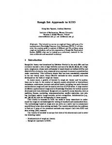
where tfij (term frequency, tf ) - number of times term tj occurs in document di , dfj (document frequency) - number of documents in the corpus in which term tj occurs. The factor log(N/dfj ) is called inverse document frequency (idf ) of term.
idf 1
0 1
df Figure 3.2: Plot of inverse document frequency (idf )
Document length normalization As documents in the collection can be of various length, there might be a case when large documents can dominates the document space (components of its vectors have significant larger values than other document), causes clustering to produce skewed, incorrect solution. To overcome this problem, length normalization is usually applied to document’s vector.
3.2.3. Similarity measure The distance or similarity between document vectors is quantified by various measures that have been developed (see [25]): 24
Document/T erm d1 d2 d3 d4 d5 d6
inf ormation 0.301 0.301 0.301 0 0 0
web 0 0 0 0.6021 0.301 0.301
query 0.4771 0 0 0 0 0.4771
retrieval 0.1761 0.1761 0.1761 0 0 0.1761
model 0 0.4771 0.4771 0 0 0
language 0.301 0.301 0.301 0 0 0
Figure 3.3: Example of TF*IDF weighting for document from 3.1. Weights of document vector are normalized by its length. Similarity Measure sim(X,Y)
Evaluation of Binary Term Vectors
Inner product
X
T
Evaluation of Weighted Term Vectors Pt
Y
i=1 xi
T
|X Y | 2 |X|+|Y |
Dice coefficient
Pt
Pt
i=1
T
|X Y | T |X|+|Y |−|X Y |
i=1
Pt xi yi qP i=1 P t t 2
T
Jaccard coefficient
xy
Pit i
i=1
x2 + i=1 i
|X Y | |X|1/2 +|Y |1/2
Cosine coefficient
2
· yi
Pt i=1
xi +
yi2
i=1
yi2
Pt xi yi Pt Pi=1 t 2
x2i +
i=1
yi −
i=1
xi yi
Table 3.3: Measures of vector similarity [25]. X, Y are document vectors. xi , yi are the weight (value) of the i-th component of vector. Due to its simplicity and intuitive interpretation, the cosine coefficient is most commonly used. When vectors representing documents are normalized by length, all above measures become quite similar to each other, ranging from 1 for identical documents, to 0 when there is nothing in common between documents.
3.2.4. Cluster representation The choice of cluster representation is essential for clustering algorithm. Good representation of cluster should take into account not only features of documents belonging to cluster, but also should adequately quantify the degree that each feature contribute to cluster contents. In vector space based approach, a cluster is usually represented as mean vector (the centroid) of cluster documents. Given a cluster Ck = {dk1 , dk2 , ..., dkm }, we can define the composite vector Dk of cluster as: X d = dk1 + dk2 + ... + dkm Dk = d∈Ck
and the cluster’s centroid as: ck =
dk1 + dk2 + ... + dkm Dk = |Ck | m 25
Sometimes, a median — an object (document) closest to the centroid – chosen to represent a cluster. While clusters need not necessarily to be represented as vectors in the same space as documents, doing so greatly simplifies the similarity (or distance) calculation between two clusters or between a cluster and a document (the same similarity measure for documents can be used).
3.3. Clustering algorithms Clustering algorithms based on vector space can be divided into two categories: hierarchical and partitioning.
3.3.1. Hierarchical algorithms
similarity
Agglomerative hierarchical clustering techniques starts with each object as a cluster, then iteratively merge two most similar clusters until only one cluster remains. As a result, the process creates a structure called dendogram - a tree which illustrates the merging process and intermediate clusters. With n objects there will be n − 1 merging steps.
Figure 3.4: Dendogram from a hierarchical clustering solution. By cutting off at specified level of dendogram a partitional solution is obtained. Algorithm 1 Agglomerative Hierarchical Clustering Input: set of objects: d1 , .., dn , similarity measures δ(di , dj ), i 6= j, i, j = 1..n 1: create initial clusters from given set objects, each object forming a cluster 2: for i = 1 to n − 1 do 3: find two most similar clusters and merge them creating a new cluster 4: end for By using different measure for similarity between clusters, diverse results can be achieved: single-linkage distance between two clusters is defined as the minimum distance between two objects, each coming from other cluster complete-linkage opposite from single-linkage, distance between two clusters is defined as the maximum distance between two objects, one from each cluster average-linkage the distance of two cluster is measured as an average of distances between all pairs of objects, where every pair consists of one object from each cluster 26
While complete-linkage algorithms are able to produce tight, compact clusters, more versatile solutions (clusters of different ”shapes” e.g. concentric or elongated) can be achieved with single-linkage (but it also may results in a ”chaining effect” – unnecessary merge due to existence of a chain of objects connecting two clusters [13]). In general, hierarchical algorithms are believed [13, 18] to achieve better clustering solutions than partitioning ones. However, more recently a comparison [31] shows that partitioning-based approach can be superior in document clustering. Because the computational complexity of agglomerative hierarchical algorithms is O(n2 log n) with memory consumption of O(n2 ) (for objects pair wise similarity matrix), where n – number of objects (documents), it is prohibited from application for large data set, where partitioning-based approach can be used.
3.3.2. Partitioning-based Partitioning algorithm divide the set of n objects into k clusters so that the objective criterion is optimized. Objective criterion is usually chosen to minimize (maximize) some similarity function(e.g. distance) between objects. The most popular partitioning-based algorithm are K-means and its variants. Algorithm 2 The K-means algorithm Input: number of cluster k, set of n objects 1: choose k objects arbitrarily to be representatives of k initial clusters 2: repeat 3: assign objects to closest cluster (in term of distance between given object and cluster’s representative) 4: recalculate clusters representatives 5: until no change or changes are small The computation requirement of K-means is relatively low — O(kn) (where k – number of cluster, n – number of documents) — hence it can be used for large collection of documents.
3.3.3. Optimization criteria In partitioning-based approaches, the clustering is usually leads by a global optimization criterion. Some most frequently used criteria, see [47], are:
Maximize internal similarity This criterion is based on the requirement that document within cluster must be similar to each other. Therefore, desired clustering solution should maximize the internal (within cluster) similarity between documents:
I1 =
k X r=1
nr (
1 n2r
X di ,dj ∈Cr
27
δ(di , dj ))
Maximize document-centroid similarity Maximizing aggregated similarity between each document and its cluster centroid, is a very common [7, 18] criterion for vector-space K-means algorithms: I2 =
k X X
δ(di , cr )
r=1 di ∈Cr
Minimize cluster-collection similarity Based on the premise that documents in different cluster should be differentiate as much as possible (i.e. documents share very few terms across clusters), one may come to a criterion to make centroid of clusters as mutually orthogonal as possible. However, [47] pointed out that for this criterion, trivial solutions could be achieved (e.g. k − 1 clusters, each contains a single document that share few terms with the rest, and the remaining documents are assigned to single cluster). Thus, a criterion, that aims to stretch out clusters by minimizing its similarity to central point (centroid) of the collection, has been proposed [47]: E1 =
k X
nr δ(Cr , C)
r=1
where C – centroid of the whole collection.
3.3.4. Hard vs. soft assignment For some application, especially with text, when assigning document to cluster, one may want to quantify how ”related” is the document to a cluster by associating real value – the membership degree. In document clustering, if we view clusters as a set of document sharing similar topic/theme, then it is natural that one document can be ”about” several topics anbd could be assigned to several clusters. The algorithm that uses the above notion is said to use fuzzy/soft assignment with overlapping clusters. In opposite, algorithm with hard assignment allows each document to belong only to one cluster without quantifying degree of the relation.
28
Chapter 4
Rough Sets and the Tolerance Rough Set Model Rough sets theory was originally developed [20, 14] as a tool for data analysis and classification. It has been successfully applied in various tasks, such as feature selection/extraction, rule synthesis and classification [14]. In this chapter we will present fundamental concepts of rough sets with illustrative examples. Some extensions of rough set are described, concentrating on the use of rough set to synthesize approximations of concepts from data.
4.1. Approximation of concept Consider a non-empty set of object U called the universe. Suppose we want to define a concept over universe of objects U . Let assume that our concept can be represented as subset X of U . The central point of rough set theory is the notion of set approximation: any set in U can be approximated by its lower and upper approximation.
Real world U X
Figure 4.1: Rough concept
4.1.1. Indiscernibility relation Originally [20], in order to define lower and upper approximation we need to introduce an indiscernibility relation: R ⊆ U ×U (where R can be any equivalence relation). For two objects x, y ∈ U , if xRy then we say that x and y are indiscernible from each other. The indiscernibility relation R induces a complete partition of universe U into equivalent classes [x]R , x ∈ U . 29
We define lower and upper approximation of set X, with regards to an approximation space denoted by A = (U, R), respectively as: LR (X) = {x ∈ U : [x]R ⊆ X} UR (X) = {x ∈ U : [x]R ∩ X 6= ∅}
(4.1)
Due to the fact that LR ⊆ X ⊆ UR , there is a special set BNR = UR − LR , called a boundary region of approximation. Intuitively,F lower approximation contains objects that certainly belong to our concept while upper approximation contains objects that may belong to our concept. Together, the pair (LR , UR ) constitutes for a rough approximation (or rough set) of concept X.
4.1.2. Rough membership Approximations can also be defined by mean of rough membership function [45]. Given rough membership function µX : U → [0, 1] of a set X ⊆ U , the rough approximation is defined as Lµ (X) = {x ∈ U : µ(x, X) = 1} Uµ (X) = {x ∈ U : µ(x, X) > 0} Note that, given rough membership function as µX (x, X) = equivalent to 4.1.
|[x]R ∩X| |[x]R | ,
(4.2) this definition is actually
4.1.3. Information Systems Until now, objects in the universe U were regarded as something abstract. In practice however, objects are usually real-world entities that are described by some information (most often denoted as inf (x) - information about object x). This is captured in a notion of information system. Formally, an information system is described as a pair: I = (U, A) where U - non-empty, finite set of objects called the universe, A - non-empty, finite set of attributes. For each attribute a ∈ A there is a corresponding evaluation function fa : U → Va , where Va is the value set of a. Intuitively any finite set of objects, in which objects are described by set of attributes can be perceived as an information system, e.g.: a group of people, where each person is characterized by their sex, age and occupation. The simplest form of information system is information table, a two dimensional array where rows correspond to objects and columns to attributes. For each object x ∈ U , the perceived information about x with w.r.t. set of attributes B ⊆ A is defined as B-information vector : infB (x) = {(a, fa (x)) : a ∈ B} Frequently, the information table is given in an extended form — with one additional distinguish column that contains a decision — which is referred as decision table. Example 1 Let consider an universe of hospital patients U = {p1 , p2 , p3 , p4 , p5 , p6 , p7 , p8 },given in a decision table 4.1 [21]. Patients are described by their symptoms of sickness. Let an equivalence relation R be defined by equality of two attributes Headache and Temperature (i.e. xRy ⇔ fHeadache (x) = fHeadache (y) ∧ fT emperature (x) = fT emperature (y)). This 30
Upper approximation of X
Lower approximation of X
Real world
Boundary region
U
P1 P5
P6
P4
p2 P3 P7
P8
X
Figure 4.2: Visualization of lower, upper approximation and boundary region of example set X in the universe U . Patient p1 p2 p3 p4 p5 p6 p7 p8
Headache yes yes yes no no no no no
Attributes Muscle pain yes yes yes yes no yes no yes
Temperature normal high very high normal high very high high very high
Decision Flu no yes yes no no yes yes no
Table 4.1: Example of an information system. equivalence relation induces a partition of U into classes {p1 }, {p2 }, {p3 }, {p4 }, {p5 , p7 }, {p6 , p8 }. We can see for example, that p5 and p7 are indiscernible with regards to relation R. Assuming that the concept X we want to describe is given here as a decision — if a patient has flu (X = {p2 , p3 , p6 , p7 }) — its approximation can be determined (Figure 4.2): LR (X) = {p2 , p3 } UR (X) = {p2 , p3 , p5 , p6 , p7 , p8 }
4.2. Generalized approximation spaces The classical rough set theory is based on equivalence relation that divides the universe of objects into disjoint classes. By definition, an equivalence relation R ⊆ U × U is required to be: 1. reflexive: xRx, for any x ∈ U 2. symmetric: xRy ⇒ yRx, for any x, y ∈ U 31
3. transitive: xRy ∧ yRz ⇒ xRz, for any x, y, z ∈ U Practically, for some applications, the requirement for equivalent relation has showed to be too strict. The nature of the concepts in many domains are imprecise and can be overlapped additionally. Example 2 Let us consider a collection of scientific documents and keywords describing those documents. It is clear that each document can have several keywords and a keyword can be associated with many documents. Thus, in the universe of documents, keywords can form overlapping classes. By relaxing the relation R to a tolerance relation, where transitivity property is not required, a generalized tolerance space is introduced by Skowron [2].
4.2.1. Definition Generalized approximation space is defined as a quadruple A = (U, I, ν, P ) where 1. U is a non-empty set of objects (an universe) 2. I : U → P(U ) is an uncertainty function (P(U ) - set of all subsets of U ) An uncertainty function I can be any function satisfying conditions: • x ∈ I(x) for x ∈ U • y ∈ I(x) ⇐⇒ x ∈ I(y) for any x, y ∈ U . thus the relation xRy ⇐⇒ y ∈ I(x) is a tolerance relation (i.e. reflexive, symmetric) and I(x) is a tolerance class of x. Intuitively, if we consider that objects x ∈ U are viewed through ”lenses” of available information inf (x) then I(x) is the set of objects in U that ”look” similar to x. 3. ν : P(U ) × P(U ) → [0, 1] is a vague inclusion function Vague inclusion ν is a kind of membership function (defined in 4) but extended to functions over P(U ) × P(U ) to measure degree of inclusion between two set. Vague inclusion can be any function ν : P(U ) × P(U ) → [0, 1] that is monotonic with respect to the second argument: Y ⊆ Z ⇒ ν(X, Y ) ≤ ν(X, Z)
for X, Y, Z ⊆ U
Together with uncertainty function I, vague inclusion function ν defines the rough membership function for x ∈ U, X ⊆ U : µI,ν (x, X) = ν(I(x), X) 4. P : I(U ) → {0, 1} is a structurality function The introduction of structurality function P : I(U ) → {0, 1} (I(U ) = {I(x) : x ∈ U }) allows us to enforce additional global conditions on sets I(x) considered to be approximated. In generation of approximations, only sets X ∈ I(U ) for which P (X) = 1 (referred as P-structural element in U ) are considered. For example, function Pα (X) = 1 ⇐⇒ |X|/|U | > α will discard all subsets that are relatively smaller than certain percentage (given by α) of U . 32
4.2.2. Approximations Approximations in A of any X ⊆ U are then defined as LA (X) = {x ∈ U : P (I(X)) = 1 ∧ ν(I(x), X) = 1}
(4.3)
UA (X) = {x ∈ U : P (I(X)) = 1 ∧ ν(I(x), X) > 0}
(4.4)
With given definition above, generalized approximation spaces can be used in any application where I, ν and P can be appropriately determined. Example 3 The standard rough set model (4.1) can be described as a particular case of generalized approximation. Let consider a quadruple A1 = (U, I, ν, P ) where • U – universe of objects • I(x) = [x]R where R ⊆ U × U is an indiscernibility relation • ν(X, Y ) =
|X∩Y | |Y |
where X, Y ⊆ U
• P (I(x)) = 1 for every x ∈ U With P (I(x)) = 1 for every x, the approximations can be simplified to: LA1 (X) = {x ∈ U : ν(I(x), X) = 1}
(4.5)
UA1 (X) = {x ∈ U : ν(I(x), X) > 0}
(4.6)
One can find that this is equivalent to the definition 4.2 where ν is a kind of rough membership function. Example 4 Variable Precision Rough Set [48] proposed a generalization of approximations by introducing a special non-decreasing function fβ : [0, 1] → [0, 1] (for 0 ≤ β < 0.5) satisfying properties: • fβ (t) = 0 ⇐⇒ 0 ≤ t ≤ β • fβ (t) = 1 ⇐⇒ 1 − β ≤ t ≤ 1 The generalized membership function called fβ -membership function is next defined as µ(fβ )(x, X) = fβ (t) = fβ (
|[x]R ∩ X| ) |[x]R |
The lower and upper approximations of a set X ⊆ U with respect to µ(fβ ) can be defined as follows: Lµ(fβ ) (X) = {x ∈ U : µ(x, X) = 1}
(4.7)
Uµ(fβ ) (X) = {x ∈ U : µ(x, X) > 0}
(4.8)
With β = 0 and fβ equal to identity on [0, 1] we have the case of classical rough set [20]. By varying the fβ , the extension introduced by variable precision rough set model can be viewed as a method of controlling the size and gradualness of boundary region. Variable Precision Rough Set can be also modelled as a generalized approximation space Aβ = (U, I, ν, P ) with 33
fβ(t) 1
variable precision rough set (β>0) β classical rough set (β=0) β
β
1
t
Figure 4.3: Example of fβ for variable precision rough set (β > 0) and classical rough set (β = 0) • U – universe of objects • I(x) = [x]R where R ⊆ U × U is an indiscernibility relation | • ν(X, Y ) = fβ ( |X∩Y |Y | ) where X, Y ⊆ U
• P (I(x)) = 1 for every x ∈ U
4.3. Tolerance Rough Set Model Tolerance Rough Set Model (TRSM) was developed [26, 34] as basis to model documents and terms in information retrieval, text mining, etc. With its ability to deal with vagueness and fuzziness, tolerance rough set seems to be promising tool to model relations between terms and documents. In many information retrieval problems, especially in document clustering, defining the relation(i.e. similarity or distance) between document-document, term-term or term-document is essential. In Vector Space Model, is has been noticed [34] that a single document is usually represented by relatively few terms1 . This results in zero-valued similarities which decreases quality of clustering. The application of TRSM in document clustering was proposed as a way to enrich document and cluster representation with the hope of increasing clustering performance. 1 In other words, number of non-zero values in document’s vector is much smaller than vector’s dimension – the number of all index terms
34
4.3.1. Tolerance space of terms Let D = {d1 , d2 , . . . , dN } be a set of document and T = {t1 , t2 , . . . , tM } set of index terms for D. With the adoption of Vector Space Model (3.2) each document di is represented by a weight vector [wi1 , wi2 , . . . , wiM ] where wij denoted the weight of term j in document i. In TRSM, the tolerance space is defined over a universe of all index terms U = T = {t1 , t2 , . . . , tM } The idea is to capture conceptually related index terms into classes. For this purpose, the tolerance relation R is determined as the co-occurrence of index terms in all documents from D. The choice of co-occurrence of index terms to define tolerance relation is motivated by its meaningful interpretation of the semantic relation in context of IR and its relatively simple and efficient computation. Tolerance class of term Let fD (ti , tj ) denotes the number of documents in D in which both terms ti and tj occurs. The uncertainty function I with regards to threshold θ is defined as Iθ (ti ) = {tj | fD (ti , tj ) ≥ θ} ∪ {ti } Clearly, the above function satisfies conditions of being reflexive: ti ∈ Iθ (ti ) and symmetric: tj ∈ Iθ (ti ) ⇐⇒ ti ∈ Iθ (tj ) for any ti , tj ∈ T . Thus, the tolerance relation I ⊆ T × T can be defined by means of function I: ti Itj ⇐⇒ tj ∈ Iθ (ti ) where Iθ (ti ) is the tolerance class of index term ti . In context of Information Retrieval, a tolerance class represents a concept that is characterized by terms it contains. By varying the threshold θ (e.g. relatively to the size of document collection), one can control the degree of relatedness of words in tolerance classes (or in other words the preciseness of the concept represented by a tolerance class). To measure degree of inclusion of one set in another, vague inclusion function is defined as |X ∩ Y | ν(X, Y ) = |X| It is clear that this function is monotonous with respect to the second argument. The membership function µ for ti ∈ T , X ⊆ T is then defined as µ(ti , X) = ν(Iθ (ti ), X) =
|Iθ (ti ) ∩ X| |Iθ (ti )|
With the assumption that the set of index terms T doesn’t change in the application, all tolerance classes of terms are considered as structural subsets: P (Iθ (ti )) = 1 for all ti ∈ T . Finally, the lower and upper approximations of any subset X ⊆ T can be determined — with the obtained tolerance R = (T, I, ν, P ) — respectively as LR (X) = {ti ∈ T | ν(Iθ (ti ), X) = 1} UR (X) = {ti ∈ T | ν(Iθ (ti ), X) > 0} One interpretations of the given approximations can be as follows: if we treat X as an concept described vaguely by index terms it contains, then UR (X) is the set of concepts that share some semantic meanings with X, while LR (X) is a ”core” concept of X. 35
Example 5 Consider an universe of unique terms extracted from a set of search result snippets returned from Google search engine for a ”famous”2 query: jaguar. Tolerance classes are generated for threshold θ = 9. It is interesting to observe that the generated classes do reveal different meanings of the word ”jaguar”: a cat, a car, a game console, an operating system and some more. Term Atari Mac onca club Panthera new information OS site Welcome X Cars
Tolerance class Atari, Jaguar Mac, Jaguar, OS, X onca, Jaguar, Panthera Jaguar,club onca, Jaguar, Panthera Jaguar, new Jaguar, information Mac,Jaguar, OS, X Jaguar, site Jaguar, Welcome Mac, Jaguar, OS, X Jaguar, Cars
Document frequency3 10 12 9 27 9 29 9 15 19 21 14 24
Table 4.2: Tolerance classes of terms generated from 200 snippets return by Google search engine for a query ”jaguar” with θ = 9; only non-trivial classes are shown.
4.3.2. Enriching document representation In standard Vector Space Model, a document is viewed as a bag of words/terms. This is articulated by assigning, non-zero weight values, in document’s vector, to terms that occurs in document. With TRSM, the aim is enrich representation of document by taking into consideration not only terms actually occurring document but also other related terms with similar meanings. A ”richer” representation of document can be acquired by representing document as set of tolerance classes of terms it contains. This is achieved by simply representing document with its upper approximation. Let di = {ti1 , ti2 , ..., tik } be a document in D and ti1 , ti2 , ..., tik ∈ T are index terms of di : UR (di ) = {ti ∈ T | ν(Iθ (ti ), di ) > 0}
4.3.3. Extended weighting scheme for upper approximation To assign weight values for document’s vector, the TF*IDF (see 3.2.2) weighting scheme is used. In order to employ approximations for document, the weighting scheme need to be extended to handle terms that occurs in document’s upper approximation but not in the document itself (or terms that occurs in the document but not in document’s lower 2
The word jaguar is frequently used as a test query in information retrieval (e.g. document classification, clustering, word disambiguation) because it is a polysemy (i.e. word that has several meanings) especially in the web: jaguar as a cat (panthera onca - http://dspace.dial.pipex.com/agarman/jaguar.htm); as an Jaguar car; it was a name for a game console made by Atari - http://www.atari-jaguar64.de, but also a codename for Apple’s newest operating system MacOS X - http://www.apple.com/macosx
36
approximation). The extended weighting scheme is defined as: (1 + log(fdi (tj )) ∗ log fDN(tj ) N
wij =
mintk ∈di wik ∗
log
fD (tj ) N fD (tj )
1+log
0
if tj ∈ di if tj inUR (di )\di if tj ∈ / inUR (di )
(where wij is the weight for term tj in document di ). The extension ensures that each terms occurring in upper approximation of di but not in di , has a weight smaller than the weight of any terms in di . Normalization by vector’s length is then applied to all document vectors: wij wij = qP 2 tk ∈di (wij ) TITLE DESCRIPTION
EconPapers: Rough sets bankruptcy prediction models versus auditor Rough sets bankruptcy prediction models versus auditor signalling rates. Journal of Forecasting, 2003, vol. 22, issue 8, pages 569-586. Thomas E. McKee. ... Document vector original using upper approximation Term Weight Term Weight auditor 0.567 auditor 0.564 bankruptcy 0.4218 bankruptcy 0.4196 signalling 0.2835 signalling 0.282 EconPapers 0.2835 EconPapers 0.282 rates 0.2835 rates 0.282 versus 0.223 versus 0.2218 issue 0.223 issue 0.2218 Journal 0.223 Journal 0.2218 MODEL 0.223 MODEL 0.2218 prediction 0.1772 prediction 0.1762 Vol 0.1709 Vol 0.1699 applications 0.0809 Computing 0.0643
Table 4.3: Example snippet and its upper approximation.
37
Chapter 5
The Tolerance Rough Set clustering algorithm for search results This chapter starts with the introduction of document clustering algorithms based on Tolerance Rough Set Model. The chapter continues by outlining special characteristic of data which is search results. An adaptation of TRSM-based algorithm for web search results clustering is next proposed and described in details.
5.1. Document clustering algorithms based on TRSM With the introduction of Tolerance Rough Set Model in [26], several document clustering algorithms based on that model was also introduced [26, 34]. The main novelty that TRSM brings into clustering algorithms are the way of representing clusters and document.
5.1.1. Cluster representation As discussed earlier in 3.2.4, determining cluster representation is very important factor in partitioning-based clustering. Frequently, cluster is represented as a mean or median of all documents it contains. Sometime however, a representation not based on vector is needed as cluster description is directly derived from its representation. For example, cluster can be represented by most ”distinctive” terms from cluster’s documents (e.g. most frequent terms; or frequent terms in clusters but infrequent globally). In [34], an approach to construct a polythetic representation is presented. Let Rk denotes a representative for cluster k. The aim is to construct a set of index terms Rk representing cluster Ck so that: • each document di in Ck share some or many terms with Rk • terms in Rk occurs in most documents in Ck • terms in Rk needs not to be contained by every document in Ck The weighting for terms tj in Rk is calculated as an averaged weight of all occurrences in documents of Ck : P di ∈Ck wij wkj = |{di ∈ Ck | tj ∈ di }| 39
Algorithm 3 Determine cluster representatives 1: Rk = ∅ 2: for all di ∈ Ck and tj ∈ di do 3: if fCk (tj )/|Ck | > σ then 4: Rk = Rk ∪ tj 5: end if 6: end for 7: if di ∈ Ck and di ∩ Rk = ∅ then 8: Rk = Rk ∪ argmaxtj ∈di wij 9: end if Let fCk (tJ ) be the number of documents in Ck that contain tj . The above assumptions lead to following rules to create cluster representatives: To the initially empty representative set, terms that occur frequent enough (controlled by threshold σ) in documents within cluster are added. After this phase, for each document that is not yet ”represented” in representative set (i.e. document shares no terms with Rk ), the strongest/heaviest term from that document is added to the cluster representatives.
5.1.2. TRSM-based non-hierarchical clustering algorithm The non-hierarchical document clustering algorithm based on TRSM is a variation of a Kmeans clustering algorithm (3.3.2) with overlapping clusters. The modifications introduced are: • use of document’s upper approximation when calculating document-cluster and documentdocument similarity • documents are soft-assigned to cluster with associated membership value • use nearest-neighbor to assign unclassified documents to cluster The use of upper approximation in similarity calculation to reduce the number of zerovalued similarities is the main advantage main advantage TRSM-based algorithms claimed to have over traditional approaches. This allows the situation, in which two document are similar (i.e. have non-zero similarity) although they do not share any terms.
5.1.3. TRSM-based hierarchical clustering algorithm A hierarchical agglomerative clustering algorithm based on TRSM was proposed in [26]. It utilizes upper approximation to calculate cluster similarities in the merging step. Both presented clustering algorithms were evaluated with standard test collections and has shown some success [26, 34].
5.2. Clustering search results Despite being derived from document clustering, methods for clustering web search results differ from its ancestors on numerous aspects. Most notably, document clustering algorithms are designed to works on relatively large collection of full-text document (or sometimes document abstract). In opposite, the algorithm for web search results clustering is supposed to works on moderate size (several hundreds elements) set of text snippets (with length of 40
Algorithm 4 TRSM-based non-hierarchical clustering algorithm Input: D – set of N documents, K – number of clusters Output: K overlapping clusters of documents from D with associated membership value 1: Randomly select K document from D to serve as K initial cluster C1 , C2 , ..., CK . Each chosen document also forms cluster representative R1 , R2 , ..., RK . 2: repeat 3: for each di ∈ D do 4: for each cluster Ck , k = 1, .., K do 5: calculate the similarity between document’s upper approximation and the cluster representatives S(UR (di ), Rk ) 6: if S(UR (di ), Rk ) > δ then 7: assign di to Ck with the similarity taken as cluster membership: m(di , Ck ) = S(UR (di ), Rk ) 8: end if 9: end for 10: end for 11: for each cluster Ck do 12: re-determine cluster representative Rk 13: end for 14: until the is little or no change in cluster membership 15: for each unclassified document du (document has not been assigned to any cluster) do 16: let N N (du ) denotes nearest neighbor (with non-zero similarity) of du 17: assign du to cluster Ck that contains N N (du ) 18: calculate membership m(du , Ck ) = m(N N (du ), Ck ) · S(UR (du ), UR (N N (du ))) 19: end for 20: for each cluster Ck do 21: re-determine cluster representative Rk 22: end for
Algorithm 5 TRSM-based hierarchial agglomerative clustering algorithm Input: D – set of N documents, S – similarity measure Output: hierarchical structure H of clusters Ck 1: Initially, each document di ∈ D form a one document cluster Ci = di . H = C1 , C2 , ..., CN . 2: while there is more than one cluster, |H| > 1 do 3: find two most similar clusters in terms of their representative upper approximation (Cn1 , Cn2 ) = argmax(Cu ,Cv )∈H×H S(UR (Ru ), UR (Rv )) 4: merge two cluster Cn1 ∪ Cn2 = Ck and let H = (H {Cn1 , Cn2 }) ∪ {Ck } 5: end while
41
10-20 words). In document clustering, the main emphasis is put on the quality of clusters and the scalability to large number of documents, as it is usually used to process the whole document collection (e.g. for document retrieval on clustered collection). For web search results clustering, apart from delivering good quality clusters, it is also required to produce meaningful, concise description for cluster. Additionally, the algorithm must be extremely fast to process results on-line (as post-processing search results before delivered to the user) and scale with the increase of user requests (e.g. measures as number of processed requests per specified amount of time). document clustering full-text documents (or document abstract) off-line processing of large collection cluster quality scalability with number of documents
web search results clustering short text snippets on-line processing of moderate size set cluster quality + cluster description meaningfulness scalability with number of user requests
Table 5.1: Comparison between document clustering and web search results clustering
5.3. The TRC algorithm The Tolerance Rough Clustering algorithm is based primarily on the K-means algorithm presented in (5.1.2) [34]. By adapting K-means clustering method, the algorithm remain relatively quick (which is essential for on-line results post-processing, see 2.3) while still maintaining good clusters quality. The usage of Tolerance Space and upper approximation to enrich inter-document and document-cluster relation allows the algorithm to discover subtle similarities not detected otherwise. As it has been mentioned, in search results clustering, the proper labelling of cluster is as important as cluster contents quality. Since the use of phrases in cluster label has been proven [44, 19] to be more effective than single words, TRC algorithm utilize n-gram of words (phrases) retrieved from documents inside cluster as candidates for cluster description.
documents preprocessing
documents representation building
tolerance class generation
clustering
Figure 5.1: Phases of TRC algorithm The TRC algorithm is composed from five phases (depicted in 5.1): 1. documents preprocessing 2. documents representation building 3. tolerance class generation 4. clustering 5. cluster labelling 42
cluster labelling
5.3.1. Preprocessing It is widely known [16] that preprocessing text data before feeding it into clustering algorithm is essentials and can have great impact on algorithm performance. In TRC, several preprocessing steps are performed on snippets: Text cleansing In this step, text content of snippet is cleaned from unusable terms such as: • non-letter characters like , $, # • HTML-related tags (e.g.=
, ) and entities (e.g. &, ") Stemming A version of Porter’s stemmer [23] is used in this step to remove prefixes and suffixes, normalizing terms to its root form. This process can greatly reduce vocabulary of the collection without much semantic loss. The stemmed terms are linked to its original form, which are preserved to be used in subsequent phases (i.e. labels generation). Stop-words elimination A stop-word itself doesn’t bring any semantic meanings but in connection with other words can form meaningful phrases. Therefore, terms that occur in stop-word list are specially marked to be ignored from document index terms, but not removed (so it can uses in phrases extraction in label generation phase). Due to special nature of web document, some words like ”web”, ”http”, ”site” appear very frequently, thus a stop-word list adapted to web vocabulary from [39] is used.
5.3.2. Document corpus building As TRC utilizes Vector Space Model for creating document-term matrix representing documents. Index terms selection Index terms are selected from all unique stemmed terms after stop-words elimination and with regards to the following rules: • digits and terms shorter than 2 characters are ignored • terms contained in the query are ignored (as we are operating on the top search results for a query, terms from query will occurs in almost every snippet) • Minimum Document Frequency filtering - term that occurs in less given threshold (e..g less than 2 snippets) are ignored as they will doubly contributes to document characterization Selected index terms used to characterize documents are enumerated and a document-term frequency matrix is built. Let N be a number of document – search results snippets, and M is the number of selected index terms. The document-term frequency matrix is defined as follows: T F = [tfi,j ]N ×M 43
where tfi,j — number of occurrences of term j in document j. Each row T F [i] of T F matrix is a characterization of the i-th document by means of term frequencies. Term weighting The TF*IDF term weighting scheme is applied for document-term matrix to create documentterm weight matrix: W = [wi,j ]N ×M where wi,j — weight of term j in i-th document. Each row W [i] in the W matrix represents a characterization of the i-th document by means of weighted terms.
5.3.3. Tolerance class generation M
N
documen-term frequency matrix
M
N
1
term occurrence binary matrix
2
M term tolerance matrix M
M
3
term co-occurrence matrix M
Figure 5.2: Process of generating tolerance classes The goal of the tolerance class generation is to determine for each term, set of its related terms with regards to the tolerance relation – the tolerance class. This phase exists for computation optimization purpose, it ensures that the calculation of the upper approximation for a set of terms can be done quickly. Let define term co-occurrence matrix as T C = [tcx,y ]M ×M where tcx,y is a co-occurrence frequency of two terms x, y — number of documents in the collection in which terms x and y both occur. Let tolerance relation R between terms be defined as xRy ⇐⇒ tcx,y > θ where θ is called co-occurrence threshold. Having term co-occurrence matrix calculated we can define tolerance relation with different granularity by varying co-occurrence threshold. The computation cost of step 1 is O(N × M ), step 2 and 3 are both O(M 2 ), altogether is O(N × M 2 ). 44
Algorithm 6 Tolerance class generation (Figure 5.2) Input: T F – document-term frequency matrix, θ – co-occurrence threshold Output: T OL – term tolerance binary matrix defining tolerance classes of term 1: Calculate a binary occurrence matrix OC based on document-term frequency matrix T F as follows: OC = [oci,j ]N ×M where (
oci,j =
1 if tfi,j > 0 0 otherwise
Each column in OC is a bit vector representing term occurrence pattern in a document — bit is set if term occurs in a document. 2: Construct term co-occurrence matrix COC = [cocx,y ]M ×M as follows: for each pair of term x, y represented as pair of columns OC[x], OC[y] – bit vectors – in the OC matrix cocx,y = card(OC x ANDOC y ) where AND is a binary AND between bit vectors and card return cardinality – number of bits set – of a bit vector. bocx,y is the co-occurrence frequency of term x and y 1 . 3: given a co-occurrence threshold θ, a term tolerance binary matrix T OL = [tolx,y ]M ×M ] can be easily constructed by filtering out cells with values smaller than threshold θ : (
tolx,y =
1 if cocx,y ≥ θ 0 othewise
Each row in the resulting matrix forms a bit vector defining a tolerance class for given term: tolx,y is set if term x and y are in tolerance relation.
5.3.4. K-means clustering TRC adapts a variation of K-means algorithm for creating groups of similar snippets. Several main steps of the algorithm are described below (see pseudo-code in Algorithm 7): Initial cluster forming Selected documents serve as initial cluster representatives R1 , R2 , ..., RK . Stop condition The fact that the clustering algorithm is used as a post-retrieval2 process puts a strict constraint on execution time, as users are not willing to wait more than a few seconds for a response. We decided to set a limit of maximum number of iteration for the K-means algorithm. Due to the nature of quick convergence of K-means algorithm, this limit allows us to reduce the response time of the clustering engine with insignificant lost in clustering quality. Determining cluster representatives Cluster representatives is determined as described in 5.1.1 2 Results returned from search engine is processed on-the-fly by the clustering algorithm and presented to the user
45
Algorithm 7 Clustering phase of TRC algorithm Input: D – set of N documents, K – number of clusters, δ – cluster similarity threshold Output: K overlapping clusters of documents from D with associated membership value 1: Randomly select K document from D to serve as K initial cluster C1 , C2 , ..., CK . 2: repeat 3: for each di ∈ D do 4: for each cluster Ck , k = 1, .., K do 5: calculate the similarity between document’s upper approximation and the cluster representatives S(UR (di ), Rk ) 6: if S(UR (di ), Rk ) > δ then 7: assign di to Ck with the similarity taken as cluster membership: m(di , Ck ) = S(UR (di ), Rk ) 8: end if 9: end for 10: end for 11: for each cluster Ck do 12: determine_cluster_representatives(Rk ) 13: end for 14: until stop condition() 15: post-process unassigned documents 16: if necessary determine_cluster_representatives(Rk ) for changed clusters Ck Nearest neighbor assignment As a result of the restriction set by cluster similarity threshold, after all iterations there may exists document that has not been assigned to any cluster. In TRC, there are two possible options: • create a special ”Others” cluster with unassigned documents as proposed by [19] • assigns these documents to their nearest cluster For the later options, we have decided to assign document to its nearest neighbor’s cluster. Algorithm 8 Assignment of document to its nearest neighbor’s cluster for each unassigned document du do find the nearest neighbor document N N (du ) with non-zero similarity amongst clusters which N N (du ) belongs to; choose the one Ck that N N (du ) has strongest membership with assign du to Ck and calculate its cluster membership as m(du , Ck ) = m(N N (du ), Ck ) · S(UR (du ), UR (N N (du ))) end for
5.3.5. Cluster label generation As already pointed out, when evaluating clustering algorithms for search results, the quality of cluster label is as much important as the quality of the cluster itself. For labelling cluster we have decided to employs phrases because of its high descriptive power [44, 19]. We have adapted an algorithm for n-gram generation from [28] to extract phrases from contents of each 46
cluster. Most descriptive phrases are chosen to serve as labels for cluster. Descriptiveness of phrases is evaluated by taking into consideration following criteria: • frequency of the phrase in the whole collection • frequency of the phrase inside a cluster • length of the phrase, measured as number of words it is made from Following the intuition of TD*IDF scheme, we hypothesize that phrases that are relatively infrequent in the whole collection but occurs frequently in clusters will be good candidate for cluster’s label. We also prefer long phrases over shorter one.
5.4. Implementation The TRC algorithm was implemented entirely in Java programming language, as a component within the Carrot2 framework. The choice of Java as an implementation language was motivated by many reasons. Java is a platform-independent, object-oriented language that encourage good software development practices by enforcing the usage of interfaces and proper organization of source code. There are numerous open-source libraries of software components necessary when developing clustering engines (e.g. XML processing, visualization, Natural Language Processing), available for free.
5.4.1. Carrot2 Framework Carrot2 is an open-source, data processing framework developed by Dawid Weiss [37]. It enables and ease experimentation of processing and visualization of search results. The Carrot2 architecture is based on a set of loosely-coupled but cooperating components that exchanges information with each other using XML messages. Standard components in the
Figure 5.3: Data flow in Carrot2 framework Carrot2 framework are based on simple request-response paradigm – for a request sent to the component in a response is generated – supervised by special controller component. The data exchange between components is based on XML format and coordinated by the Carrot2 Controller (see 5.3). The controller serves also as an interface for external system as it accepts user’s query request and returns processed, formatted results. 47
Components in the Carrot2 framework can be classified into three types: input component serves as a data source. A typical input component could be a wrapper for search engine, that takes a user query, submit to the search engine and fetch the results returned for further processing. filter component is used to transform one data set to another. An example of filter component could be stemming, stop-word removal or the whole clustering algorithm (as it is the case in this thesis). output component’s role is to turn incoming data to a presentable format for the users. For instance, output could transform XML data to HTML format so that it can be viewed in standard web browser.
5.4.2. TRC as a Carrot2 filter component The TRC algorithm was implemented as a filter component within the Carrot2 framework. The use of Carrot2 framework instead of implementing the whole system by oneself was due to the following reasons: • Carrot2 provide a powerful yet relatively simple framework designed specially with intention to serve as experimentation environment for clustering search results algorithms • at the time writing, the Carrot2 framework has provided ready-to-use wrapper components as well as a visualization interface • Carrot2 is tested and has proven itself to be reliable data processing framework as several clustering algorithms [39, 19, 40] has been implemented with success
48
Search engine Search results
Wrapper
Preprocessing
Clustering engine Label generation
Carrot2 components
... Clustering component
Stop-words removal
Stemming
Snippets
Cluster-results visualization
Carrot2 framework Browser Figure 5.4: TRC as a filtering components within Carrot2 framework.
49
Chapter 6
Evaluation, experiments, comparisons This chapter presents an evaluation of our proposed TRC algorithm. We start by describing current methods for evaluation document clustering, continuing with detailed description of evaluation approach that we have adapted and its outcomes. Our evaluation concentrates on following goals: 1. investigating if the document’s enrichment offered by tolerance space can improve cluster’s quality 2. compare clustering quality of TRC with other search results clustering algorithm
6.1. Current evaluation methods When looking at current approaches to evaluation for document clustering, one can observes two categories of methods.
6.1.1. Ground truth First category of evaluation methods is originated from Information Retrieval domain and is based on a ground truth set[30] — a reference set of documents with accompanying information about relevance (documents are pre-classified as relevant or not, or assigned a relevance degree) or partition (documents are assigned to pre-identified groups). The tested algorithm is executed with those input documents and the results compared with original classification or partition. Methods of evaluation then vary on how to prepare the test collection and what metrics are used to measure the quality of results. Precision-Recall Precision and recall are standard measures used for evaluating quality of information retrieval systems. Let D be a set of documents, Q ⊆ D set of all relevant documents, A set of documents retrieved by system and AQ = A ∩ Q set of relevant document retrieved by system. The precision p and recall r can be defined as follows [25]: p=
|AQ | |A|
51
|AQ | |Q| An ideal solution would be a system producing results with both precision and recall equals 1, but in practice algorithms are trying first to achieve as much precision as possible while maintaining reasonable recall. With the assumption that resulting cluster is ordered in some way (e.g. in [11] users are assumed to be able to locate the ”best” clusters), these measures can be adapted for evaluation clustering search results [44]. r=
Merge-then-cluster For document clustering, a useful evaluation technique is to take documents from different sources/domain (so that it is inherently about different topics) and merge them together to create a test collection. The performance of clustering algorithm is then measured based on comparison of the resulting clusters and original classes of documents. A common metric used is the entropy measure, which considers the distribution of various classes of documents amongst clusters. Entropy for a clustering solution, as in [47] is defined as: E=
k X nr r=1
where E(Cr ) = −
n
E(Cr )
q 1 X nir ni log r log q i=1 nr nr
and Cr is a cluster with size nr , q – number of document classes, nir – number of documents of i-th class that was assigned to cluster Cr . Methods of this category depend largely on quality and availability of test collection. For example, document collections with pre-classification performed by expert may be debatable as there is always some subjectivity involves, while clustering document from different sources could reveal the topic sharing between document originally not related. The main advantage of ground-truth methods is that once a test collection is available, it can be automatically performed, thus the algorithm can be easily tested with various parameters and/or compared with other algorithms.
6.1.2. User feedback As many applications of document clustering were developed with purpose to help users in various information task, user evaluation seems to be natural way to assess its usefulness. User evaluation methods can be based on direct reports from the users (e.g. survey) or on automatic analysis of user interaction with the system (e.g. log analysis, web usage mining). An extensive example of user evaluation is presented in [44] and minor attempts were done in [19][40]. The problem with user evaluation is that for providing statistically significant results it must be done on large scale. Collecting surveys from a large number of users or attracting users to use an experimental system for a reasonable period of time (so that extensive log could be gathered) is a non-trivial task.
6.2. Our evaluation For limited time and resources assigned for this thesis, we could not perform a significant user evaluation. Also the lack of standard collection of web snippets has prevented us from doing 52
extensive evaluation. Instead, we have carried only an expert (by ourselves) evaluation of the proposed algorithm in a small own-authored set of test data and compared our solution with other approaches based on several examples.
6.3. Test data collection Due to aforementioned lacks of standard collection for testing web search results clustering, we had to build a small test collection. For this purpose, we have defined a set of queries for which results were collected from major search engine Google [10] to form test data collection.
6.3.1. Test queries The test set is composed from queries representing subjects of various degree of specificity, in order to test algorithm behavior on data with different vocabulary characteristic. The first three queries represent very general concepts and are frequently used as a test by authors [44, 39, 19, 40] of search results clustering algorithm. Next three queries are more specific subjects but broad enough to have interesting subclasses. Last three queries are about relatively specific topics and were chosen to test algorithm on highly cohesive vocabulary. In Table 6.1, figures in the second column are the approximated number of results for a queries retrieved from Google. Looking at these figures gives us some additional intuition about generality (or specificity) of concepts represented by query, or just popularity of each subject on the Web. Query java clinton jaguar ”data mining” wifi clustering voip ”rough sets” ”search results clustering”
Results count1 23400000 4270000 2580000 1080000 864000 810000 916000 748 105
Specificity2 low low low medium medium medium high high high
Table 6.1: Queries used to generate test collection.
6.3.2. Data characteristic Table 6.2 shows some statistics of snippets collection retrieved from Google search engine for set of test queries. Both stemming and stop-word list were used to filter out unnecessary terms. Additionally Minimum Document Frequency filter was used to remove terms that occurs in less than 2 documents. Thus, the indexing vocabulary could be reduced by about 70% (see Table 6.3). On average a snippets is indexed by 6 to 10 terms, which is about 2-3% of total vocabulary. This is very specific for search results snippets and in consequences the representing vectors are very sparse. Worth noticed in the results of term filtering, some document may be left represented by none terms. In our test collection, this happens in case of several queries (see last column of Table 6.2). This is because all terms in document were too specific and existed only in this document. Therefore, they were removed by Minimum Document Frequency filter. We can view these documents as an outlier area. 53
Query java clinton jaguar ”data mining” wifi clustering voip ”rough sets” ”search results clustering”
Snippets 200 200 200 200 200 195 200 146 68
Terms 332 337 339 319 340 319 355 244 149
Terms per snippet Average Min Max 7.28 0 15 7.305 0 13 6.595 0 13 8.815 0 16 6.915 1 19 7.456 0 16 8.235 0 17 9.089 1 18 12.279 2 19
Zero-terms snippets 1 3 3 2 0 2 5 0 0
Table 6.2: Characteristic of snippets retrieved from Google for defined queries.
6.3.3. Effects of terms filtering
Figure 6.1: Effects of terms filtering on number of terms (data from Table 6.3) The effects of different filtering techniques on vocabulary (i.e. number of unique terms) are showed in an example (see Table 6.3) of 200 snippets returned by search engine for query ”data mining”. Figures from the last column of Table 6.3 shows the percentage of vocabulary terms that has been reduced by the usage of both stemming and stop-word list (numbers in 1-st data column) in comparison with a situation when no stemming and stop-word list were used (figures from 4-th data column). The usage of stemming and stop-word list results in about 20% reduction of vocabulary (see the last column of Table 6.3). More notably however, is fact that the simple Minimum Document Frequency (MDF) filter which removes terms occurring in less than given threshold of documents (2 in this case) could reduce vocabulary by nearly 70% (compare the 1-st data row with the 2-nd data row in Table 6.3), thus greatly improves computation performance. When looking at data in the Table 6.3, an interesting observation can be made. In case when no additional filter is used, with changing combination of stemming/stop-word, there is a consecutive increase in number of terms (Table 6.3, data in the second row, moving from left to right). When MDF filter is used (Table 6.3, first row), 54
in contrast, there is a strong decline in number of terms when moving from combination stemming/no stop-word to no stemming/stop-word. We will explain this on the following example Example 6 Let consider following words: ”computer”, ”computers”, ”computing”, ”compute” and let assume that each occurs in exactly one document in the collection. The application of stemming brings all these words into a common form ”comput” which will have a document frequency of 4 and will remain untouched after MDF filter. When no stemming is applied, document frequency of each of these words are 1 and they may be removed by MDF filter with threshold 2 (only terms occurring in 2 or more documents are preserved).
MDF filter no filter % reduced
stemming stopword 319 971 67,14%
stemming no stopword 386 1074 64,05%
no stemming stopword 323 1142 71,71%
no stemming no stopword 389 1246 68,78%
% reduced 17,99% 22,07% 74,39%3
Table 6.3: Number of unique terms for 200 snippets retrieved for query ”data mining” and the effects of stemming, stop-words and MDF filtering on collection’s vocabulary.
6.4. Tolerance classes generation For testing the effects of varying co-occurrence threshold on generation of tolerance classes we have defined the two measures: number of tolerance classes and tolerance richness. For precise definition of these measures, we will introduce the following metaphor: • lets each index term ti is treated as a node vi in a graph G • edges in graph G represent the tolerance relation between terms: if terms ti1 , ti2 are in tolerance relation then its equivalent nodes vi1 , vi2 in graph G are connected with edge ei1,i2 • self-edges – edge connecting nodes with its self (this can happen as with 4.3.1 each terms is tolerance relation with itself) – are ignored number of tolerance classes is a number of terms with non-trivial tolerance class – classes with size ≥ 2 (i.e. number of nodes that have edges in graph G) tolerance richness is a number of edges in graph G. This measures the richness of the tolerance relation and also reflects the total size of all tolerance classes.
6.4.1. Size and richness Tolerance class generation was carried on sets of 200 snippets for test queries (see Table 6.2). The number of tolerance classes generated stabilizes pretty quickly (see Figure 6.2, 6.3) with the increase of co-occurrence threshold. The similarity can be observed for tolerance richness (see Figure 6.4, 6.5), also starting to stabilize after certain threshold (ranging in 4-8, varies from query). This confirms believes that the co-occurrence relation represented by tolerance classes of term is backed by existing underlying relation between terms. Some backing examples of generated tolerance classes are in Table 6.4 and 6.5. 55
Figure 6.2: Number of tolerance classes with various co-occurrence thresholds
Figure 6.3: The change in number of tolerance classes while varying co-occurrence threshold
6.5. Upper approximation enrichment In this section, we will try to answer the questions whether the usage of upper approximation can enrich document representation, and what effect will it have on inter-document 56
Figure 6.4: Number of connections between terms in tolerance classes (total size of all tolerance classes)
Figure 6.5: The change in number of connections between terms in tolerance classes (change in total size of all tolerance classes) while varying cooccurrence threshold
57
Term Intelligence Discovery SIGKDD Machine studies White case Paper services statistical Learning Business KDD Software Knowledge International webcasts Conference Workshop ACM
Tolerance class Intelligence, Business Discovery, SIGKDD, KDD, Knowledge, International, Conference, ACM Discovery, SIGKDD, Knowledge, ACM Machine, Learning studies, White, case, Paper, webcasts studies, White, case, Paper, webcasts studies, White, case, Paper, webcasts studies, White, case, Paper, webcasts services, Software statistical, Learning Machine, statistical, Learning Intelligence, Business Discovery, KDD, Knowledge, International services, Software Discovery, SIGKDD, KDD, Knowledge, International, Conference, ACM Discovery, KDD, Knowledge, International, Conference, Workshop studies, White, case, Paper, webcasts Discovery, Knowledge, International, Conference International, Workshop Discovery, SIGKDD, Knowledge, ACM
Table 6.4: Tolerance classes generated from snippets of query ”data mining” with cooccurrence threshold set to 6. Term Computing Discovery Polkowski data Skowron Current knowledge Trends Granular Andrzej International mining Conferences RSCTC Workshop Lech applications
Tolerance class Computing, data, Current, Trends, Granular, International, mining, Conferences, RSCTC Discovery, Polkowski, knowledge, Lech, applications Discovery, Polkowski, Skowron, knowledge, Lech, applications Computing, data, Granular, mining Polkowski, Skowron, Andrzej Computing, Current, Trends, International, Conferences, RSCTC Discovery, Polkowski, knowledge, Lech, applications Computing, Current, Trends, International, Conferences, RSCTC Computing, data, Granular, mining Skowron, Andrzej Computing, Current, Trends, International, Conferences, Workshop Computing, data, Granular, mining Computing, Current, Trends, International, Conferences Computing, Current, Trends, RSCTC International, Workshop Discovery, Polkowski, knowledge, Lech, applications Discovery, Polkowski, knowledge, Lech, applications
Table 6.5: Tolerance classes generated from snippets of query ”rough sets” with co-occurrence threshold set to 7. similarities. Most concepts like document representation, tolerance classes, inter-document similarities, are represented in our system as a matrix. Therefore, we want to examine the matrix of underlying concepts with and without upper approximation in use. Generally, we are interested in the some kind of ”richness” of these matrices. For evaluating matrix’s richness, let introduce the cardinality measure for matrix: cardthreshold − number of matrix’s entries, that values are greater than given threshold 58
(for threshold = 0 it is equivalent to number of non-zero entries). For each concept that we want to investigate, it equivalent matrix is constructed, firstly without using upper approximation and later utilizing upper approximation with various cooccurrence thresholds. The above defined cardinality is calculated for each of the constructed matrix and compared. Let M denotes a matrix representing investigated concept without usage of upper approximation and MU denotes the matrix of the same concept but utilizing upper approximation. The cardinality with specified threshold t for these matrices is denoted cardt (M ), cardt (MU ) adequately. The relative improvement of matrix’s richness brought in by upper approximation can be measured as follows: relative richness improvement =
cardt (MU ) − cardt (M ) cardt (M )
6.5.1. Upper approximation of document representation We want to measure how much ”richer” is the document representation when upper approximation is used, compared to the original representation. Recall from Section 3.2 that documents are represented in vectors, together composing a document-term matrix. The richness of document-term matrix can be measured as number of non-zero entries (cardt with t = 0). The cardinality for the document-term matrix without and with upper approximation was calculated using various co-occurrence thresholds and presented in figure 6.6. The improvement shown in figure 6.6 is very similar in nature to that of tolerance classes (see Figure 6.2), It is characterized with strong decrease at the beginning and quick stabilization starting from co-occurrence threshold of 5. Figure 6.7 shows relative improvement of document-term matrix’s richness when upper approximation is applied with co-occurrence threshold of 5. This is a clear proof that upper approximation can significantly improve the richness of document representation for all tested queries.
6.5.2. Inter-document similarity Similarity between two documents — inter-document similarity — calculated using one of defined measure (see 3.2.3) quantifies the relatedness between documents. The main purpose upper approximation is to enhance the association between documents (i.e. increase the similarity between related documents). To measure that enhancement, we have to examine inter-document similarity for all pairs of documents in the collection. Inter-document similarity for the whole document collections can be represented in a squared, symmetrical matrix called inter-document similarity matrix. The inter-document similarity matrix can be defined as: IDS = [si,j ]N ×N where si,j is the similarity between document i and j in the collections of N documents. si,j usually has value between 0 and 1 depending on used similarity measure. In experiments below, the cosine coefficient (see Section 3.2.3) was used. Because the inter-document similarity matrix is symmetrical and the entries in the diagonal (self similarities) are interested, in calculation of matrix’s cardinality only values in the upper diagonal were considered. We calculated inter-document similarity matrix for all snippets collection (as defined in 6.2) with standard document representation and the one using upper approximation. The cardinality for different threshold t (t = 0, 0.33, 0.5, 0.67) measured for these matrices is presented in Figures 6.8-6.11. 59
Figure 6.6: Relative improvement of document-term matrix when using upper approximation.
Figure 6.7: Relative improvement of document-term matrix when using upper approximation with co-occurrence threshold = 5. Figures 6.8 - 6.11 shows plot of relative improvement of inter-document similarity for similarity threshold 0, 0.33, 0.5, 0.67 with increasing co-occurrence threshold. From these 60
Figure 6.8: Relative improvement of inter-document similarity matrix measure for t = 0
Figure 6.9: Relative improvement of inter-document similarity matrix measure for t = 0.33 figures, it can be observed that the enrichment of upper approximation had indeed improved inter-document similarities for all queries. The level of improvement varies with different queries depending on the co-occurrence threshold. Some queries like ”java”, ”clinton”, ”voip”, 61
Figure 6.10: Relative improvement of inter-document similarity matrix measure for t = 0.5
Figure 6.11: Relative improvement of inter-document similarity matrix measure for t = 0.67 achieved significantly better level of improvement than others (”jaguar”, ”clustering”). This is showed in figure 6.12 where we set co-occurrence threshold at 5 and plot relative improvement for various thresholds t. It is promising that improvement has happened in all range of values. 62
Not only low-range values (e.g. increased number of non-zero entries) but also higher value similarities (with value over 0.67) were significantly improved. This is very important for clustering quality as this could potentially pulled related documents together (and thus forms better clusters).
Figure 6.12: Relative improvement of inter-document similarity matrix measure with cooccurrence threshold = 5 and various t = 0, 0.33, 0.5, 0.67 The following experiment analyzes the effects of upper approximations in more details, examining the improvement in different range values of the inter-document similarity matrix. The range of similarity values was divided into 10 sub-segments [0, 0.1], (0.1, 0.2], (0.2, 0.3], ..., (0.9, 1] (as cosine coefficient returns values between 0 and 1 inclusive). Entries of inter-document similarity matrix were adequately divided into 10 groups regarding their values. The effects of upper approximation for different values range is presented in the following example of snippets collection for query ”clinton”. In table 6.6, the first section shows total number of entries in the original inter-document similarities and its distribution across value ranges followed by percentages that each group contributes to the total number of entries. The first observation is that most entries (nearly 90%) fell in the [0, 0.1] range. Secondly, one can spots amongst the rest entries (with values over 0.1) that there are three types of group (we will name it as ”low-range”, ”mid-range”, ”high-range”) by looking at number of entries in each group. The first type is a group of entries in range (0.1, 0.4], each group with over a hundred entries but less than a thousand, together contributing to about 5% of all entries. Next are groups of entries within range (0.4, 0.8], each with less than 100 entries, together consisting less than 1% entries. The third type is about 5% of all entries forming a group similarity over 0.8. The second and third section of the table show number of entries in groups when upper approximation were used with different threshold and the relative changes in comparison with original matrix. We noted that upper approximation with small co-occurrence threshold (< 5) can greatly improve ”low-range” similarity entries, with less effects on ”mid-range” 63
and leaving ”high-range” entries practically unchanged (only entries from (0.8, 0.9] ”moving” up to (0.9, 1]). With threshold over 5, ”low-range” entries are consistently improved. The ”mid-range” is starting to converge to the original number of entries, except entries in range (0.4, 0.6] which are slightly improved. ”High-range” entries remain unchanged overall. Finally, the third section (”Aggregated sum of changes”), shows how much changes were introduced by upper approximation for group of entries within given range up to 1. For example, take a look at the 5-th data column (entries within range (0.4, 0.5]) in third section. With threshold at 5 we have value 102, which means that there are that many more entries in range (0.4, 1] in compared with original similarity matrix. The 1-st column of this section contains all zeroes as the overall number of entries (in range [0, 1]) is unchanged. The third section was meant to show how much improvement can be achieved at different range. For example, for purpose of clustering, we could set a similarity threshold of 0.5, so that documents with similarity greater than that threshold would be considered similar or belongs to one group/cluster. Looking at the third section at appropriate column, we could see how many documents can be ”pulled” or grouped together if upper approximation is used with given co-occurrence threshold. Range
[0,0.1]
(0.1,0.2]
(0.2,0.3]
19900 % Threshold 2 3 4 5 6 7 8 9 10
17702 0.8895
931 0.0467
382 0.0191
10343 13814 15724 16343 16697 16880 17222 17539 17620
4147 2974 2125 1764 1576 1457 1226 1044 983
2083 1375 840 693 575 545 498 409 399
2 3 4 5 6 7 8 9 10
-7359 -3888 -1978 -1359 -1005 -822 -480 -163 -82
3216 2043 1194 833 645 526 295 113 52
1701 993 458 311 193 163 116 27 17
2 3 4 5 6 7 8 9 10
0 0 0 0 0 0 0 0 0
7359 3888 1978 1359 1005 822 480 163 82
4143 1845 784 526 360 296 185 50 30
(0.3,0.4]
(0.4,0.5] (0.5,0.6] Original 172 72 25 0.0086 0.0036 0.0012 Upper approximation 1120 820 488 628 325 123 347 171 58 285 135 50 271 109 48 261 89 45 211 86 38 181 79 32 175 76 31 Changes 948 748 463 456 253 98 175 99 33 113 63 25 99 37 23 89 17 20 39 14 13 9 7 7 3 4 6 Aggregated sum of changes 2442 1494 746 852 396 143 326 151 52 215 102 39 167 68 31 133 44 27 69 30 16 23 14 7 13 10 6
(0.6,0.7]
(0.7,0.8]
(0.8,0.9]
(0.9,1]
13 0.0006
8 0.0004
595 0.0298
0 0
220 44 25 22 18 17 14 13 13
67 19 14 12 10 11 10 8 8
13 3 1 1 1 595 595 595 595
599 595 595 595 595 0 0 0 0
207 31 12 9 5 4 1 0 0
59 11 6 4 2 3 2 0 0
-582 -592 -594 -594 -594 0 0 0 0
599 595 595 595 595 0 0 0 0
283 45 19 14 8 7 3 0 0
76 14 7 5 3 3 2 0 0
17 3 1 1 1 0 0 0 0
599 595 595 595 595 0 0 0 0
Table 6.6: Characteristic of inter-document similarity matrix for query ”jaguar”.
6.6. Example of results This section aims to provide an expert evaluation of TRC algorithm based on real-word examples. We will take the role of the expert and discuss the results of clustering performed by TRC on number of test queries (see Table 6.1). We will examine the effects that different algorithm parameters have on the quality of clustering. Finally we compare results produced by TRC with some other search results clustering approaches. All experiments were carried out on search results returned from Google search engine [10]. Most examples are using the following parameters set, if not stated otherwise specifically. 64
Parameter Search engine Number of snippets Initial clusters Co-occurence threshold Similarity threshold
Value Google 100 30 5 0.25
Table 6.7: Default parameters for experiments
6.6.1. Topic generality This experiment was performed to investigate the influence of topic generality on generated clusters. To continue the tradition in search results clustering evaluation (see [44, 39, 19, 40]), we will use the pair of queries: ”clinton” (as a broad topic example) and ”hillary rodham clinton” (as a more specific topic).
Figure 6.13: Example of clustering results produced by TRC for query ”clinton” (left) and ”hillary rodham clinton” (right). TRC performs reasonably well on this task, but it is noticeable that the ”Others” groups is somewhat large. It seems that TRC performs better for queries with precise and distinct topics, while struggle with more mixed-topics documents.
6.6.2. Data size The increase of number of snippets has effects not only on computation time but also on quality of produced clusters. Visible is the problem of initial clusters (see 6.14). It is by default set to 30 which seems work reasonably good for 100 snippets but too small for 200 snippets. This resulted in a lot of document in the ”Others” group, while at the same time there are several groups with similar labels. The labelling algorithm also shows its weaknesses as it’s only able to look locally in the cluster, thus cannot figure out that there are already similar label for other groups. The computation speed however increases relatively slow with around 5 seconds for 200 snippets compared to 2 seconds for 100 snippets. 65
Figure 6.14: Example of clustering results produced by TRC for query ”clustering” with different number of snippets : 100 (left) and 200 (right).
Figure 6.15: Example of clustering results produced by TRC for query ”jaguar” with number of initial clusters set at 20 (left), 30 (center) and 40 (right).
66
6.6.3. Number of initial clusters As all K-means based algorithms, TRC is very sensitive to the number of initial clusters. Setting this number right for specific text collection is the point for success. Experiments show that the higher value for initial clusters, the better are the results.
6.6.4. Similarity threshold
Figure 6.16: Example of clustering results produced by TRC for query ”data mining” with number of similarity threshold of 0.25 (left) and 0.5 (right). Similarity threshold determines if snippet is assigned to a cluster. Higher value will produce more precise group, while setting it too low can results in incoherent groups. We have experimentally estimated that a threshold between range 0.2 and 0.5 are most reasonable. In this example (see Figure 6.16), setting similarity to 0.5 seems to high resulting in lots of tiny over-specialized groups (one-elemental) and also leaves a large portion of documents unclassified (in ”Others” group). With 0.25, cluster produces are more readable and exhibits most important topics in this query.
6.6.5. Phrase usage It is generally believed [44, 19, 40] that phrases can carry more meanings and therefore are better candidates than single words. The example below shows the clusters with label 67
generated from phrases in comparison with labels formed from ”heaviest” term/words in cluster.
Figure 6.17: Clusters of query ”rough sets” with label generated from phrases (left) and single words (right). It is clearly visible that phrases are much better at conveying overall topics structure. It also seems to be better in describing cluster’s contents. Our approach while based on simple n-gram generation techniques was able to produce good intuitive quality phrases.
6.6.6. Comparison with other approaches This part provides a comparison of TRC with other algorithms like LINGO [19], AHC [40], STC [39] and Vivisimo [36]. All algorithms (included our own TRC) were developed within the Carrot2 Framework [37]. This has made possible to compare algorithms running in the same environment and the results could be actually put side-by-side (as it is in Figure 6.18). 200 snippets results of query ”data mining” was used as input for 5 algorithms, each of them executed using their default parameters. We will compare algorithms, focus on distinguish features of each. LINGO has very interesting describe-first algorithm providing one of the best labelling amongst all algorithms. It lacks of hierarchical clusters seems to be the only draw back of this approach. The processing speed is comparable to TRC. Due to the natural matching of document to label, for the first sight, the quality of cluster seems good although is it hard to quantify it without details evaluation using standard measures (and not by ”eyes”). Group of ”Others” documents seems to be large although smaller than TRC. AHC This algorithm produces hierarchies and uses label merging/pruning to produce reasonable good labels. It tends to have several single words label which is less descriptive. 68
Figure 6.18: Comparison of results for a query ”data mining” produced by different algorithm. From left to right: TRC, LINGO, AHC and STC and Vivisimo. All output excepts Vivisimo were produced using Carrot2 visualization component.
69
As a hierarchical agglomerative technique, processing time of this algorithm is the longest amongst all approaches. STC It was implemented along with the creation of the Carrot2 framework. It’s experimental character and also being a pioneer, definitely put him in other light when comparing with other approaches. While its cluster contents are quite good, it lacks of good descriptive label although using phrases. It seems to suffer from the same problem that TRC sometime has, duplicated labels. Vivisimo Being a commercial application, its algorithm is not published. It seems to have the best cluster labels, supporting also hierarchies. TRC Our approach by visual comparison doesn’t have any distinguish features. Its cluster label quality can be comparable to AHC, approaching LINGO. It suffers from one problem, namely large ”Others” group of unclassified documents. Using near-neighbor post-processing helps reduce this slightly. However, our algorithm produce, as a sideeffects, groups of related terms – tolerance classes – that could be used/stored additionally as a dynamic thesaurus. Its abilities to enhance document representation using upper approximation also benefits in cluster contents discovery, although this needs to be quantified in more detailed experiments in the future.
6.6.7. Strength and weaknesses This section will discuss strengths and weaknesses and its outcomes on clustering quality. There are several aspects that we feel worth noticed in our approach : Use of Tolerance Rough Set for representation enhancement The generated tolerance class demonstrates real semantic relatedness while based on simple co-occurrences in snippets. Upper approximations of documents have been proved to enrich intersnippets and snippets-cluster relation. Soft/overlapping clusters In text domain, it is natural that documents can have diverse vocabulary and are related to more than one topic. TRC used K-means with soft assignment places document in many clusters, each with calculated degree of membership. Use phrases for cluster label Phrase has proven to better characterize cluster’s contents than single words. We utilized n-gram based approach to generate phrases, from which most significant within cluster are chosen as label. Extensibility Although TRC is designed and implemented as one component within Carrot2 Framework for performance reason, it is composed from set of pieces, interacting with each other through clearly defined interfaces. Therefore, different implementations can be plugged in easily, without modifying the whole architecture. TRC was designed and implemented as a proof-of-concept, to apply the ideas of Tolerance Rough Set to search results clustering. As results, not all of its aspects have been welldeveloped. Some of its deficiencies are: 1. TRC uses a version of K-means, which consequently limits it to produce only flat partitions. 70
2. Also because of usage of K-means without sophisticated initialization, the number of clusters must be given a priori. This can be a serious limitation as text collection even with the same size may present different vocabulary diversities, which algorithm at present state cannot adapt to. 3. The K-means approach adapted by TRC seems to struggle with boundaries region, parts of clustering space that is sparse and cannot be classified to any groups. This results in a so called the ”Others” documents, a relatively large group of documents that doesn’t match to any clusters.
71
Chapter 7
Conclusion and future work During the last ten year, the rapid development of information technology and the rise of the internet and the Web have revolutionized the way people use and access information. We have from the age of information deficiency into the state of information overload. This has given birth to a new, exiting domain of research referred to as Web Mining or Web Information Retrieval. The most well known product/service resulting from these researches are web search engines, starting from the once famous AltaVista [4], to today’s de facto standard, Google. Search engines have been found useful in so many everyday activities and have become so ubiquitous that many people today can hardly imagine their work and life without it. While search engines have achieved quite good results in delivering answer for well formulated, precise queries, they have been less efficient as a tool for discovering and exploration of broad ranged topics. Post-processing search results using clustering algorithm may be the solution for the problem. This thesis was thought as a proof-of-concept demonstration of Tolerance Rough Set application to web mining domain. We wanted to investigate how rough set theory and its ideas, like approximations of concept, could be practically applied in a task of search results clustering. The result is a design of a TRC — a Tolerance Rough Set Clustering algorithm for search results. We also decide to implement the proposed solution within an open-source framework, Carrot2 . During our work, we have found that for a successful application in user-oriented task such as search results clustering required emphasis not only on the quality of cluster contents but also it description. Therefore, we have adapted an n-gram based approach to generate cluster label from more descriptive phrases. The experiment we have carried has showed that Tolerance Rough Set and upper approximation it offers can indeed improve the representations, which have positive effects on clustering quality. The results are promising and encourage further work on its application. Due to the limited amount of time allocated for this thesis we could only manage to provide a simple expert evaluation and comparison with other algorithms. However, we feel that the application has fulfilled its promises and has proven the usefulness of usage of rough sets theory. Worth emphasis is also the fact that implementation of algorithm presented in this thesis, including all source codes, will be contributed to the Carrot2 project and will be available at http://carrot2.sourceforge.net. We hopes that this will foster further experiments and enhancements to the algorithm to be made, not only by the author but also other researchers. 73
7.1. Further possible improvement We are aware that the proposed algorithm, while has shown promises and produce encouraging results, still has many limitations. Therefore, we present possible ideas that are worth considering for algorithm improvement. • For K-means algorithm, identifying initial clusters is a very important aspect that can have great influences on overall results. Thus, employing more sophisticated technique for identifying initial cluster based on overall data set can be beneficial. • Vocabulary of text documents exhibit concepts that can be naturally categorized into hierarchies. Ability to generate hierarchy of concepts is therefore demanded. TRC at the present state could be improved to create hierarchical clustering by divide-andconquer — dynamically divide two big clusters or iteratively merging smaller ones. • The natural side-effect of TRC is the generation of tolerance classes of terms that can be thought of as concept. At present these classes are generated per request and discarded after clustering. We could memorize generated classes into some kind of context-sensitive (per query) thesaurus. Subsequent queries that are related to past request can use this thesaurus for vocabulary enhancement or label generation. Machine learning techniques could then be used to learn from that thesaurus memory.
74
Bibliography [1] Adam Schenker, Mark Last, A. K. Design and implementation of a web mining system for organizing search engine results. In Data Integration over the Web (DIWeb), First International Workshop, Interlaken, Switzerland, 4 June 2001. (2001), pp. 62–75. [2] Adrzej Skowron, J. S. Tolerance approximation spaces. Fundamenta Informaticae 27, 2-3 (1996), 245–253. [3] AllTheWeb. http://alltheweb.com. [4] Altavista. http://altavista.com. [5] Baeza-Yates, R., and Ribeiro-Neto, B. Modern Information Retrieval, 1st ed. Addison Wesley Longman Publishing Co. Inc., May 1999. [6] Chakrabarti, S. Mining the Web. Morgan Kaufmann, 2003. [7] Cutting, D. R., Karger, D. R., Pedersen, J. O., and Tukey, J. W. Scatter/gather: a cluster-based approach to browsing large document collections. In Proceedings of the 15th annual international ACM SIGIR conference on Research and development in information retrieval (1992), pp. 318–329. [8] David J. Hand, Heikki Mannila, P. S. Principles of Data Mining (Adaptive Computation and Machine Learning). MIT Press, 2001. [9] Excite. http://excite.com. [10] Google. http://google.com. [11] Hearst, M. A., and Pedersen, J. O. Reexamining the cluster hypothesis: Scatter/gather on retrieval results. In Proceedings of SIGIR-96, 19th ACM International Conference on Research and Development in Information Retrieval (Z¨ urich, CH, 1996), pp. 76–84. [12] Infoseek. http://infoseek.com. [13] Jain, A. K., Murty, M. N., and Flynn, P. J. Data clustering: a review. ACM Comput. Surv. 31, 3 (1999), 264–323. [14] Jan Komorowski, Zdzislaw Pawlak, L. P. A. S. Rough sets: a tutorial, 1998. [15] Jansen, B. J., Spink, A., Bateman, J., and Saracevic, T. Real life information retrieval: a study of user queries on the web. ACM SIGIR Forum 32, 1 (1998), 5–17. [16] Jiawei Han, M. K. Data Mining: Concepts and Techniques, 1st ed. Morgan Kaufmann, 2000. 75
[17] Kartoo. http://kartoo.com. [18] Larsen, B., and Aone, C. Fast and effective text mining using linear-time document clustering. In Proceedings of the fifth ACM SIGKDD international conference on Knowledge discovery and data mining (1999), pp. 16–22. [19] Osinski, S. An algorithm for clustering of web search result. Master’s thesis, Poznan University of Technology, Poland, June 2003. [20] Pawlak, Z. Rough sets: Theoretical aspects of reasoning about data. Kluwer Dordrecht, 1991. [21] Pawlak, Z., Grzymala-Busse, J., Slowinski, R., and Ziarko, W. Rough sets. Communications of the ACM 38, 11 (1995), 88–95. [22] Pirolli, P., Schank, P., Hearst, M., and Diehl, C. Scatter/gather browsing communicates the topic structure of a very large text collection. In Proceedings of the SIGCHI conference on Human factors in computing systems (1996), pp. 213–220. [23] Porter, M. F. An algorithm for suffix stripping. In Readings in Information Retrieval, P. W. Karen Sparck Jones, Ed. Morgan Kaufmann, San Francisco, 1997, pp. 130–137. [24] Project, T. O. D. http://dmoz.org/. [25] Salton, G. Automatic text processing: the transformation, analysis, and retrieval of information by computer. Addison-Wesley Longman Publishing Co., Inc., 1989. [26] Saori Kawasaki, Ngoc Binh Nguyen, T. B. H. Hierarchical document clustering based on tolerance rough set model. In Principles of Data Mining and Knowledge Discovery, 4th European Conference, PKDD 2000, Lyon, France, September 13-16, 2000, Proceedings (2000), D. A. Zighed, H. J. Komorowski, and J. M. Zytkow, Eds., vol. 1910 of Lecture Notes in Computer Science, Springer. [27] Silverstein, C., Henzinger, M., Marais, H., and Moricz, M. Analysis of a very large altavista query log. Tech. Rep. 1998-014, Digital SRC, 1998. [28] Smadja, F. A. From n-grams to collocations: An evaluation of xtract. In 29th Annual Meeting of the Association for Computational Linguistics, 18-21 June 1991, University of California, Berkeley, California, USA, Proceedings (1991), pp. 279–284. [29] Spink, A., Wolfram, D., Jansen, B., and Saracevic, T. Searching the web: The public and their queries, 1998. [30] Stefanowski, J., and Weiss, D. Carrot2 and language properties in web search results clustering. In Proceedings of AWIC-2003, First International Atlantic Web Intelligence Conference (Madrid, Spain, 2003), E. M. Ruiz, J. Segovia, and P. S. Szczepaniak, Eds., vol. 2663 of Lecture Notes in Computer Science, Springer, pp. 240–249. [31] Steinbach, M., Karypis, G., and Kumar, V. A comparison of document clustering techniques. In KDD Workshop on TextMining (2000). [32] Systems, A. http://maps.map.net/. 76
[33] T. Honkela, S. Kaski, K. L., and Kohonen, T. Websom–self-organizing maps of document collections. In Proceedings of WSOM’97, Workshop on Self-Organizing Maps, Espoo, Finland, June 4-6 1997, Helsinki University of Technology, Neural Networks Research Centre, Espoo, Finland. (1997), pp. 310–315. [34] Tu Bao Ho, N. B. N. Nonhierarchical document clustering based on a tolerance rough set model. International Journal of Intelligent Systems 17, 2 (2002), 199–212. [35] van Rijsbergen, C. J. K. Information Retrieval. Butterworths, London, 1979. [36] Vivisimo. http://vivisimo.com/faq/technology.html.
[37] Weiss, D. Carrot2 Developers Guide. http://www.cs.put.poznan.pl/dweiss/carrot/site/developers/man [38] Weiss, D. A clustering interface for web search results in polish and english. Master’s thesis, Poznan University of Technology, Poland, June 2001. [39] Weiss, D. A clustering interface for web search results in polish and english, 2001. [40] Wroblewski, M. A hierarchical www pages clustering algorithm based on the vector space model. Master’s thesis, Poznan University of Technology, Poland, July 2003. [41] Xu, J., and Croft, W. B. Query expansion using local and global document analysis. In Proceedings of the 19th annual international ACM SIGIR conference on Research and development in information retrieval (1996), pp. 4–11. [42] Xu, J., and Croft, W. B. Improving the effectiveness of information retrieval with local context analysis. ACM Trans. Inf. Syst. 18, 1 (2000), 79–112. [43] Zamir, O., and Etzioni, O. Web document clustering: A feasibility demonstration. In Research and Development in Information Retrieval (1998), pp. 46–54. [44] Zamir, O., and Etzioni, O. Grouper: a dynamic clustering interface to web search results. Computer Networks (Amsterdam, Netherlands: 1999) 31, 11–16 (1999), 1361– 1374. [45] Zdzislaw Pawlak, A. S. Rough membership functions. In Advances in the DempsterShafer Theory of Evidence (New York, 1994), J. K. M. Fedrizzi and R. Yager, Eds., John Wiley & Sons, pp. 251–271. [46] Zhang, D. Towards Web Information Clustering. PhD thesis, Southeast University, Nanjing, China, January 2002. [47] Zhao, Y., and Karypis, G. Criterion functions for document clustering: Experiments and analysis, 2001. [48] Ziarko, W. Variable precision rough set model. Journal of Computer and System Sciences 46-1, 11 (1993), 39–55.
77