A Hierarchical Coordination Language for Reliable ... - EECS Berkeley

A Hierarchical Coordination Language for Reliable Real-Time Tasks

Arkadeb Ghosal

Electrical Engineering and Computer Sciences University of California at Berkeley Technical Report No. UCB/EECS-2008-10 http://www.eecs.berkeley.edu/Pubs/TechRpts/2008/EECS-2008-10.html

January 31, 2008

Copyright © 2008, by the author(s). All rights reserved. Permission to make digital or hard copies of all or part of this work for personal or classroom use is granted without fee provided that copies are not made or distributed for profit or commercial advantage and that copies bear this notice and the full citation on the first page. To copy otherwise, to republish, to post on servers or to redistribute to lists, requires prior specific permission.

A Hierarchical Coordination Language for Reliable Real-Time Tasks by Arkadeb Ghosal B.Tech. (Indian Institute of Technology, Kharagpur) 2001 M.S. (University of California, Berkeley) 2004 A dissertation submitted in partial satisfaction of the requirements for the degree of Doctor of Philosophy in Engineering - Electrical Engineering and Computer Sciences in the GRADUATE DIVISION of the UNIVERSITY OF CALIFORNIA, BERKELEY Committee in charge: Professor Alberto Sangiovanni-Vincentelli, Chair Professor Thomas A. Henzinger Professor Edward A. Lee Professor J. Karl Hedrick Spring 2008

The dissertation of Arkadeb Ghosal is approved:

Professor Alberto Sangiovanni-Vincentelli, Chair

Date

Professor Thomas A. Henzinger

Date

Professor Edward A. Lee

Date

Professor J. Karl Hedrick

Date

University of California, Berkeley

Spring 2008

A Hierarchical Coordination Language for Reliable Real-Time Tasks c 2008 Copyright by Arkadeb Ghosal

Abstract

A Hierarchical Coordination Language for Reliable Real-Time Tasks by Arkadeb Ghosal Doctor of Philosophy in Engineering - Electrical Engineering and Computer Sciences University of California, Berkeley Professor Alberto Sangiovanni-Vincentelli, Chair

Complex requirements, time-to-market pressure and regulatory constraints have made the designing of embedded systems extremely challenging. This is evident by the increase in effort and expenditure for design of safety-driven real-time controldominated applications like automotive and avionic controllers. Design processes are often challenged by lack of proper programming tools for specifying and verifying critical requirements (e.g. timing and reliability) of such applications. Platform based design, an approach for designing embedded systems, addresses the above concerns by separating requirement from architecture. The requirement specifies the intended behavior of an application while the architecture specifies the guarantees (e.g. execution speed, failure rate etc). An implementation, a mapping of the requirement on the architecture, is then analyzed for correctness. The orthogonalization of concerns makes the specification and analyses simpler. An effective use of such design methodology has been proposed in Logical Execution Time (LET) model of real-time tasks. The model separates the timing requirements (specified by release and termination instances of a task) from the architecture guarantees (specified by worst-case execution time of the task).

1

This dissertation proposes a coordination language, Hierarchical Timing Language (HTL), that captures the timing and reliability requirements of real-time applications. An implementation of the program on an architecture is then analyzed to check whether desired timing and reliability requirements are met or not. The core framework extends the LET model by accounting for reliability and refinement. The reliability model separates the reliability requirements of tasks from the reliability guarantees of the architecture. The requirement expresses the desired long-term reliability while the architecture provides a short-term reliability guarantee (e.g. failure rate for each iteration). The analysis checks if the short-term guarantee ensures the desired long-term reliability. The refinement model allows replacing a task by another task during program execution. Refinement preserves schedulability and reliability, i.e., if a refined task is schedulable and reliable for an implementation, then the refining task is also schedulable and reliable for the implementation. Refinement helps in concise specification without overloading analysis. The work presents the formal model, the analyses (both with and without refinement), and a compiler for HTL programs. The compiler checks composition and refinement constraints, performs schedulability and reliability analyses, and generates code for implementation of an HTL program on a virtual machine. Three real-time controllers, one each from automatic control, automotive control and avionic control, are used to illustrate the steps in modeling and analyzing HTL programs.

Professor Alberto Sangiovanni-Vincentelli, Chair Date 2

Acknowledgements

I thank Prof. Alberto Sangiovanni-Vincentelli for his help, guidance and support. The course he taught on embedded systems has been a foundation for my research. I have been surprised again and again with his enthusiasm and energy, and thank him for making time from his busy schedule; our discussions have always been a great learning experience for me. I thank Prof. Thomas A. Henzinger for his guidance and support in my research. Many of the research directions explored in this thesis grew out of discussions with him. He has been relentless in providing feedback, comments, suggestions and directions for the work presented here. His classes on algorithms and formal verification have been central in understanding many concepts. The experience of seeing him work from close will be a memory of a life-time. Prof. Christoph Kirsch has been truly a friend, philosopher and guide. The hours of discussions that I had with him in the last six years led the foundation of my research. I am grateful for his time and patience. His guidance on language design, writing styles and research presentations have helped me immensely. Prof. Edward A. Lee was a reader of my Masters report, served as the chair of my qualifying exam committee, has agreed to be a member of my dissertation committee, taught an excellent course on embedded systems and has always given valuable feedback on my research. I would like to thank him for his help and support. I would like to thank Prof. J. Karl Hedrick for being in my qualifying exam committee and agreeing to be in the dissertation committee. I am grateful for his comments and feedback on a research project I was working with his student, Carlos Zavala.

i

Daniel Iercan has been a strong support for this work with his excellent skills in programming and implementation. We have never met but spent hours on Skype discussing theoretical details, designs, proofs, examples, papers, presentations, and bugs. He has been relentless in implementing many of the concepts presented here. I would like to thank Prof. Andreas Kuehlmann, Prof. Kurt Keutzer, Prof. George Necula, Prof. Satish Rao, and Dr. John Koo, for the excellent classes they taught. A special thanks to Prof. Kurt Keutzer who was equally comfortable in teaching CAD design flow and business of software. During the course of the research, I had an opportunity to work with General Motors Research on cost modeling of embedded systems. I would like to thank Tom Fuhrman, Alan Baum, Paolo Giusto, Sri Kanajan and Randall Urbance for their help and guidance for the project. I am particularly grateful to Sri Kanajan for his support and time. I would like to thank the Management of Technology Program for providing an excellent opportunity to learn the basics of business. I am grateful to Prof. Andrew Isaacs, Prof. Reza Moazzami, Prof. Charles Wu and Prof. Sarah Beckman for the amazing courses they taught. I would like to extend my gratitude for the support and help I received from my friends: Mohan Dunga, with whom I shared apartment, cooking and television time for six years; Satrajit Chatterjee, with whom I discussed everything under the sun and beyond; Kaushik Ravindran, who has surprised me repeatedly with his knowledge; Krishnendu Chatterjee, whose skills in music and in games are captivating; Arindam Chakrabarti, who amazed me by his ability to passionately debate any topic; Rahul Tandra, whose poker and cricket skills could have been better utilized; Pankaj Kalra, who has been always a gentleman; Anshuman Sharma, whose company always brought a smile; Abhishek Ghose, who was usually the coolest dude in town; and Vinayak Prabhu, who has been an excellent office mate. ii

I would like to acknowledge the following friends at the DOP center who have been a source of joy and encouragement: Alvise Bonivento, Mike Case, Elaine Cheong, Abhijit Davare, Douglas Densmore, Ben Horowitz, Jorn Janneck, Marcin Jurdzinski, Animesh Kumar, Yanmei Li, Cong Liu, Slobodan Matic, Rupak Mazumdar, Mark McKelvin, Trevor Meyerowitz, Claudio Pinello, Alessandro Pinto, William Plishker, Marco Sanvido, N. R. Satish, Farhana Sheikh, Gerald Wang, Chang-Ching Wu, Guang Yang, Haibo Zeng, Yang Zhao, Haiyang Zheng, Wei Zheng, and Qi Zhu. I am lucky to enjoy support of my friends Sombuddha Chakraborty, Arnab Chowdhury, Neha Dave, Sohini Mitra, Shubrangshu Nandi, Binayak Roy, and Sabyasachi Siddhanta. Life would have been no fun without the “Davis gang”: Ravi Shankar Rao, Renuka Sriram, Shankar Guhados, Chintamani Kulkarni, and Jaya Nair. Outside the academic program, music classes with Judith Meitez and work-outs at Funky Door Yoga and Recreational Sports Facility made life enjoyable. I thank the members of the EECS Department administration for maintaining and supporting an excellent workplace : Mary Byrnes, Ruth Gjerde, Jontae Gray, Patrick Hernan, Cindy Keenon, Brad Krepes, Ellen Lenzi, Loretta Lutcher, Dan MacLeod, Marvin Motley, Jennifer Stone, and Carol Zalon. A special thanks to Ruth Gjerde of EE Graduate Student Affairs for her help in so many situations. A major portion of the thesis was written at Bel Forno (at Shattuck and Rose), Starbucks (at Cedar and Shattuck) and Mishka’s Cafe (at Davis). The last few years would not have been so wonderful without the smile and encouragement from Deboshmita. The last six years in graduate school would not have been possible without the support of my parents, Sipra and Basudev Ghosal. When I was low, they made me forget the troubles. When I was sad, they made me smile. When I felt lonely, they gave me company. When I felt weak, they inspired me. No thanks would be enough to express my gratitude for them. iii

Publications, Co-Authors and Grants Chapters 2, 3, 4, 5 and 6 are based on the following publications: (1) A hierarchical coordination language for interacting real-time tasks (in Proceedings of the 6th ACM & IEEE International conference on Embedded software, 2006) authored by Arkadeb Ghosal, Thomas A. Henzinger, Daniel Iercan, Christoph M. Kirsch and Alberto Sangiovanni-Vincentelli; and, (2) Hierarchical Timing Language (Technical Report, UC Berkeley, 2006) authored by Arkadeb Ghosal, Thomas A. Henzinger, Daniel Iercan, Christoph M. Kirsch and Alberto Sangiovanni-Vincentelli. Chapter 8 is based on the publication Separate compilation of hierarchical realtime programs into linear-bounded embedded machine code (in Online Proceedings of Workshop on Automatic Program Generation for Embedded Systems, 2007) authored by Arkadeb Ghosal, Daniel Iercan, Christoph M. Kirsch, Thomas A. Henzinger and Alberto Sangiovanni-Vincentelli. Daniel implemented a prototype compiler. Chapters 2 and 7 are based on the publication Logical Reliability of Interacting Real-Time Tasks (in Proceedings of International Conference on Design, Automation and Test in Europe, 2008) authored by Krishnendu Chatterjee, Arkadeb Ghosal, Thomas A. Henzinger, Daniel Iercan, Christoph M. Kirsch, Claudio Pinello and Alberto Sangiovanni-Vincentelli. The HTL modeling in Chapter 9 is a joint work with Daniel Iercan. Daniel implemented the tank controller and a simulation environment for the Javiator. I am grateful to my co-authors for their help, suggestions and guidance. This work was supported by the GSRC grant 2003-DT-660, the NSF grant CCR0208875, the HYCON and Artist II European NoE, the European Integrated Project SPEEDS, the SNSF NCCR MICS, the Austrian Science Fund Project P18913-N15, General Motors, United Technologies Corp., and the CHESS at UC Berkeley, which is supported by the NSF grant CCR-0225610, the State of California Micro Program, Agilent, DGIST, Hewlett Packard, Infineon, Microsoft, and Toyota. iv

Dedicated to my parents, Mrs. Sipra Ghosal and Mr. Basudev Ghosal

v

Contents List of Figures

x

List of Tables

xiii

1 Introduction

1

1.1

Automotive Industry . . . . . . . . . . . . . . . . . . . . . . . . . . .

4

1.2

Separation of Concerns . . . . . . . . . . . . . . . . . . . . . . . . . .

6

1.3

Logical Execution Time . . . . . . . . . . . . . . . . . . . . . . . . .

7

1.4

Logical Reliability Model . . . . . . . . . . . . . . . . . . . . . . . . .

9

1.5

Refinement . . . . . . . . . . . . . . . . . . . . . . . . . . . . . . . .

10

1.6

Hierarchical Timing Language . . . . . . . . . . . . . . . . . . . . . .

12

1.7

Overview . . . . . . . . . . . . . . . . . . . . . . . . . . . . . . . . . .

13

2 Programming Model

15

2.1

Logical Execution Time Model . . . . . . . . . . . . . . . . . . . . . .

16

2.2

Extension of LET Model . . . . . . . . . . . . . . . . . . . . . . . . .

19

2.3

Communicators and Logical Execution Time . . . . . . . . . . . . . .

20

2.4

Logical Reliability Model . . . . . . . . . . . . . . . . . . . . . . . . .

22

2.5

Reliability Analysis . . . . . . . . . . . . . . . . . . . . . . . . . . . .

25

2.6

Refinement . . . . . . . . . . . . . . . . . . . . . . . . . . . . . . . .

33

vi

3 Hierarchical Timing Language

36

3.1

Overview of HTL . . . . . . . . . . . . . . . . . . . . . . . . . . . . .

37

3.2

Abstract Syntax . . . . . . . . . . . . . . . . . . . . . . . . . . . . . .

44

3.3

Hierarchy and Relation between Components . . . . . . . . . . . . . .

48

3.4

Task Invocation and Relation with Input/Output . . . . . . . . . . .

50

4 Operational Semantics

55

4.1

Execution State . . . . . . . . . . . . . . . . . . . . . . . . . . . . . .

56

4.2

Execution Trace . . . . . . . . . . . . . . . . . . . . . . . . . . . . . .

58

5 Determinism

64

5.1

Well-Formed Program . . . . . . . . . . . . . . . . . . . . . . . . . .

64

5.2

Structural Properties . . . . . . . . . . . . . . . . . . . . . . . . . . .

69

5.3

Execution Properties . . . . . . . . . . . . . . . . . . . . . . . . . . .

74

5.4

Determinism . . . . . . . . . . . . . . . . . . . . . . . . . . . . . . . .

76

6 Schedulability Analysis

79

6.1

HTL Implementation . . . . . . . . . . . . . . . . . . . . . . . . . . .

80

6.2

Semantics of Implementation . . . . . . . . . . . . . . . . . . . . . . .

81

6.3

Schedulable Implementation . . . . . . . . . . . . . . . . . . . . . . .

88

6.4

Schedulability-Preserving Implementation

91

7 Reliability Analysis

. . . . . . . . . . . . . . .

99

7.1

Extension of HTL Syntax . . . . . . . . . . . . . . . . . . . . . . . . 100

7.2

Implementation . . . . . . . . . . . . . . . . . . . . . . . . . . . . . . 101

7.3

Semantics of Implementation . . . . . . . . . . . . . . . . . . . . . . . 102

7.4

Reliable Implementation . . . . . . . . . . . . . . . . . . . . . . . . . 103

7.5

Reliability Analysis . . . . . . . . . . . . . . . . . . . . . . . . . . . . 103

vii

7.6

Reliability-Preserving Implementation . . . . . . . . . . . . . . . . . . 106

7.7

Extension of Program Structure . . . . . . . . . . . . . . . . . . . . . 107

8 Compiler

109

8.1

The Embedded Machine . . . . . . . . . . . . . . . . . . . . . . . . . 109

8.2

Hierarchical E Code

8.3

HTL in HE Code . . . . . . . . . . . . . . . . . . . . . . . . . . . . . 117

8.4

HE Code Generator for HTL . . . . . . . . . . . . . . . . . . . . . . . 120

8.5

Design Flow . . . . . . . . . . . . . . . . . . . . . . . . . . . . . . . . 129

. . . . . . . . . . . . . . . . . . . . . . . . . . . 111

9 Control Applications

131

9.1

Three-tank-system Controller . . . . . . . . . . . . . . . . . . . . . . 131

9.2

Steer-by-Wire Controller . . . . . . . . . . . . . . . . . . . . . . . . . 141

9.3

Helicopter Controller . . . . . . . . . . . . . . . . . . . . . . . . . . . 148

10 Related Work

152

10.1 Giotto . . . . . . . . . . . . . . . . . . . . . . . . . . . . . . . . . . . 152 10.2 Other Timed Languages . . . . . . . . . . . . . . . . . . . . . . . . . 155 10.3 Synchronous Languages 10.4 Real Time Extensions

. . . . . . . . . . . . . . . . . . . . . . . . . 158 . . . . . . . . . . . . . . . . . . . . . . . . . . 160

10.5 Programming Languages for Specialized Domains . . . . . . . . . . . 162 10.6 Reliability Analysis for Embedded Systems . . . . . . . . . . . . . . . 163 10.7 Design Platforms . . . . . . . . . . . . . . . . . . . . . . . . . . . . . 165 11 Conclusion

167

11.1 Reflections . . . . . . . . . . . . . . . . . . . . . . . . . . . . . . . . . 167 11.2 Future Work . . . . . . . . . . . . . . . . . . . . . . . . . . . . . . . . 170 Appendices

173 viii

Appendix A Reliability of Networks

174

Appendix B Flattening of HTL

178

Appendix C Giotto to HTL

184

Appendix D HTL Program for 3TS Controller

190

Appendix E HTL Program for SBW Controller

193

Appendix F HTL Program for Heli Controller

197

Bibliography

204

ix

List of Figures 1.1

Move to drive-by-wire

. . . . . . . . . . . . . . . . . . . . . . . . . .

5

1.2

Growth of electronic control and software in automobiles . . . . . . .

6

1.3

Platform-based design . . . . . . . . . . . . . . . . . . . . . . . . . .

7

1.4

Overview of task refinement . . . . . . . . . . . . . . . . . . . . . . .

11

2.1

LET model of task execution . . . . . . . . . . . . . . . . . . . . . . .

17

2.2

Time determinism . . . . . . . . . . . . . . . . . . . . . . . . . . . . .

18

2.3

Value determinism . . . . . . . . . . . . . . . . . . . . . . . . . . . .

18

2.4

Portability . . . . . . . . . . . . . . . . . . . . . . . . . . . . . . . . .

18

2.5

Composability . . . . . . . . . . . . . . . . . . . . . . . . . . . . . . .

18

2.6

Task execution and transmission . . . . . . . . . . . . . . . . . . . . .

19

2.7

Communicators and tasks . . . . . . . . . . . . . . . . . . . . . . . .

21

2.8

Communication via communicators . . . . . . . . . . . . . . . . . . .

22

2.9

Fraction of reliable values . . . . . . . . . . . . . . . . . . . . . . . .

23

2.10 Intro to reliability analysis . . . . . . . . . . . . . . . . . . . . . . . .

24

2.11 Reliability preserving refinement . . . . . . . . . . . . . . . . . . . . .

24

3.1

An HTL mode . . . . . . . . . . . . . . . . . . . . . . . . . . . . . . .

38

3.2

Two HTL modes . . . . . . . . . . . . . . . . . . . . . . . . . . . . .

39

3.3

An HTL program with three modules . . . . . . . . . . . . . . . . . .

40

x

3.4

An HTL program . . . . . . . . . . . . . . . . . . . . . . . . . . . . .

41

3.5

Refinement in HTL . . . . . . . . . . . . . . . . . . . . . . . . . . . .

43

4.1

Successor configurations . . . . . . . . . . . . . . . . . . . . . . . . .

61

5.1

Mode switching through hierarchy . . . . . . . . . . . . . . . . . . . .

76

6.1

Schedulability-preserving implementation . . . . . . . . . . . . . . . .

92

7.1

Reliability-preserving implementation . . . . . . . . . . . . . . . . . . 107

8.1

Triggers, queue of triggers and implicit tree . . . . . . . . . . . . . . . 111

8.2

Handling switch checks in HE code . . . . . . . . . . . . . . . . . . . 119

8.3

Handling switch checks in HE code . . . . . . . . . . . . . . . . . . . 119

8.4

Structure of compiler and runtime system . . . . . . . . . . . . . . . 130

9.1

Overview of 3 tank system . . . . . . . . . . . . . . . . . . . . . . . . 132

9.2

HTL program for 3TS controller . . . . . . . . . . . . . . . . . . . . . 133

9.3

Timing behavior of the tasks t1 and t2 . . . . . . . . . . . . . . . . . 135

9.4

Timing behavior of the tasks in mode imode . . . . . . . . . . . . . . 135

9.5

Program graph . . . . . . . . . . . . . . . . . . . . . . . . . . . . . . 137

9.6

Implementation . . . . . . . . . . . . . . . . . . . . . . . . . . . . . . 140

9.7

3TS setup . . . . . . . . . . . . . . . . . . . . . . . . . . . . . . . . . 140

9.8

3TS system while running . . . . . . . . . . . . . . . . . . . . . . . . 140

9.9

Data flow and functional blocks . . . . . . . . . . . . . . . . . . . . . 141

9.10 Implementation of SBW system . . . . . . . . . . . . . . . . . . . . . 142 9.11 Modules for the SBW implementation . . . . . . . . . . . . . . . . . . 143 9.12 Modes for the modules . . . . . . . . . . . . . . . . . . . . . . . . . . 144 9.13 Refinement programs in the SBW description . . . . . . . . . . . . . 145 9.14 SBW controller . . . . . . . . . . . . . . . . . . . . . . . . . . . . . . 146 xi

9.15 Timing and communication in the SBW controller . . . . . . . . . . . 147 9.16 Helicopter control program . . . . . . . . . . . . . . . . . . . . . . . . 149 9.17 Helicopter control tasks . . . . . . . . . . . . . . . . . . . . . . . . . . 150 10.1 Giotto modes . . . . . . . . . . . . . . . . . . . . . . . . . . . . . . . 153 10.2 HTL code fragments . . . . . . . . . . . . . . . . . . . . . . . . . . . 154 10.3 Schematic view of differences in Giotto and HTL implementations . . 155 A.1 Series and parallel reaction block diagrams . . . . . . . . . . . . . . . 176 A.2 Comparison between RBDs and Fault trees . . . . . . . . . . . . . . . 177 B.4 Number of E code instructions . . . . . . . . . . . . . . . . . . . . . . 183 B.5 Number of HE code instructions . . . . . . . . . . . . . . . . . . . . . 183 C.1 Example 1 . . . . . . . . . . . . . . . . . . . . . . . . . . . . . . . . . 185 C.2 Example 2 . . . . . . . . . . . . . . . . . . . . . . . . . . . . . . . . . 187 C.3 Example 3 . . . . . . . . . . . . . . . . . . . . . . . . . . . . . . . . . 189

xii

List of Tables 8.1

Variable update and task release instructions . . . . . . . . . . . . . . 114

8.2

New trigger instructions . . . . . . . . . . . . . . . . . . . . . . . . . 114

8.3

Control flow instructions . . . . . . . . . . . . . . . . . . . . . . . . . 115

8.4

Instruction for handling registers . . . . . . . . . . . . . . . . . . . . 116

8.5

Symbolic addresses and their significance . . . . . . . . . . . . . . . . 121

9.1

Reliabilities of tasks for the implementations . . . . . . . . . . . . . . 137

xiii

Chapter 1 Introduction Embedded systems are present everywhere: from large-scale industrial plants to minuscule sensors. They are used in automotive stability controllers, avionic fly-by-wire controllers, medical devices, intelligent buildings, distributed sensor networks and smart machines. The design of such systems has two challenges: the development of required hardware resources (e.g. ecus, sensors, actuators) and the use of solid design methodologies for implementing applications on the hardware resources. While the design of hardware resources is challenging and interesting, the focus of this dissertation would be design methodologies for implementing applications on existing hardware resources. As the complexity of the applications is growing constantly, designer productivity is decreasing. Since these applications are often safety critical and time sensitive, errors are a very expensive proposition and are to be avoided at all costs. For flexibility reasons, system designers favor software solutions. The productivity of embedded software designers is notoriously very low; industry reports indicate about 10 lines of code per day. The reason for such a low productivity is rooted in the extensive verification needed to make sure that the design satisfies all constraints including real-

1

Chapter 1. Introduction

time ones that are typical of important applications such as automotive and avionic controllers. The high verification cost is due to the absence of solid design methods: the current processes are empirical and ad-hoc. The seriousness of the problem is reflected in the opening paragraph of article “Programming Languages for Real-Time Systems” [Bouyssounouse and Sifakis, 2005]: The interdependence between functional and real-time semantics of real-time software makes its design, implementation and maintenance especially difficult. Providing a programming language that directly supports the characteristics of embedded real-time software can significantly ease these difficulties. In addition, embedded software systems are not portable as they depend on the particular underlying operating system and hardware architecture. Providing implementation-independent programming models also increases the portability. The challenges in design of software controllers for embedded systems comes from both the formal constraints of the design space and the practical constraints of the industry. The formal constraints include concurrency, composability, time-criticality, heterogeneity, distributiveness and constraints on resources (e.g. limit to execution speed, communication latency, unreliability etc). The industrial constraints include factors like faster time to market, OEM based supply chain, option packaging in the same product line, extensibility/flexibility/reuse of design, standardization, regulation, market dynamics, concerns for safety, and validation effort. This dissertation focuses on improving design productivity by raising level of abstraction (in the form of a programming language) for system specification and using formal verification (for validation of system implementation). The need for good abstraction that efficiently combines real-time semantics and formal verification is of utmost importance. Instead of being a computation model, the abstraction expresses interaction of a task with other tasks (e.g. data dependency) and response of a task to changes in environment (e.g. progress of clock). The computation is expressed 2


and implemented in a conventional language e.g. C or C++, while the abstraction is captured in a coordination language. A coordination language is the linguistic embodiment of a coordination model, offering facilities for controlling synchronization, communication, creation and termination of computational activities [Gelernter and Carriero, 1992] [Ciancarini, 1996] [Papadopoulos and Arbab, 1998]. The choice for coordination language is two-fold. First, there is a large amount of legacy code for functionalities in real-time controllers. Second, the need is to verify system issues which largely depend on task interaction instead of task definition. By defining a coordination language, the model focuses on checking system properties related to task interaction rather that functional properties of task definition. Timing and reliability of the system are the two primary concerns. The correctness of a real-time system depends not only on the logical result of the computation, but also on the time at which the results are produced. [Burns and Wellings, 2001]. Thus the execution of a time critical system should be available when it is due, neither before nor after the deadline. There are applications where the timing may be slightly relaxed (soft real-time system); however for most applications the timing is a crucial property (hard real-time systems). In the domain of safety-driven embedded applications, such as automotive stability controllers and medical devices, reliability and fault tolerance are increasingly important as regulatory bodies and customers demand robust products. Much research has been carried out over the years on topics such as reliability analysis, fault tolerant architectures, and fault analysis. However, we are still at the early stages for design methodologies and tools that take into consideration, constraints on reliability and fault tolerance. The design processes are further limited when reliability and fault tolerance analysis needs to be combined with timing and schedulability analysis. The thesis proposes a model that effectively captures reliability requirements and that is amenable to efficient formal verification. 3


Earlier several industries, where embedded systems play a pivotal role, were mentioned; Section 1.1 discusses one of them: the automotive industry. Section 1.2 presents the design methodology on which the proposed model is based. Section 1.3 and Section 1.4 provide an overview of the timing and reliability model for interacting real-time tasks respectively. Section 1.5 proposes a technique for efficient analysis. An overview of the new coordination language is presented in Section 1.6.

1.1

Automotive Industry

The effect of growing complexity in the design and deployment of embedded systems is crucial in automotive industry. While there has been an explosion in car electronics related to infotainment, communications with external world, safety, and climate-and-body control, embedded systems have become a major player in the core functionalities of a car e.g. braking, shifting and steering. This has enabled the replacement of traditional mechanical coupling with x-by-wire technology (Figure 1.1) which in turn allows fine-tuning vehicle handling without changing the mechanical components of a vehicle. For example, traditionally steering wheel rotation is accompanied by a mechanical link rotation which signals the change in direction of the wheel. In steer-by-wire system, the change in steering angle is recorded by a sensor. The data is sent to an electronic control unit (ECU). The ECU also receives data from a motor control unit which reads the driving conditions (wheel speed, angle, yaw, pitch, roll etc). The ECU computes the required wheel angle based on the above signals and sends the evaluation to motor control units which in turn update the wheel motor actuators. Due to inherent fault behavior of an ECU, the computation may be replicated on several ECUs. A steer feedback is computed and send back to the steer for realistic driving feeling. Depending on system requirements, a supervisor module may coordinate between different x-by-wire controllers. 4


Mechanical Braking

Mechanical Shifting

Mechanical Steering

Brake-by-wire

Shift-by-wire

Steer-by-wire

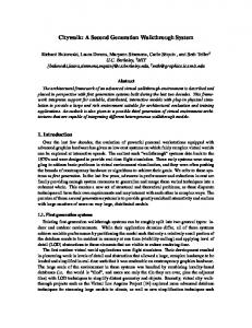
Figure 1.1: Move to drive-by-wire The shift to x-by-wire systems has increased the importance of design and development of electronic control and software in design, development and manufacturing of automotive product lines. In the last two decades, General Motors reports (Fig. 1.2), the number of electronic control unit in cars have increased by 150% and the size of software modules increased by 9900%. This increased the cost associated with electronic control and software by 200%. In the future, cost is predicted to rise. Nihon Keizai Shimbun reports that cost associated with development effort (in Japan) for automotive related software would grow from 903 million US dollars (in 2006) to 9.1 billion US dollars (in 2014).

5


Estimated Cost Number of ECUS Software Size Mechanical Electronics Software Others

1960s

1970s

1980s

1990s

76 13 02 09

200 % 150 % 9900% Mechanical Electronics Software Others

2000s

55 24 13 08

2010s

2020s

Figure 1.2: Growth of electronic control and software in automobiles

1.2

Separation of Concerns

One of the proposed approaches for embedded systems design is platform-based design [Sangiovanni-Vincentelli et al., 2004] that emphasizes separating functional specification from architecture. Functional specification (e.g. a set of functions with data dependencies) denotes what the system is supposed to do. Architecture (e.g., a set of computational resources connected through communication links) accounts for the available hardware resources. An implementation of the specification on an architecture is an allocation of the specification to the architecture, e.g. an implementation can be a mapping of the functions to computational resources and the data dependencies to communication links. An implementation can be analyzed to check whether constraints posed by the designer such as power consumption, latency, and deadlock freedom have been met or not. If the constraints are not met, then the designer can update/modify the architecture. The architecture can be modified independent of the functional specification which speeds up the exploration of different architectures and mapping. Once the implementation meets design constraints, the specification is synthesized (e.g. code is generated) for the target architecture.

6


Function definition with data dependencies

Communication and Computation Resources h1

f2

f1 f3

h3 h2

Common Semantics Domain (Platform) Application Space

System Specification

System Architecture

Architecture Space

Mapping Performance Analysis Synthesis

Figure 1.3: Platform-based design

1.3

Logical Execution Time

An effective utilization of the separation-of-concerns approach has been used in Logical Execution Time (LET) Model [Henzinger et al., 2003] for task execution where specification of a task is captured by release and termination events while the actual execution time is obtained by analyzing the task relative to an architecture. At release event, a LET task is released for execution; the task output is available only when the termination event occurs. Even if the task completes its execution before the termination event arrives, the task output is not released. The interval between the release and termination event is the LET for the task. An execution of a LET task is time-safe 7


if the task completes execution within the respective LET. The LET model makes the program execution time-deterministic (no jitter) and value-deterministic (no race conditions); this supports efficient schedulability analysis which checks whether all tasks are time-safe or not. The separation of timing from functionality also helps in architecture exploration and portability. The LET model is a meet-in-the-middle approach when compared to more traditional paradigms used to ensure timing and predictability of real-time systems [Burns and Wellings, 2001], [Edwards, 2000], [Buttazzo, 1997]. Previous attempts can be broadly classified on the basis of when the evaluation of a task is available. In one approach, task evaluations are made available as soon as the execution is complete. Priorities are used to specify (indirectly) the relative deadlines of tasks. The approach is supported by efficient code generation based on scheduling theory [Buttazzo, 1997]. However the execution time of tasks varies from one real-time platform to other and this causes race conditions (non-determinism in program variables), which in turn makes program verification and analysis extremely difficult. The other approach is based on the synchrony assumption [Halbwachs, 1993] that the underlying platform is much faster than the response time of tasks and the task may be assumed to be executing in zero time (logically). In other words, analysis of the system is performed assuming task evaluations are available as soon as they are released. The approach is mathematically very expressive and supports determinism and formal verification. However compiling synchronous languages is non trivial when it comes to tasks with non-negligible execution time and distributed computing. LET model, which allows task outputs to be available only after certain instances, trades code efficiency in favor of code predictability when compared with the first approach, which makes all outputs visible as soon as they become available. When compared with the second approach, LET model (where all logical execution times are assumed to be strictly positive) trades mathematical expressiveness in favor of computational realities. 8


1.4

Logical Reliability Model

The separation-of-concerns approach used for schedulability has been extended for reliability analysis [Chatterjee et al., 2008] thus setting the foundations for a joint schedulability/reliability analysis methodology. The main idea is the separation of application dependent (“logical”) information from platform dependent (“physical”) data. The reliability requirements (of real-time tasks) is separated from the reliability characteristics of hosts (on which the tasks execute). Reliability requirements are specified by Logical Reliability Constraint (LRC) and the architecture ensures Singular Reliability Guarantee (SRG). In the analogy between timing and reliability, LRCs play the role of release times and deadlines, while SRGs play the role of worst-case execution times. The timing analysis checks that all tasks get access to execution no less than the respective worst-case execution time (WCET); in case of transmission of output, worst-case transmission time (WCTT) should also be accounted. The reliability analysis checks that SRG for all tasks meets the respective LRC. In the reliability model, each input and output variable of a task is assigned a LRC. As tasks read and write the variables, this implicitly defines LRCs for the tasks. Each variable is associated with a LRC which is a real number between 0 and 1. LRC denotes the fraction of all periodic writes (to the variable) in the long run that are required to be valid e.g. if LRC of a variable is 0.9, then in the long run, at least 0.9 fraction of all periodic writes to this variable are required to be valid values; thus LRC is also referred as long-term reliability constraint. LRC, similar to release and termination event, is independent of the architecture. Given an architecture on which a task (writing to a variable) executes, SRG of the variable (relative to that architecture) can be computed. SRG, a real number between 0 and 1, denotes the probability with which the variable would be assigned a reliable value at an update instance. Similar to WCET/WCTT, SRG depends on the

9


underlying architecture, and is computed from the reliability of the components of the architecture. For example, consider a task executing on a host; the task periodically reads from a reliable input and writes to a variable. The host has a reliability of 0.8 i.e., the probability that the variable has a valid value at the end of task execution is 0.8; in other words SRG of the variable for the architecture is 0.8. If the task is replicated on two such hosts, the updated SRG is .96 (= 1 − .22 , i.e., the probability that at least one host is executing), assuming reliable communication and reliable inputs. If the SRG is no less than the LRC, then the implementation (of the task on the host) is reliable for the variable. SRG is a guarantee for each invocation of the task i.e., it ensures short-term reliability; thus SRG is also referred as short-term reliability guarantee. The analysis checks whether the SRG ensures the LRC or not; this is similar to schedulability analysis which checks whether the WCET/WCTT can be accommodated within the LET or not.

1.5

Refinement

Given a LET task and a host on which the task is implemented, schedulability analysis checks whether the WCET of the task (on that host) is less then the LET of the task. If there are multiple tasks, then a detailed schedulability analysis (e.g. aperiodic task scheduling) may be performed. Consider two tasks t1 and t2 executing in parallel (Fig. 1.4.a). The LET of respective tasks are denoted by the rectangles. An aperiodic EDF scheduling analysis can be performed to check whether the tasks are time-safe or not. If there is another set of tasks, t2 and t3 (Fig. 1.4.b), then the schedulability analysis need to be repeated. Consider the schedulability analysis is done for a third set of tasks a2 and a13 (Fig. 1.4.c). The LET and WCET of the tasks t2 and a2 are identical; also the release event of a13 is later than the release events of t1 and t3, termination event of a13 is earlier than the terminations events of t1 and t3, 10


and WCET of a13 is larger than both t1 and t3. Under the above conditions, if a2 and a13 are time-safe, then the other two combinations are also time-safe. Thus if schedulability analysis is performed on a2 and a13, the analysis need not be repeated for the other two sets of tasks which reduces the number of checks. The combination a2 and a13 is referred as an abstract specification and the other two combinations are concrete implementations of the abstract specification. Task t2 is a refinement of task a2; while both tasks t1 and t3 are refinement of task a13. Refinement reduces the validation effort: only abstract specification need to be analyzed and if each concrete task (in the concrete implementation) is a refinement of a task in the abstract specification, then the validation need not be repeated. In the above example, there are only two concrete specifications; in real example there can be arbitrary number of concrete specifications.

a2 a13 abstract specification t2

t2 t1

t2 t3

t2 t1

t3

concrete implementation 1 (a)

(b)

concrete implementation 2

(c)

Figure 1.4: Overview of task refinement If an abstract specification is time-safe (schedulable), then any concrete implementation that refines the abstract specification is also time-safe (schedulable). This is a sufficient condition i.e. there may be concrete implementations which are schedulable but the corresponding abstract specification may not be schedulable. The condition being sufficient denotes that resource usage is over-approximated; however refinement reduces the validation effort significantly and introduces flexibility in system design. 11


Refinement constrains the timing interface of the tasks and not the IO interface or the task functionalities. The approach can be extended for reliability analysis too. Consider a situation where task a13 reads from a reliable input and writes to a variable v13. If the reliability of the host for the period of execution of a13 is 0.9, then the SRG for v13 is 0.9. It can be shown that if the LRC of v13 is not greater than 0.9, then the implementation is reliable. Let task t1 reads from a reliable input and writes to a variable v1. If the LRC of v1 is less than the LRC of v13, then the implementation is reliable for task t1; in other words, if implementation of abstract specification is reliable, then the implementation is reliable for a concrete specification, with some restrictions on LRCs of output variables. Note the analysis (for concrete specification) is done by comparing the LRCs of the outputs of the tasks instead of comparing the SRG and the LRC of variable v1.

1.6

Hierarchical Timing Language

Hierarchical Timing Language (HTL) is a coordination language for hard real-time systems. Like it predecessor Giotto [Henzinger et al., 2003], HTL builds on the LET model of task execution. The HTL model allows sequential, parallel and conditional composition of LET tasks; and encompasses the refinement model to offer hierarchical layers of abstraction. While the layers of abstraction add structural conciseness to program specification, the refinement property reduces effort in schedulability and reliability analysis. Thus, feasible schedules for lower layers can be efficiently constructed from feasible schedules for higher layers; and if implementation is reliable for higher layers, then the implementation is reliable for lower layers. The HTL model accommodates a more general model than the LET as it extends composition and refinement from single tasks to task group with precedence. 12


While the model of task execution in HTL is LET, the tasks in HTL communicate with each other (and with the environment) through so-called communicators. A communicator defines a sequence of real-time instances of a static variable. Sensors and actuators are special cases of communicators. Task reads and writes specify communicator instances. As the read and written time instances of communicators are fixed by a program, they remain unchanged when the context of the program is modified e.g. ported to another architecture. This implies that the communicator instances (a task reads from and write to) specify the LET for the task. Each communicator is also specified a LRC. Tasks read from and write to communicators; thus LRC of the communicators implicitly specify the LRC of the task. In other words, the communicators specify both the timing and reliability requirements on tasks. Composition and refinement constraints, and program execution ensures determinism.

1.7

Overview

Chapter 2 presents an overview of the LET model of task execution, the communicator model of communication and the logical reliability model. Next the schedulability and reliability analysis is defined for a group of periodic tasks, followed by a discussion of schedulability- and reliability-preserving refinement. Chapter 3 presents an overview of HTL: the structural components (programs, modules, modes and refinement), the communication model (communicators and ports), and the task model (declaration and invocation). The formal definitions and the relation between components across levels of refinement are also presented. Chapter 4 discusses the operational semantics of HTL. The semantics is independent of the implementation (distribution of program modules) or performance guarantee of the architecture on which the program is implemented.

13


Chapter 5 presents certain structural constraints on HTL and discusses key properties on execution behavior of such constraints. The constraints ensures that there is no race in updating program variables. This makes the program execution deterministic i.e., given sufficient execution speed the values of program variables are determined by the values of the sensors. Chapter 6 discusses the schedulability analysis for an HTL implementation which is a mapping of an HTL program on an architecture. The chapter presents the execution of an implementation followed by the formal definition of schedulability analysis. Lastly, it is shown that for schedulability- preserving implementation, if the implementation of the root program without refinement is schedulable, then the whole program (root program with refinement) is schedulable. Chapter 7 discusses how to incorporate the LRC model into HTL and to perform reliability analysis. The formal definition of reliable HTL implementation is followed by reliability analysis. The chapter concludes with a discussion of how reliabilitypreserving refinement helps is avoiding repetitive reliability analysis. Chapter 8 presents an HTL compiler for a virtual machine, the Embedded Machine. An overview of the Embedded Machine is followed by the algorithms for code generation from HTL to Embedded Machine code. Chapter 9 presents HTL modeling and subsequent analysis of three controllers: a controller for three tank system, a steer-by-wire controller for automotive system, and a fly-by-wire controller for unmanned helicopter. Chapter 10 compares the work with other programming languages including timed languages (Giotto and its successors), real-time extensions of conventional languages and languages for specialized real-time applications. Chapter 11 concludes the thesis by reviewing the core concepts presented and possible future directions.

14

Chapter 2 Programming Model The computation model is based on LET model of task execution. A brief overview of LET model from previous work is presented in Section 2.1 followed by a discussion on the extension of LET models used in this work. The communication model in the framework is centered around communicators. A communicator [Ghosal et al., 2006a] is a typed variable that can be accessed (read from or written to) only at specific time instances. These time instances are periodic and specified through a communicator period. Communicators are used to exchange data between tasks. A task reads from certain instances of some communicators, computes a function, and updates certain instances of the same or other communicators. Communicators are also used to exchange data between tasks and environment. Input communicators are updated by physical sensors (possibly through drivers) and read by tasks. Output communicators are updated by tasks and read by physical actuators (possibly through drivers). Expressing LET with communicators is discussed in Section 2.3. Section 2.4 discusses the reliability model: the logical requirement and performance guarantee. Section 2.5 formally presents the reliability analysis for a set of periodic tasks. Section 2.6 extends the analyses for refinement.

15

Chapter 2. Programming Model

2.1

Logical Execution Time Model

The Logical Execution Time (LET) model of task execution separates logical timing requirements from actual physical platform execution. A LET task is sequential code with its own memory space (henceforth referred as local memory) and without internal synchronization points. The logical specification consists of a set of program variables (henceforth referred as input variables) read by the task, a set of program variables (henceforth referred as output variables) updated by the task and timing constraints. The program variables are global i.e. they can be accessed by any other task; local memory of a task cannot be accessed by any other task. Logical timing constraints are specified by a release event and a termination event; the events are triggered by clock ticks or sensors interrupts. The release and termination events determine the LET of the task; the termination time strictly follows the release time. At release event, the task reads input variables to the local memory of the task. At termination event, the task updates program variables by the result of the computation (defined by the sequential code) on the state of local memory at the release event. The copying of program variable to local memory (and vice versa) is done synchronously i.e. in logical zero time. The task may not immediately start execution at release event. The underlying platform (or the scheduling strategy) determines when the task execution should start, get preempted and resumed. Between the release and termination event, the task may be preempted and resumed any number of times. Upon completion it may give out a completion event (if required by specification) and stores the value of the computation to local memory. At the termination event, the output variables are updated from the local memory. A LET task is time-safe for a given host if the task completes execution on that host before the termination event occurs. A task, executing on a host (where no other task is executing), is time-safe if the worst-case execution time (WCET) is less than

16


release event

termination event

Logical Execution Time (LET) completion event

Logical task t running

running

Physical release

start

preemption

resume

completion

input variables read to local memory

termination

output variables written from local memory

Figure 2.1: LET model of task execution the LET duration. For multiple tasks, this entails a detailed schedulability check. If tasks are race free (i.e. at any instance at most one task writes a program variable) and a program variable is written before it is read (at any update instance), then timesafe LET tasks are time and value deterministic, portable and composable [Henzinger and Kirsch, 2002]. The output variables of a LET task are updated when the termination event occurs, even if the task completes its physical execution earlier. The input variables are read to local memory when the release event occurs, and not when the task actually starts executing. As a consequence, a LET task always exhibits the same behavior in the value and time domain on different hosts as long as the task is time-safe. Fig. 2.2 shows LET task t and two possible physical executions of the task. Consider any instant in the execution (shown by the vertical dashed line): irrespective of the execution pattern, the values of output variables remain invariant. Fig. 2.3 shows two tasks t1 and t2 with identical LETs. Task t2 reads the output of t1. For the two possible physical execution pattern shown, the value of the output variable (written by t1) will be identical because output is not updated (and thus cannot be used by task t2) until the termination event. This makes the model value-deterministic. 17


release event of t

termination event for t release event of t1 and t2

termination event for t1 and t2

Task t

Task t1 Task t2 t1

release

termination

t2

release of t1 and t2

termination of t1 and t2 t2

Figure 2.2: Time determinism

t1

Figure 2.3: Value determinism

Time-safe LET tasks are portable. Task t (Fig. 2.4) is ported to a host with half the speed than the original one without modification of the LET. Thus LET tasks can be ported to different hosts as long as they are time-safe; the bound on the scaling is determined by the host speed. The LET model also supports composition. Two LET tasks from two hosts, can be composed on a single host without modifying individual LET of the tasks (Fig. 2.5). Refer to [Matic and Henzinger, 2005] for detailed analysis of portability and composability of LET model. release event for t1 and t2

release event

termination event for t1 and t2

termination event t1

t

release of t1

termination of t1 t2

t ported to a hardware with half the efficiency release

t1

release of t2

t2

t2 termination of t2

P1 and P2 are composed on a single hardware t2 t2 t1 t2 t1

termination

release of t1 and t2

Figure 2.4: Portability

termination of t1 and t2

Figure 2.5: Composability

18


2.2

Extension of LET Model

To account for distributed implementation, the LET model is extended to include both execution and transmission of output (Fig. 2.6). In particular, along with WCET of a task, worst-case transmission time (WCTT) for the communicating network is required to decide whether the task is time-safe or not. termination event

release event Logical Execution Time (LET) Logical

completion event task t running

running

transmitting

Physical release start

completion

termination

Figure 2.6: Task execution and transmission The LET model is also extended to account for failures of the input variables. Three models are considered: • series - if one of the input variables is not reliable the task fails to execute • parallel - if any one of the input variables is not reliable, then the task may execute (possibly with an pre-assigned value for the input variable); the task fails to execute if all of the input variables are unreliable • independent - if an input variable is unreliable, the task considers a pre-assigned value for that input variable; the task may execute even if all of the input variables are unreliable. The LET model is extended to account for reliability of output program variables. A output variable may have an unreliable value if a task fails to execute and/or the 19


memory fails to store the value of the variable. The task algorithms are assumed to be correct i.e., if a task executes reliably, then the task generates the desired output for given input. The model is formally discussed in Section 2.5.

2.3

Communicators and Logical Execution Time

A task reads from certain instances of some communicators, computes a function, and updates certain instances of the same or other communicators. Fig. 2.7 shows the interaction between four communicators (c1, c2, c3, and c4 with periods 2, 3, 4 and 3 time units respectively) and three tasks (t1, t2 and t3). Task t1 reads the second instances of c1 and c4 and updates the fourth instance of c2. Task t2 reads the second instance of c3 and updates the sixth instance of c1 and the fifth instance of c2. Task t3 reads the sixth instance of c1 and updates the fifth instance of c4. The latest read and earliest write instances specify the LET for the tasks: the latest read instance determines the release time, and the earliest write instance determines the termination time. The task can read any communicators before the latest read time but cannot be released; similarly it must complete execution before the earliest communicator instance it writes to. Task t1 reads c1 at time 2 and stores the value in local memory; the task cannot be released at time 2 as it has not read all the inputs it needs to read. At time 3, the task reads c4; as all inputs have been read, the task is released for execution. Task t2 writes c1 and c2; as the update of c1 is earlier the task must complete execution by time 10. Thus LET of t1 spans from time 3 to time 9, the LET of t2 from time 4 to time 10, and the LET of t3 spans from time 10 to time 12. Note that the time unit is logical and has no physical significance. Only at implementation the time unit is bound to a clock, e.g, millisecond or second. For schedulability analysis, the communicator periods and execution time for tasks are assumed to be bound to the same clock. 20


reads c1

updates c4 task t3

reads c3

updates c1

updates c2

task t2 reads c1 reads c4

updates c2 task t1

c4

c4

c3

c3

c2 c1 1

2

c2 c1

3

4

c4 c3

c3

c2

c1 0

c4

c4

c2

c1 5

6

c1 7

8

c2 c1

9

10

c1 11

12

Figure 2.7: Communicators and tasks Communicators communicate between the environment and tasks (Fig. 2.8). The input communicators can only be written by the environment; i.e., values of input communicators are input from the environment. Typically an input communicator is updated by a physical sensor, possibly through drivers and read by a task. The output communicators can only be read by the environment, i.e., values of output communicators are output to the environment. Typically a task updates an output communicator, and a physical actuator reads the output communicator, possibly through a driver. Any other communicators can both be read and written by tasks. Tasks define the input/output interface through communicators and thus communicators are the key to compose tasks. Task composition is deterministic i.e. given sufficient CPU speed for time-safety, the real-time behavior of the LET tasks is determined by the input (i.e., the values of all sensor communicator instances), independent of the host speed and utilization. The determinism in task composition is ensured in two ways. First, update races on communicators are prohibited i.e. different tasks 21


sensor writes input communicator s (possibly though drivers)

t writes c

task t

s t' read s

task t

c task t'

t' read c

t writes a a

task t'

actuator reads output communicator a (possibly though drivers)

Figure 2.8: Communication via communicators cannot write to the same instance of a communicator. Second, if a communicator update is due at any instance then the communicator is updated before it is read. The first is ensured by structural properties (e.g.

task input and output) and the

second is ensured by execution properties.

2.4

Logical Reliability Model

A communicator may have an unreliable value if a task fails to execute and/or the memory fails to store the value of the communicator. An application accessing the communicator must specify the tolerance of the unreliable values for the communicator: the tolerance is specified through Logical (long-term) Reliability Constraint (LRC). Each communicator has a specified LRC, where the LRC denotes the desired fraction of reliable values of the communicator that the system expects in the longrun. For example, if LRC for a communicator c is 0.9, then .9 fraction of all instances of communicator c on all execution (in the long-run) should have reliable values. Fig. 2.9 shows a sample execution trace with the value of communicator c at the first twenty instances. The communicator has type integer; an unreliable value is denoted by ⊥. For the given trace, there are 20 instances of communicator c out of which 18 are reliable i.e. the fraction of reliable values is 18/20 = .9. If an implementation used the communicator c, then the above fraction must be .9 for all execution traces 22


in the long-run. It is assumed if a task fails to execute or memory fails to hold value, a ⊥ would be generated; i.e. any integer value (in the last example) is reliable.

c

c

T

4

2

3

1

5

4

6

4

8

4

3

4

c

c

c

c

c

c

c

c

c

c

c

c

1 + 1 + 0 + 1 + 1 + 1 + 1 + 1 + 1 + 1 + 1 + 1 + 1+

T

2

3

4

c

c

c

6 c

4 c

8 c

1 + 0 + 1 + 1 + 1 + 1 + 1 = 18/20 = 0.9

Figure 2.9: Fraction of reliable values Similar to LRC, each communicator is associated with an Singular (short-term) Reliability Guarantee SRG, a fraction between 0 and 1. SRG=0.95 means the probability that a host fails during the execution of a task (writing to the communicator) is 0.05; i.e., given reliable inputs to a task executing on the host, the probability that the task writes ⊥ to the communicator is 0.05. Fig. 2.10 shows a task t which reads from an input communicator s (with LRC=1) and writes to an output communicator a (with LRC=0.9) periodically. LRC=1 suggests that the sensor is 100% reliable. The task can only fail if the host on which it is implemented fails to execute. The task algorithm is assumed to be correct. Consider the task is implemented on a host h with reliability .95. There being no replication the SRG is also equal to .95. In other words for every iteration of task t, the probability that there is reliable output at a is at least 0.95. In this case, the LRC is satisfied by the SRG as SRG is greater than LRC; Section 2.5 presents the formal reasoning. In a different scenario if a host h0 with reliability 0.8 is considered then the LRC is not satisfied (LRC > SRG). However if two replications of h0 are available, then task t can be replicated on both the hosts. The new SRG = 1 − (1 − .8)2 = .96 (probability that at least one host is reliable) which is greater than the required LRC. The SRG is computed by reaction block diagram (RBD) modeling. Refer Appendix A for details on RBDs. The hosts are assumed to be connected over a reliable broadcast network. Section 2.5 present the analysis for multiple inputs and different input failure models. 23


specification

architecture 1

architecture 2

host h' s

task t

LRC = 1

a

host h

LRC = 0.9

reliability=0.95

reliability=0.8

SRG=.96

host h'

SRG = 0.95

Figure 2.10: Intro to reliability analysis Reliability analysis on the logical reliability model can be preserved over refinement. Fig. 2.11 shows two tasks t and t0 where t0 refines t. Both the tasks read from identical input and execute on same host. Task t writes to actuator a, while task t0 writes to actuator a0 . Let the host be reliable for t i.e. the SRG is no less than the LRC of a. If the LRC of a0 is no more than the LRC of a, then host is also reliable for t0 ; the SRG cannot be less than the LRC of a0 from mathematical comparison. Instead of repeating the reliability analysis, comparison of the LRCs of the outputs of the tasks concluded the reliability of the host to task t0 .

s s

task t task t'

LRC(a') ≤ LRC(a)

a a'

If LRC(a) is satisfied, then LRC(a') will be satisfied

Figure 2.11: Reliability preserving refinement As discussed in Chapter 1, LRC and SRG is an approach to reliability analysis, as LET and WCET is an approach for timing analysis. The idea is based on separating requirements from guarantees. Timing requirements are expressed through release and termination events while performance guarantee (for an architecture) is expressed through WCETs. Release and termination events are application dependent “logical” information while WCETs are architecture dependent “physical” data. Similarly, 24


LRC is application dependent “logical” information for desired reliability, while SRG is architecture dependent physical data on reliability that can be guaranteed. Timing analysis checks whether the “physical” data ensures the “logical” requirement for timing i.e. whether the LET is enough to ensure allocation for WCET time units. Similarly reliability analysis checks whether the “physical” data ensures the “logical” requirement for reliability i.e. whether the SRG is enough to ensure the LRC.

2.5

Reliability Analysis

The section presents the reliability analysis (based on the logical reliability model) for a set of periodic tasks running on a set of hosts connected over a broadcast network.

System A system (S, A, I) consists of specification S, architecture A and implementation I. A specification S = (tset, cset) consists of a set of tasks tset and a set of communicators cset, where tasks and communicators are declared as follows. A communicator declaration (c, type, init, π, µ) consists of a communicator name c, data type type, an initial value init, an accessibility period π ∈ N>0 and LRC µ ∈ R(0,1] . All communicator names are unique i.e. if (c, ·, ·, ·, ·) and (c0 , ·, ·, ·, ·) are two distinct communicator declarations then c 6= c0 . Given a communicator c ∈ cnames(P), the type type[c] denotes the range of values the communicator can evaluate to and init[c] ∈ type[c] denotes the initial value of the communicator. The data type includes a special symbol ⊥ to indicate unreliable communicator value; a non-⊥ value indicates that the communicator has a reliable value. The evaluation of a communicator val[c] is a function that maps c to a value in type[c]. The period and LRC of a communicator c is denoted as π[c] and µ[c] respectively.

25


A task declaration (t, ins, outs, fn, fmodel, default) consists of a task name t, a list of inputs ins, a list of outputs outs, a function fn, an input failure model fmodel ∈ {1, 2, 3} and a list of default values default. All task names are unique i.e. if (t, ·, ·, ·, ·, ·) and (t0 , ·, ·, ·, ·, ·) are two distinct task declarations then t 6= t0 . Given a task t, the inputs, outputs, function, fault model and default values are denoted as ins[t], outs[t], fn[t], fmodel[t] and default[t] respectively. An element of the input/output list is a pair (c, i) consisting of a communicator name c ∈ cset and a communicator instance number i ∈ N≥0 . The j-th element of the input list is denoted as insj [t] where 1 ≤ j ≤ |ins[t]|. The k-th element of the input list is denoted as outsk [t] where 1 ≤ k ≤ |outs[t]|. For a task t, the length of input list is |ins[t]| and the length of output list is |outs[t]|. If insj [t] = (c, ·), then type(insj [t]) = type[c]; similarly if outsk [t] = (c0 , ·), then type(outsk [t]) = type[c0 ]. If |ins[t]| = m and |outs[t]| = n, then the function fn[t] is, fn[t] : Π1≤j≤m type(insj [t]) → Π1≤k≤n type(outsk [t]). Let rcset[t] be the set of communicators read by task t. The input failure model fmodel[t] denotes the action of a task if one or more inputs are unreliable; the list default[t] is a list of default values for the communicators in rcset[t]. The three failure models are: • series (fmodel[t] = 1): if any one of the inputs fails, the task fails to execute • parallel (fmodel[t] = 2) if an input is unreliable, the task may execute by using the default value of the communicator from the list default[t]. If all of the inputs are unreliable the task fails to execute. • independent (fmodel[t] = 3) if an input is unreliable, the task uses the corresponding default value for that input from the list default[t]. The task may execute even if all inputs are unreliable.

26


For a task t, read time rtime[t] is the latest communicator instance t reads from and write time ttime[t] is the earliest communicator instance t writes to. Formally, rtime[t] = maxj (π[c] · i) where insj [t] = (c, i) and ttime[t] = mink (π[c0 ] · i) where outsk [t] = (c0 , i). The tasks repeat with periodicity π[S] where π[S] = lcm(cset) · d(maxt∈tset ttime[t])/(lcm(cset)e and lcm(cset) is the least common multiple of the communicator periods. The restrictions on task declarations are as follows: (1) all tasks read from some communicators and write to some communicators, (2) for all tasks, read time is strictly earlier than the write time, (3) no two tasks write to the same communicator, and, (4) no task can write a communicator instance multiple times. In other words, a communicator can be written by at most one task at any instance, i.e., the specification is race free. An architecture A is a tuple (hset, sset, C[S]) where hset is a set of hosts (connected over a reliable broadcast network), sset is a set of sensors and C[S] is a set of architectural constraints for a given specification S = (tset, ·). The constraints are: (1) reliability of hosts and sensors specified by host reliability map hrel : hset → R(0,1] , and sensor reliability map srel : sset → R(0,1] ; and, (2) execution metrics for the tasks specified by worst-case-execution-time (WCET) map, wemap : tset × hset → N>0 and worst-case-transmission-time (WCTT) map, wtmap : tset × hset → N>0 . The hosts are assumed to be fail-silent [Cristian, 1991] i.e. if a host fails, then it does not produce any garbage output. In other words, a host works correctly or stops functioning (becomes silent). If tasks are replicated on several fail silent hosts, then all faulty components do not produce any output while all working components produce identical output for a given cycle of computation. In [Baleani et al., 2003], the authors argue that fail-silence can be achieved at reasonable cost. To keep the analysis simple, the broadcast network is assumed to be reliable. Non-reliability in broadcast network can be accounted in the model as long as the faulty behavior is 27


atomic i.e. if the broadcast fails then none of the hosts receives any input. The WCTT is measured as the broadcast time for each task from each host. Memory is assumed to be 100% reliable. Given a specification S = (tset, ·) and an architecture (hset, ·, ·), an implementation I is a function from tasks to a set of hosts i.e. I : tset → 2hset \ ∅. The implementation is assumed to distributed i.e. there are multiple hosts and all tasks are not implemented on a single host. Tasks can also be replicated on multiple hosts. If a task t is mapped to multiple hosts then each host h executes a local copy of t; the local copy is referred as a task replication (t, h). All communicators c are replicated on all hosts h; each local copy of communicator is referred as a communicator replication (c, h). When a task replication completes execution, it broadcasts the output to all hosts (to update relevant communicator replications).

Semantics An execution of an implementation, also called an implementation trace (or simply trace), is a (possibly infinite) sequence of communicator values for every time instance. A time instance (or simply an instance) is a sequence of positive integers and denotes the harmonic fraction of all communicator periods. In practice, time instances are generated by the architecture through clock interrupts. We will assume the following. (1) Time instances are global i.e. synchronized across all hosts. (2) If a sensor s is replicated over multiple hosts, then the environment writes identical values to all replications of s when the update is due. (3) At any instance, if a communicator c is updated, then all replications of c are first updated and then read. The above constraint and exclusion of races ensure that all communicator replications have unique values when they are read. (4) When a task replication (t, h) completes execution, it broadcasts the output (to be written to a communicator c)

28


to all hosts hset/{h}. Every host receives the values from each replication of t and stores them in a local memory space (assigned to c). When update of c is due, voting is used to decide on the final value to be written to the communicator replication on the host. All tasks are functionally correct and given identical inputs provide identical outputs. All replications of a task have identical input failure models. At any given iteration, the replications of a task either generate ⊥ (unreliable execution) or the correct value. Thus if some replications generated a non-⊥ value then all other replications which executed reliably generated the identical non-⊥ value. This makes the voting straightforward. If there is at least one non-⊥ value, the communicator replication is assigned that value. The semantics is formally defined as follows. For i ≥ 0, let Xi be a function from the communicator set to the set of values, with possibly the empty set i.e., Xi : cset → typehset ∪∅, where type = ∪c∈cset type[c]. If i mod πc = 0, then Xi (c) ∈ typec hset , otherwise ∅. A trace is an infinite sequence (Xi )i≥0 of such functions. The semantics is the set of all possible traces.

Reliability , the value of α is reliable if α contains at Given a communicator c, and set α ∈ typehset c least one non-⊥ value. A reliability based abstraction consists of only values 0 and 1, where 1 denotes reliable value, and 0 denotes unreliable value. Given a trace (Xi )i≥0 , we define the reliability based abstraction trace (Zj )j≥0 = ρ((Xi )i≥0 ) as follows, Zj : cset → {0, 1}; Zj (c) = 1 if the set Xj·πc (c) is reliable, 0 otherwise. In other words, the function ρ maps a trace (Xi )i≥0 to another trace (Zj )j≥0 ; the second trace is referred as reliability-based abstract trace. We define the limit average value of a reliability-based abstract trace for communicator c, τ c = (Zj (c))j≥0 as the “long-run” average of the number of 1’s in the abstract trace. Formally, the limit-average value

29


limavg(τc ) of a reliability-based abstract trace for communicator c, τc = (Zi (c))i≥0 is n−1 1X defined as: limavg(τc ) = lim Zi (c). Given a communicator c, the set of reliable n→∞ n i=0 abstract traces, denoted as traces c , is the set of reliability-based abstract traces for c with limit-average no less than µ[c] i.e. traces c = {τc : limavg(τc ) ≥ µ[c]}. Given set of communicators cset = {c1 , c2 , · · · , ck }, the set of reliable abstract traces is traces cset = {(Zj (ci ))j≥0 : ∀1 ≤ i ≤ k.limavg((Zj (ci ))j≥0 ) ≥ µ[ci ]}.

Analyses on Implementation Given an implementation I for a specification S on an architecture A, we define the following analyses: • Schedulability analysis. The implementation I is schedulable if (all replications of) all tasks complete execution and transmission (of the outputs) between the read and the write time of the respective task [Ghosal et al., 2006a]. • Reliability analysis. The implementation I is reliable if for each communicator, long-run average of the number of reliable values observed at access points of the communicator is at least LRC of the communicator. An implementation I is valid for a specification S on an architecture A, if I is schedulable and reliable.

Reliability Analysis A specification graph GS = (VS , ES ) with ES ⊆ VS × VS is defined as follows. The set of vertices is VS = {(c, i) : c ∈ cset ∧ i ∈ {0, · · · , π[S]/π[c]}} ∪ {t : t ∈ tset}. The set of edges is ES = {((c, i), t) : (c, i) ∈ ins[t]} ∪ {(t, (c, i)) : (c, i) ∈ outs[t]} ∪ {((c, i), (c, i0 )) : i < i0 ∧ ∀t ∈ tset.∀i < i00 ≤ i0 .(c, i00 ) 6∈ outs[t]} ∪ 30

Chapter 2. Programming Model {((c, π[S]/π[c]), (c, 0))|c ∈ csetnino }. The set csetnino ⊆ cset is the set of all noninput non-output communicators. A communicator cycle is a path δ from (c, i) to (c, i0 ) such that the path δ contains at least one vertex t ∈ tset. A specification S is memory free if the specification graph GS contains no communicator cycle. Given the constraints on tasks and assumptions on architecture, environment and semantics, the task replications can be assumed to be connected in parallel to each other. Each block of such task replications are connected in series with parallel blocks of replications of other tasks. Given an implementation I, reliability of a task Q t, λt = 1 − h∈I(t) (1 − hrel(h)), i.e., at every iteration the probability that the task t executes is at least λt . SRG λc of a communicator c is inductively defined as follows: (a) for an input communicator c we have λc = srel(s) where c is updated by sensor s; (b) for an non-input communicator c let t be the task that writes c and let SRGs of the communicators in the set icsett be defined, then λc is defined as follows: (1) if Q fmodel[t] = 1, then λc = λt · c0 ∈rcset[t] λc0 , (2) if fmodel[t] = 2, then λc = λt · (1 − Q c0 ∈rcset[t] (1 − λc0 )), and (3) if fmodel[t] = 3, then λc = λt . With the constraints on task declarations, a non-input communicator c can be written by a single task. Given an implementation I, at every iteration the probability that a non-input communicator c has a reliable value is at least λc . The input communicators are written at every step by the environment. For an implementation I, at every iteration the probability that input communicator c has a reliable value is at least λc . Hence from the definition of local (or one-step) probabilities we obtain a probability space Pr I (·) on the set of infinite traces. Definition 1. Given a memory-free specification an implementation I is reliable if the probability of the set of reliable abstract traces is 1, i.e., Pr I [traces cset ] = 1. Next a reliability analysis is proposed; the analysis compares the LRCs and SRGs

31


for all communicators and decides on the reliability of the implementation from the comparison. For proof of the proposition, the Strong Law of Large Numbers (SLLN) [Durrett, 1995] is used; SLLN states that: Let X1 , X2 , · · · be independent and identically distributed with E|Xi | < ∞. Let EXi = µ and Sn = X1 + X2 + · · · + Xn . Then Sn /n → µ almost surely as n → ∞. Proposition 1. Given a memory-free, race-free specification, an implementation is reliable if for all communicators c, we have λc ≥ µ[c]. Proof. Let Yi (c) be a random variable denoting the reliable value for c at instance i·π[c]. Since the specification is memory-free, it follows that the sequence (Yi (c))i≥0 is independent, and from the constant reliability of the hosts we obtain that the random variables are also identical. Let E[Yi (c)] = β, and by SRG of c, we have β ≥ λc . Let P Sn Sn = n−1 i=0 Yi . Applying the strong law of large numbers (SLLN), we obtain that n converges almost-surely to β. Formally, we have the following, ∀ > 0.

Pr I ({τ : | Snn(τc ) − β| > infinitely many n’s}) = 0

∀ > 0. Pr I ({τ : | Snn(τc ) − β| < ultimately forall n’s}) = 1 ∀ > 0.

Pr I ({τ : | limn→∞

Sn (τc ) n

Pr I ({τ : limn→∞

− β| < }) = 1

Sn (τc ) n

= β}) = 1.

Since β ≥ λc , the desired result follows. If the specification graph has a cycle then the result does not hold for all task models. Consider a task t, with fmodel[t] = 1, that reads and writes to a communicator c. Once ⊥ is written, then the value of c is always ⊥ from that instance. Hence if λ[t] < 1, then the long-run average of the number of reliable value of c is 0 with probability 1. The source of the problem is that the value of the communicator at any iteration is dependent on the value of the communicator in the previous 32


iteration. In other words, the values of communicators are not independent contrary to the assumption made in the proof. The solution to the problem is that for each communicator cycle, there should exists at least one task in the cycle with input failure model ‘independent’. The failure model ensures that even if there is a faulty input, the output is independent of the failure as a default value would be used. This ensures that for every communicator the random variable values at different iterations is independent

Time-Dependent Implementation Consider two tasks t1 and t2 that write to two communicators c1 and c2 , respectively. The LRCs of both the communicators is 0.9. Let h1 and h2 be two hosts with reliability 0.92 and 0.88, respectively. An implementation that maps t2 to h2 violates the reliability requirement for c2 , and an implementation that maps t1 to h2 violates the reliability requirement for c1 . The above implementation is time-independent i.e., the tasks are always executed on same host. A time-dependent implementation is one where tasks are executed on different sets of hosts depending on the time of their execution. For example, a time-dependent implementation may map the tasks t1 and t2 alternately to hosts h1 and h2 . This implementation is reliable. Our definition of reliability for implementation is general enough to allow such time-dependent implementations.

2.6

Refinement

A specification can be replaced by another specification; the first one is referred as refined specification and the second one as refining specification. Every task in the refining specification maps to a unique task in the refined specification such that no

33


two tasks in the refining specification can map to the same task in the refined specification. We will show that if an implementation is valid for a refined specification and all tasks write to communicators whose LRC do not exceed the LRC of communicators being written by the task (in refined specification) it maps to, then the implementation is valid for the refining specification. Consider two systems (S, A, I) and (S0 , A0 , I0 ), where S = (tset, cset), S0 = (tset0 , cset0 ), A = (hset, sset, CS ), and A0 = (hset0 , sset0 , CS0 ). Let κ be a total and one-to-one function from tset0 to tset. The system (S0 , A0 , I0 ) refines system (S, A, I) under κ, denoted as (S0 , A0 , I0 ) ≤κ (S, A, I), if the following set of refinement constraints are met: (a) hset = hset0 , (b) for all tasks t0 ∈ tset0 , we require 1. I(t0 ) = I(κ(t0 )), i.e. tasks t and t0 are mapped to the same set of hosts 2. ∀h ∈ I(t0 ) : wemap(t0 , h) ≤ wemap(κ(t0 ), h) and wtmap(t0 , h) ≤ wtmap(κ(t0 ), h), i.e. tasks t and tasks 0 have identical WCET and WCTT for any host 3. rtime[t0 ] ≤ rtime[κ(t0 )] and ttime[t0 ] ≥ ttime[κ(t0 )], i.e. latest read time of t0 is not later than that of t and earliest write time of t0 is not earlier than that of t 4. if (c0 , ·) ∈ outs[t0 ], then µ[c0 ] ≤ max(c,·)∈outs[κ(t0 )] µ[c], i.e. the LRC of any communicator written by task t0 should be less than the maximum of the LRCs of the communicators written by task t 5. fmodel[t0 ] = fmodel[κ(t0 )], i.e. fault model of the tasks t and t0 are identical, and, 6. if fmodel[t0 ] = 1, then rcset[t0 ] ⊆ rcset[κ(t0 )], i.e. if task t0 has input failure model 1, then the set of communicators read should be a subset of the communicators read by task t, and, 34

Chapter 2. Programming Model 7. if fmodel[t0 ] = 2, then rcset[t0 ] ⊇ rcset[κ(t0 )], i.e. if task t0 has input failure model 2, the the set of communicators read should be a superset of the communicators read by task t. Note that all the constraints are local checks on t0 and κ(t0 ). Refinement relation is reflexive, anti-symmetric and transitive. Given (S0 , A0 , I0 ) ≤κ (S, A, I), we have the following result. Proposition 2. Given (S0 , A0 , I0 ) ≤κ (S, A, I) and I is valid for S on A, then I0 is valid for S0 on A0 . Proof. The result follows from Lemmas 1 and 2. Lemma 1. If I is schedulable for S, then I0 is schedulable for S0 . Proof. Given the schedule of tset for each period, tasks in tset0 can be scheduled, for each period, in the same time slots in which the respective parent task is scheduled.

Lemma 2. If I is reliable for S, then I0 is reliable for S0 . Proof. The result follows from the fact that given a random variable X, if Pr (X ≥ µ) = 1, then for all µ0 ≤ µ we have Pr (X ≥ µ0 ) = 1.

35

Chapter 3 Hierarchical Timing Language Hierarchical Timing Language (HTL) is a coordination language. HTL can express I/O interfaces of tasks, interaction between tasks (and possibly environment), and real-time behavior of tasks; however individual tasks are implemented in foreign languages. The computation model of HTL is based on LET model of task execution. The communication model of HTL is centered on communicators. Based on the LET model and communicators, HTL provides a framework to specify (sequential, conditional and parallel) composition of tasks and refinement of task into task groups with precedence. Task composition exhibits deterministic behavior i.e. absence of races (on communicators) and consistency of value (of a communicator) at any instance. The determinism is ensured by constraints (Chapter 5) on program structure and program execution. Task refinement preserves schedulability (resp. reliability) analysis i.e. if a higher level program is schedulable (resp. reliable), then so is a lower level program provided the lower level program is a valid refinement of the higher level program. Chapter 6 discusses valid schedulability-preserving refinement and Chapter 7 discusses valid reliability-preserving refinement.

36

Chapter 3. Hierarchical Timing Language

3.1

Overview of HTL

The key structural components of HTL are: mode, module, program and refinement.

Mode In the communicator model of communication, all tasks must communicate via communicators. HTL modifies the communication model, by allowing communication between certain tasks through ports. A port is a typed variable, but unlike a communicator, it is not bound to time instances i.e., as soon as a task writes to a port, another task can read the port. Interaction through communicators may introduce latency but interaction through ports does not have any latency. Communication through communicators is referred as indirect communication, while communication through ports is referred as direct communication. HTL allows direct communication between tasks if they are grouped in a so called mode. A mode is a group of tasks with identical period of invocation and the tasks can communicate with each other through direct or indirect communication. The period of invocation is specified through a mode period. While tasks in a mode can communicate through ports or communicators, tasks in different modes must communicate through communicators only. The direct communication flow between tasks within a mode determines an acyclic precedence relation on the tasks in the mode. Fig. 3.1 shows three tasks t1, t2, and t3 in a mode m1. Task t1 reads the second instances of communicators c1 and c4, and updates a port p and third instance of communicator c3. Task t2 reads the third instance of c3 and updates the seventh instance of c1. Task t3 reads the port p and updates the fifth instance of communicator c2. The communication between t1 and t3 occurs through port p. The port p is not bound to time instances i.e., as soon as t1 completes execution, port p is 37


reads c3

mode m1

task t2 reads c1 reads c4

updates c1

updates c3 task t1 p task t3

updates c2 c4

c4

c3

c3

c2 c1

1

2

c2 c1

3

4

c4 c3

c3

c2

c1

0

c4

c4

c2

c1

5

c1

6

7

8

c2 c1

9

10

c1

11

12

Figure 3.1: An HTL mode updated. Tasks t3 can read the port p as soon as it is updated and starts execution. This essentially reduces latency to zero. On the contrary, communication via communicators may introduce latency. Task t1 and t2 communicates via communicator c3. Task t2 has to wait till time 8, when c3 is updated; t2 cannot read the evaluation even if task t1 completes execution earlier. The dependence on ports denotes a precedence relation between tasks. In mode m1, tasks t1 precedes t3. Tasks within a mode interact through ports and communicators; tasks from different modes interact only through communicators. Fig. 3.2 shows two modes m1 and m2 with periods 6 and 12, respectively. The arrows between tasks denote precedence through port access.

38


t4

mode m2

t8

t5 t7

t9

t6

mode m1

mode m1

t2

t1

t2

t1 t3

c3

c3

c2 c1 1

2

c2 c1

3

4

c3

c3

c2

c1 0

t3

c2

c1 5

6

c1 7

8

c2 c1

9

10

c1 11

12

Figure 3.2: Two HTL modes

Module In real-time applications, a group of tasks may have to be replaced by an alternate group depending on some specific condition (e.g., a certain sensor reading). HTL accommodates this by allowing mode switches at the end of mode periods, which are triggered by conditions on communicator and port values. A network of modes and mode switches is called a module (Fig. 3.3). One mode in each module is specified as the start mode; the start mode is the first to execute. In Fig. 3.3, module mdl1 has three modes m11, m12 and m13, switching between themselves. The switching between modes is denoted by the arrow between the modes; the direction of the arrow implies the switching. The start mode is m11 (denoted by an incoming arrow without source mode). A module is essentially a conditional and sequential composition of modes; conditional composition is specified by mode switching and sequential composition is ensured by the semantics that at most one mode from a module can be active at any

39


instance. Determinism in mode switching is ensured by specifying a start mode and having deterministic mode switches i.e., at any instance at most one switch of a mode

mode m22 mode m21

mode m31

mode m31

program P

mode m13

mode m21

module mdl3

mode m12

module mdl2

mode m11

module mdl1

can evaluate to true.

Figure 3.3: An HTL program with three modules

Program An HTL program is a set of modules. A program is a parallel composition of modules i.e., all modules are active at any instance. While the modes within a module are composed sequentially (i.e., at any time, the tasks of at most one mode of a module are active), the modes from different modules are composed in parallel and may interact through communicators. Communicators are used to exchange data between tasks from different parallel modules, as well as to exchange data from one task within a module to a later task within the same module (but possibly in a different mode). Fig. 3.3 shows a program P with three modules mdl1, mdl2 and mdl3.

Refinement HTL allows replacing a mode by another HTL program (Fig. 3.4); the technique is referred as mode refinement. In essence, the technique extends the refinement of task

40


concept (Chapter 2) for a group of tasks with precedence. Fig. 3.4 shows a program P with multiple levels of refinement. Program P is referred as root program; modules in root program are root modules. In the root program, modes m13, m22 and m23 are refined by programs P4, P1 and P2 respectively. In turn, mode m83 (in program P4) is refined by program P5, and mode m42 (in program P1) is refined by program P3.

mode m52

m62

mode m63

mode m72

P P2

mdl2

mode m71

P3

m61

mode m51

mdl5

mdl3

mode m42

P1

mdl9

mode m41

mode m23

mdl7

mode m02

mdl0

mode m01

mode m92

P5

mode m83

mode m91

mode m22

mdl4

m82

mdl8

m81

mode m32

P4

mode m13

mode m21

mode m31

mdl6

m12

mdl1

m11

Figure 3.4: An HTL program Refinement does not add expressiveness to the programming model. An HTL program with multiple levels of refinement can be translated into an equivalent flat program without refinement. Appendix B presents an overview of the techniques to flatten an HTL program. Even though, refinement does not add expressiveness, the techniques has two key advantages:

41


• Refinement allows structured and concise specification. Specifying all behaviors through mode switching is cumbersome, e.g. if module mdl2 (Fig. 3.4) is flattened, then it will have 10 modes and 32 mode switches. This is not only cumbersome to conceive and express, but also error-prone. • Refinement simplifies program analysis. Refinement is constrained in such a way that if an analysis holds for the root program, then the analysis holds for the whole program. Consider a program with only module mdl2. From refinement constraints, if the module is schedulable, then schedulability of the refinement of the module need not be checked. This reduces the schedulability check from 10 modes to 3 modes. The refinement constraints are informally explained through an example (Fig. 3.5). A program P has a single module mdl with single mode m. Mode m0 is refined by a program P0 with a single module mdl0 which has a single mode m0 . HTL imposes the following restrictions on m0 . First, the period of mode m0 is identical to that of m. This ensures that when m switches (which is only possible at the end of its period), then all tasks in the modes refining m have terminated execution. The constraints avoids unsafe termination of task invocations in mode m0 . Second, every task in m0 refines an unique task in m (mapping denoted with vertical arrows); e.g., t50 refines t5. HTL considers t5 as a placeholder (an abstract task) for t50 (the concrete task): the abstract task t5 does not execute at run-time but ensures that t50 is accounted for during the schedulability analysis of the root program. Therefore, (1) the latest (resp. earliest) communicator read (resp. write) of t50 must be equal to or earlier (resp. later) than that of t5; (2) every task that precedes t50 must refine a task that precedes t5; and (3) the WCET of t50 must be less than or equal to the WCET of t5. These three constraints ensure that if t5 can be scheduled in the root program, then t50 can be scheduled in the refined program. 42

t5

mode m t9

t4'

mode m' t7'

t5'

c3

c3

c2 c1 1

2

c2 c1

3

4

c3

c3

c2

c1 0

t9'

c2

c1 5

c1

6

7

8

P

t7

P'

t8

t6

mdl

t4

mdl'


c2 c1

9

10

c1 11

12

Figure 3.5: Refinement in HTL Refinement constrains the timing behavior of a concrete task (relative to the abstract task it maps to) and not the functional behavior or I/O interface. This allows expressing choice and change in task functionality. Choice is expressed when an abstract task in a mode is the parent of multiple concrete tasks (in different modes of the refinement program), each representing different execution scenario. Change is expressed when a concrete task, refining an abstract task, reads from and writes to different communicators than the abstract task. Refinement allows adding and replacing parts of program without overloading analyses. A program may contain abstract tasks which are not refined. Refinements may be added later without repeating the schedulability analysis and/or modifying the timing interfaces of other tasks. Similarly, a refinement can be replaced by another refinement without change in analyses. For example, refinement to mode m52 can be added, or program P5 can be replaced by another program without repeating schedulability analysis.

43


Distribution Many embedded applications are distributed: the tasks are distributed on several hosts and interact with each other through communication channels. In HTL, distribution is specified through a mapping of root modules to hosts. The distribution is implemented by replicating shared communicators on all hosts, and then have the tasks that write to shared communicators broadcast the outputs. The semantics (i.e., the real-time behavior) of an HTL program is independent of the number of hosts and replication, but code generation and program analyses take the distribution into account. If a root module is mapped to host h, then all the programs in the refinement of the module is mapped to host h. This is a refinement constraint under a distributed implementation. Intuitively if a root module is schedulable for a host h, the schedulability of the refinement of the root modules can be predicted (without repeating analysis) only if the refinement are implemented on the same host h. If modules mdl1, mdl2 and mdl3 (Fig. 3.4) are mapped to hosts h1, h2 and h3 respectively, then programs P4, P5 are executed on h1, and programs P1, P2, P3 are executed on host h2.

3.2

Abstract Syntax

The main components of HTL are presented in an abstract way. In practice a concrete syntax can be written from this abstract syntax (refer [Ghosal et al., 2006b]). An HTL program P is a pair (communicators, modules) where communicators is a set of communicator declarations and modules is a set of module declarations. Given a program P, the communicator and module declarations are denoted as communicators(P) and modules(P) respectively.

44


Communicator Declaration A communicator declaration (c, type, init, π) consists of a communicator name c, a structured data type type, an initial value init (if different from the default value of type), and a period of access π ∈ N>0 .

Data type indicates integer,

float and boolean. More complex data types like arrays can be defined; however types are not an integral part of the program definition and refinement properties. Hence complex type definitions has been left out. All communicator names are unique; i.e., if (c, ·, ·, ·) and (c0 , ·, ·, ·) are two distinct communicator declarations, then c 6= c0 . The set of declared communicator names for a program P is cnames(P); formally, cnames(P) = {c|(c, ·, ·, ·) ∈ communicators(P)}. Given a communicator c ∈ cnames(P), the type type(c) denotes the range of values the communicator can evaluate to and init(c) ∈ type(c) denotes the initial value of the communicator. The evaluation of a communicator val(c) is a function that maps c to a value in type(c). The period of a communicator c is denoted as π(c).

Module Declaration A module declaration (mdl, ports, tasks, modes, start) consists of a module name mdl, a set of port declarations ports, a set of task declarations tasks, a set of mode declarations modes, and a mode name start. All module names are unique; i.e., if (mdl, ·, ·, ·, ·) and (mdl0 , ·, ·, ·, ·) are two distinct module declarations, then mdl 6= mdl0 . The set of declared module names for a program P is mdlnames(P); formally, mdlnames(P) = {mdl|(mdl, ·, ·, ·, ·) ∈ modules(P)}. Given a module mdl, the port declarations, task declarations, mode declarations, and start mode are denoted as ports(mdl), tasks(mdl), modes(mdl) and start(mdl) respectively.

45


Port Declaration A port declaration (p, type, init) consists of a port name p, a structured data type type, and an initial value init (if different from the default value of type). All port names are unique; i.e., if (p, ·, ·) and (p0 , ·, ·) are two distinct port declarations, then p 6= p0 . The set of declared port names for a module mdl is pnames(mdl); formally, pnames(mdl) = {p|(p, ·, ·) ∈ ports(mdl)}. Given a port p ∈ pnames(mdl), the type type(p) denotes the range of values the port can evaluate to and init(p) ∈ type(p) denotes the initial value of the port. The evaluation of a port val(p) is a function that maps p to a value in type(p).

Task Declaration A task declaration (t, fins, fouts, fn) consists of a task name t, a list of formal input parameters fins, a list of formal output parameters fouts and an optional task function fn. All task names are unique; i.e., if (t, ·, ·, ·) and (t0 , ·, ·, ·) are two distinct task declarations, then t 6= t0 . Given a task t, the formal input parameters, formal output parameters and task function are denoted as fins(t), fouts(t) and fn(t) respectively. If the task function is omitted, then fn(t) = ∅. An element of the formal input parameter list is a data type; type of the j-th parameter of the formal input list is type(finsj (t)) where 1 ≤ j ≤ |fins(t)|, and |fins(t)| is the length of input parameter list. An element of the formal output parameter list is a data type; type of the k-th parameter of the formal output list is type(foutsk (t)) where 1 ≤ k ≤ |fouts(t)|, and |fouts(t)| is the length of output parameter list. If |fins(t)| = m and |fouts(t)| = n, then the function fn(t) is, fn(t) : Π1≤j≤m type(finsj (t)) → Π1≤k≤n type(foutsk (t)). The set of declared task names for a module mdl is tnames(mdl); formally, tnames(mdl) = {t|(t, ·, ·, ·) ∈ tasks(mdl)}. 46


Mode Declaration A mode declaration (m, π, invocs, switches, ref) consists of a mode name m, a mode period π ∈ N>0 , a set of task invocations invocs, a set of mode switches switches, and an optional program name ref. Mode names are unique; i.e., if (m, ·, ·, ·, ·) and (m0 , ·, ·, ·, ·) are two distinct mode declarations, then m 6= m0 . The set of declared mode names for a module mdl is mnames(mdl); formally, mnames(mdl) = {m|(m, ·, ·, ·, ·) ∈ modes(mdl)}. Given a mode m, the corresponding period, task invocation set, switch set and optional program name are denoted as π(m), invocs(m), switches(m), and ref(m) respectively. If the program name is omitted, then ref(m) = ∅.

Task Invocation A task invocation (t, ains, aouts, ptask) consists of a task name t, a list of actual input parameters ains, a list of actual output parameters aouts and an optional task name ptask. Task names of the invocations are unique; i.e., if (t, ·, ·, ·) and (t0 , ·, ·, ·) are two different task invocations, then t 6= t0 . Given invocation of a task t, the actual input list, actual output list and optional task name are referred as ains(t), aouts(t) and ptask(t) respectively. If the fourth parameter, an optional task name, is omitted, then ptask(t) = ∅. An element of the actual input parameter list is either a port or an instance of a communicator; i.e., j-th parameter of the actual input list is ainsj (t) = p or ainsj (t) = (c, i) where 1 ≤ j ≤ |ains(t)|, |ains(t)| is the length of actual input list, p is a port, c is a communicator and i ∈ N≥0 . An element of the actual output parameter list is either a port or an instance of a communicator; i.e., k-th parameter of the actual output list is aoutsj (t) = p or aoutsj (t) = (c, i) where 1 ≤ j ≤ |aouts(t)|, |aouts(t)| is the length of actual output list, p is a port, c is a communicator and i ∈ N≥0 . The set of invoked task names for a mode m is invnames(m); formally, invnames(m) = {t|(t, ·, ·, ·) ∈ invocs(m)}. 47


Mode Switch A mode switch sw = (cnd, m0 ) consists of a condition cnd (expressed as a predicate on ports and communicators). Mode switches are deterministic; i.e., if (cnd, ·) and (cnd0 , ·) are two distinct mode switches, then for all valuations of ports and communicators, either cnd evaluates to false or cnd0 evaluates to false. For a mode m, the set of destination modes is destmodes(m) = {m0 |(., m0 ) ∈ switches(m)}.

3.3

Hierarchy and Relation between Components

The section defines the relation between mode, modules and program across hierarchy.

Module Types A module mdln is a sub module of a module mdl1 if there exists n ∈ N>1 modules mdl1 , mdl2 , · · · , mdln such that for every pair mdlj , mdlj+1 there exists a mode m where ref(m) = P, m ∈ mnames(mdlj ) and mdlj+1 ∈ mdlnames(P) for 1 ≤ j < n. The module mdl1 is a super module of mdln . A module is a sub module (and a super module) of itself. Given a module mdl, superset(mdl) and subset(mdl) are the sets of super modules and sub modules of mdl respectively. A root module is one with no super module other than itself; a leaf module is one with no sub module other than itself. A module mdl2 is an immediate sub module of a module mdl1 if there exists a mode m such that ref(m) = P, m ∈ mnames(mdl1 ) and mdl2 ∈ mdlnames(P). The module mdl1 is an immediate super module of mdl2 . An immediate sub (super) module is also a sub (super) module. The set of all the sub modules of a module mdl is submdls(mdl). Module mdl is a sibling of module mdl0 if mdl, mdl0 ∈ mdlnames(P) for a program P. The sibling set for module mdl is siblings(mdl) = mdlnames(P) \ {mdl} where mdl ∈ mdlnames(P).

48


Program Types If mdl0 ∈ mdlnames(P0 ), mdl ∈ mdlnames(P) and mdl0 is a (immediate) sub module of mdl, then P0 is a (immediate) sub program of P and P is a (immediate) super program of P0 . A program P is both a sub program and a super program to itself. Given a program P, superset(P) and subset(P) are the sets of super programs and sub programs of P respectively. A root program is one with no super program than itself. A leaf program is one with no sub-program than itself. A flat program is one which is both a root and a leaf program. Abstract program abstract(P) for program P is the root program with all immediate sub-programs removed. Formally, if P = (communicators, modules) then abstract(P) = (communicators, modules0 ) where (mdl, ports, tasks, modes0 , start) ∈ modules0 if (mdl, ports, tasks, modes, start) ∈ modules, and (m, invocs, switches, ∅) ∈ modes0 if (m, invocs, switches, ·) ∈ modes. An abstract program is always flat.

Mode Types Given a mode m, ref(m) (if declared) is refinement program of m and m is parent of mode m0 where m0 is any mode in ref(m). Mode mn is transitive parent of mode m1 if there exists n ∈ N>1 modes such that for every pair mi , mi+1 , where 1 ≤ i < n, mi+1 is a parent of mi . A (transitive) parent mode m is a root parent if m is declared in a root program. Ancestors ancestors(m) of mode m is a set of modes that includes the parent modes of m and the ancestors of the parent modes; ancestors for modes of root program is empty. Given a module mdl, start(mdl) is referred as the start mode of the module mdl. The start set of a mode m with refinement (i.e. ref(m) 6= ∅) includes itself and the start set of the start modes of all the modules in the refinement program; formally, S S startmodes(m) = mdl∈mdlnames(ref(m)) startmodes(start(mdl)) {m}. If mode m has no refinement (i.e. ref(m) = ∅), then startmodes(m) = {m}. 49


3.4

Task Invocation and Relation with Input/Output

The section defines the relation between task invocation, corresponding input/output, precedence and hierarchy.

Task Declaration Types A task declaration (t, ·, ·, ·) is abstract if there is no function definition, i.e., fn(t) = ∅. A task declaration (t0 , ·, ·, ·) is concrete if there is a function definition, i.e., fn(t0 ) 6= ∅. A task invocation (t, ·, ·, ·) is abstract if the corresponding task declaration for t is abstract. A task invocation (t0 , ·, ·, ·) is concrete if the corresponding task declaration for t is concrete.

Communicator and Port Access Read communicator set rcset(t, m) for a task t invoked in mode m (t ∈ invnames(m)), is the set of communicators read by invocation of t; i.e., rcset(t, m) = {c|∃j ∈ N≥0 s.t. ainsj (t) = (c, ·)} where (t, ains, aouts, ·) is the corresponding invocation. Given the HTL definition that names of invoked task names in a mode are unique, the sets ains and aouts are unique for invocation of task t in mode m. Write communicator set wcset(t, m) is the set of communicators written by the invocation of task t in mode m; i.e., wcset(t, m) = {c|∃j ∈ N≥0 s.t. aoutsj (t) = (c, ·)}. Read port set rpset(t, m) is the set of ports read by the invocation of task t in mode m; i.e., rpset(t, m) = {p|∃j ∈ N≥0 s.t. ainsj (t) = p}. Write port set wpset(t, m) is the set of ports updated by the invocation of task t in mode m; i.e., wpset(t, m) = {p|∃j ∈ N≥0 s.t. aoutsj (t) = p}. Switch communicator set scomms(sw, m) for a switch sw = (cnd, .) ∈ switches(m) is the set of communicators in predicate of switch condition cnd, i.e., scomms(sw, m) =

50


{c|c is in condition cnd}. Switch port set sports(sw, m) for a switch sw = (cnd, .) ∈ switches(m) is the set of ports in cnd, i.e., sports(sw, m) = {p|p is in condition cnd}. Read communicator set rcset(m) for a mode m is the set of all communicators read S by the invocations in m; i.e., rcset(m) = t∈invnames(m) rcset(t, m). Write communicator set wcset(m) for a mode m is the set of all communicators read by the invocations S in m; i.e., wcset(m) = t∈invnames(m) wcset(t, m). Read port set rpset(m) for a mode m is the set of all communicators read by the invocations in m; i.e., rpset(m) = S t∈invnames(m) rpset(t, m). Write port set wpset(m) for a mode m is the set of all comS municators read by the invocations in m; i.e., wpset(m) = t∈invnames(m) wpset(t, m). Switch communicator set scomms(m) for a mode m is the set of communicators used S by the switch predicates in m; i.e., scomms(m) = sw∈switches(m) scomms(sw, m). Switch port set sports(m) for a mode m is the set of ports used by the switch predicates in S m; i.e., sports(m) = sw∈switches(m) sports(sw, m). Read communicator set rcset(mdl) for a module mdl is the set of communicators read by the task invocations and used by the mode switches of modes in mdl; S i.e., rcset(mdl) = m∈mnames(mdl) {rcset(m) ∪ scomms(m)}. Write communicator set wcset(mdl) for a module mdl is the set of communicators updated by the task invoS cations of modes in mdl; i.e., wcset(mdl) = m∈mnames(mdl) wcset(m). Accessible communicator set acccommset for a module mdl in program P is the set of communicators declared in the super programs of P. Formally, for module mdl ∈ mdlnames(P), acccommset(mdl) = ∪P0 ∈superset(P) cnames(P0 ). Hierarchical read set, hrcset(mdl), for a module mdl is the set of communicators that are read by any sub-module of mdl and belongs to the accessible communicator S set of mdl; i.e., hrcset(mdl) = mdl0 ∈submdls(mdl) {rcset(mdl0 ) ∩ acccommset(mdl0 )}. Hierarchical write set, hwcset(mdl), for a module mdl is the set of communicators that are written by any sub-module of mdl and belongs to the accessible communicator S set of mdl; i.e., hwcset(mdl) = mdl0 ∈submdls(mdl) {wcset(mdl0 ) ∩ acccommset(mdl0 )}. 51


Dependencies between Task Invocations A binary relation prec(m) for mode m contains the dependency information of the tasks invoked in mode m. A task t1 precedes another task tn in mode m(or (t1 , tn ) ∈ prec(m)) if there exists n (where n ∈ N>1 ) tasks t1 , · · · , tn such that for each pair tj and tj+1 , wpset(tj , m) ∩ rpset(tj+1 , m) 6= φ where 1 ≤ j < n and t1 , · · · , tn ∈ invnames(m). The task tn follows the task t1 in mode m. The preceding set prec(t, m) consists of tasks which precede the task t in mode m; i.e., prec(t, m) = {t0 |(t0 , t) ∈ prec(m)}. The following set foll(t, m) is the set of tasks which follows the task t in mode m; i.e., foll(t, m) = {t0 |(t, t0 ) ∈ prec(m)}. A task t0 immediately precedes a task t in mode m, if the invocation of t reads a port updated by the invocation of t, i.e., wpset(t0 , m) ∩ rpset(t, m) 6= φ. The immediately preceding set immprec(t, m) consists of tasks which immediately precedes task t in mode m; i.e., immprec(t, m) = {t0 |t0 ∈ invnames(m) and (wpset(t0 , m) ∩ rpset(t, m) 6= φ)}.

Read and Write Time of Task Invocation The read time rtime(t, m) of a task t ∈ invnames(m) is the latest communicator instance read by the invocation of t in m; i.e., rtime(t, m) = maxj (π(c) · i) where (t, ains, ·, ·) ∈ invocs(m), ainsj (t) = (c, i), and j ∈ N≥0 . The write time ttime(t, m) of a task t ∈ invnames(m) is the earliest communicator instance updated by the invocation of t in m; i.e., ttime(t, m) = mink (π(c) · i) where (t, ·, aouts, ·) ∈ invocs(m), ainsj (t) = (c, i), and j ∈ N≥0 . If invocation of a task t in mode m does not read any communicator, then the read time of the task is the start of the mode period, or rtime(t, m) = 0. If invocation of a task t in mode m does not write any communicator, then the write time of the task in mode m is the end of the mode period, or ttime(t, m) = π(m).

52

Chapter 3. Hierarchical Timing Language The transitive read time rtime∗ (t, m) of a task t ∈ invnames(m) is the latest communicator instance that the invocation of t or any of its preceding task reads from. The transitive write time ttime∗ (t, m) of a task t ∈ invnames(m) is the earliest communicator instance that the invocation of t or any of its following task writes to. Formally, rtime∗ (t, m) = max(rtime(t, m), ttime∗ (t, m) = min(ttime(t, m),

min

t0 ∈foll(t,m)

max

t0 ∈prec(t,m)

rtime∗ (t0 , m)), and

ttime∗ (t0 , m)). For a task t with no pre-

ceding task in mode m, rtime∗ (t, m) = rtime(t, m). For a task t with no following task in mode m, ttime∗ (t, m) = ttime(t, m).

Parent Task Invocation A task t2 ∈ invnames(m2 ) is parent of task t1 ∈ invnames(m1 ) if ptask(t1 ) = t2 . The task t1 is a child of the task t2 . A task tn+1 ∈ invnames(mn+1 ) is n-th transitive parent of task t1 ∈ invnames(m1 ) if there exists n (where n ∈ N>1 ) modes m1 , · · · , mn such that for any two modes mj , mj+1 , there exists task tj ∈ invnames(mj ) and task tj+1 ∈ invnames(mj+1 ), such that ptask(tj ) = tj+1 , for all 1 ≤ j ≤ n. A parent task is also a 1-st transitive parent. A task t is a root parent of a task t0 if t ∈ invnames(m), mode m ∈ mnames(mdl) and mdl is a root module.

Local Variables for Task Invocations An invocation of a task t in mode m has an input (resp. output) port associated with each actual input (resp. output) parameter; these ports are referred as task ports; for differentiation, the ports of a module would be referred as module ports. The input task ports store the value of the inputs (module ports and communicators) read by the task invocation across the LET interval. At completion of execution, the output task ports store the evaluation of the task invocation (specified by the function in task declaration) on the values of input task ports at the release instance of the task 53


invocation. The outputs (module ports and communicators) are updated from the output task ports. The set of input (resp. output) task ports for invocation of a task t ∈ invnames(m) is tips(t, m) (resp. tops(t, m)). A task port has the same type and initial value as the communicator (or module port) corresponding to the actual parameter denoted by the task port. The input (resp. output) task port that reads from (resp. writes to) a module port p is tippt,m (resp. toppt,m ) for invocation of task t in mode m. The input (resp. output) task port that reads from (resp. writes to) c,i i-th instance of a communicator c is tipc,i t,m (resp. topt,m ). The set of task ports (both

input and output) for a module mdl is tpset(mdl). The value of a task port p is val(p).

54

Chapter 4 Operational Semantics The semantics (i.e., set of traces) of an HTL program is independent of the architecture; neither execution metrics nor distribution needs to be accounted for. The execution metrics and distribution will be taken into account later, for code generation and program analyses. The execution of an HTL program yields a (possibly infinite) sequence of configurations, called trace. Each configuration tracks the values of the variables (ports and communicators), a set of guards, and a set of released (but not yet completed) tasks. A guard defines an action to be taken at a future event, which is specified by an integer n and a set cmps of tasks. When n time ticks have passed and all tasks in cmps have completed execution, the guard becomes enabled. In practice, time ticks and task completion events are raised by the execution platform through interrupts: the time unit of the interrupt is harmonic fraction of all communicator and mode periods. When a guard becomes enabled, the associated action is carried out. An action may be one of the following: writing a communicator (handled by write guards), checking a mode switch (handled by switch guards), reading a communicator (handled by read guards), or releasing a task (handled by release guards). Enabled write, switch, read, and release guards are handled in this

55

Chapter 4. Operational Semantics

order. If no guard is enabled, then the next time tick is awaited, and any number of released tasks may complete their execution.

4.1

Execution State

The execution state of a program is recorded by configurations. A configuration u is a triple (state, gset, tset), where state is variable state, gset is a set of guards, and tset is a set of task names.

Variable State The variable state is a valuation of all communicators, (module) ports, and task ports (of task invocations). Without loss of generality, two assumptions are used: (1) all communicator names and module port names across the hierarchy are unique, and (2) task names for all invocations are unique; i.e., task names uniquely identifies the mode in which the task is invoked (and for task ports the mode names are ignored). The set of communicators consists of all the communicators accessed by the sub modules of the root modules. For a root module mdl, the set of communicators accessed (i.e., S read and/or written) by all the sub modules of mdl is mdl0 ∈subset(mdl) {rcset(mdl0 ) ∪ wcset(mdl0 )}. The set of module ports consists of all the ports defined in each sub module for all root modules. For a root module mdl, the set of ports declared in the S sub modules of mdl is mdl0 ∈subset(mdl) pnames(mdl0 ). The set of task ports consists of all the task ports for each sub module for all root modules. For a root module mdl, S the set of task ports in the sub modules of mdl is mdl0 ∈subset(mdl) tpset(mdl0 ). At a configuration u, cu (resp. pu ) denotes the value of a communicator c (resp. port p) and cndu denotes the boolean value of a mode switch condition cnd.

56


Event Instance An event instance is a pair (n, cmps), where n ∈ N≥0 and cmps is a set of tasks; n denotes the number of time ticks being waited for and cmps consists of the tasks whose completion event is being waited for. Time ticks and task completion events are raised by the platform (on which the program is being executed) through interrupts. The interrupt is periodic with the interval being an harmonic fraction of all communicator and mode periods. Without loss of generality, all input communicators are assumed to have unit period and execution time for task invocations to be a positive integer. For the above conditions, each interrupt is a time tick event and some tasks may possibly complete execution at every time tick event.

Guard A guard g is a triple (τ, e, a), where τ ∈ {w, s, d, l} is a tag that identifies the type of the guard, e is an event instance and a is action to be carried out when the guard is handled. The guard is enabled if event instance e = (0, ∅). If none of the guards of a configuration is enabled, then the configuration is in state waiting. If at least one of the guards of a configuration is enabled, then the configuration is in state active. There are four types of guards: write, switch, read and release. A write guard is a tuple (τ, e, a) where tag τ = w, e is an event instance and action a is a tuple (c, i, t) with communicator name c, i ∈ N≥0 and task name t. When the write guard is handled, the communicator c is updated from the output task port topc,i t . A switch guard is a tuple (τ, e, a) where tag τ = s, e is an event instance and action a is a tuple (sw, m) with mode switch sw = (cnd, m0 ) ∈ switches(m). When the switch guard is handled, the switch condition cnd is checked; if the condition evaluates to true, then a mode switch occurs from m to m0 . 57


A read guard is a tuple (τ, e, a) where tag τ = d, e is an event instance and action a is a tuple (t, c, i) with task name t, communicator name c and i ∈ N≥0 . When the read guard is handled, the value of the communicator c is copied to the input task port tiptc,i . A release guard is a tuple (τ, e, a) where tag τ = l, e is an event instance and action a is a task name t. When the release guard is handled, the task t is released i.e., task t is added to the task set.

4.2

Execution Trace

A trace of an HTL program is a sequence of configurations u0 , u1 , u2 , . . . where u0 is the starting configuration, and for all i > 0, configuration ui is a successor of ui−1 . There are five types of successors: time-event, write, switch, read and release.

Time-event Successor A configuration u0 = (state0 , gset0 , tset0 ) is time-event successor of configuration u = (state, gset, tset) is waiting and a time tick event occurs. Possibly some tasks in tset completes execution and the completed tasks are removed from task set. Thus tset0 ⊆ tset, and the set of completed tasks is tset \ tset0 . The positive time tick counts of all guards in are reduced by one. The completed tasks are removed from the completion event set of event instances in guards. Formally, if (·, (n, cmps), ·) ∈ gset, then (·, (n0 , cmps0 ), ·) ∈ gset0 , where (1) n0 = n − 1 if n > 0, and n0 = n if n ≯ 0; and (2) cmps0 = cmps \ (tset \ tset0 ). The output task ports of the completed tasks are updated; the update value is the evaluation of the task function on the value of input task ports at task release instance. The task model being LET, the values of input task ports remain identical from task release to task termination. Formally, for all

58

Chapter 4. Operational Semantics tasks t ∈ tset \ tset0 : for all output task ports p ∈ tops(t), pu0 = fn[Πp0 ∈tips(t) p0u0 ]. Once the output task ports have been updated, the modules ports written by the completed tasks are updated from the output task ports. Formally, for all tasks t ∈ tset \ tset0 : for all (module) ports p ∈ wpset(t) : pu0 = toppt,u0 . To maintain consistency, the module ports must be updated once all the output task ports have been updated. The input communicators are written by environment. Formally, for all c ∈ icset(P), cu0 = ϑ(type(c)) where ϑ(type(c)) non-deterministically assigns a value from type(c) and icset(P) is the set of all input communicators in superset(P) for root program P.

Write Successor A configuration u0 = (state0 , gset0 , tset0 ) is a write successor of configuration u = (state, gset, tset) if an enabled write guard is handled at configuration u. Say the guard being handled is g = (w, (0, ∅), (c, i, t)) ∈ gset. The value of output task is copied to the communicator c, i.e., cu0 = topc,i port topc,i t t,u0 ; this updates the variable state from state to state0 . The guard g is removed from the guard set; i.e., gset0 = gset \ {g}. The task set remains identical, i.e., tset0 = tset.

Switch Successor A configuration u0 = (state0 , gset0 , tset0 ) is a switch successor of configuration u = (state, gset, tset) if an enabled switch guard is handled at configuration u. An enabled switch guard g = (s, (0, ∅), (sw, m)) ∈ gset, where sw = (cnd, m1 ), can be handled if two conditions are met: (1) there are no enabled write guards, i.e., @(w, (0, ∅), ·) ∈ gset, and, (2) if the switch guard belongs to mode m, then there are no enabled switch guards for any ancestors of m, i.e., ∀(s, (0, ∅), (·, m2 )) ∈ gset \ {g}, m2 6∈ ancestors(m). There are three possible scenarios depending on the evaluation 59


of the switch condition cnd. 1. if the switch condition evaluates to false, and there exists another enabled switch guard from m, then the switch guard g is removed. Variable state and task set remains the same. Formally, if ¬cndu and ∃g0 = (s, (0, ∅), (·, m)) ∈ gset \ {g}, then gset0 = gset \ {g}, state0 = state, and tset0 = tset. 2. if the switch condition evaluates to false and there exists no other enabled switch guard from m, then the switch guard g is removed and m is reinvoked. Variable state and task set remains the same. Formally, if ¬cndu and @g0 = (s, (0, ∅), (·, m)) ∈ gset \ {g}, then gset0 = gseti (m) ∪ gset \ {g}, state0 = state, and tset0 = tset, where gseti (m) is the set of guards added on invoking mode m. 3. if the switch condition evaluates to true, then all enabled switch guards of m and of the descendants of m are removed, and all modes in startmodes(m1 ) are invoked. Variable state and task set remains the same. Formally, if cndu , then gset0 = ∪m3 ∈startmodes(m1 ) gseti (m3 ) ∪ gset \ gsetr (m, u), state0 = state and tset0 = tset. The set gsetr (m, u) consists of all the enabled switch guards from mode m and from all the modes descendant to m, i.e., gsetr (m, u) = {(s, (0, ∅), (·, m4 )) ∈ gset(u) : (m4 = m) ∨ (m ∈ ancestors(m4 ))}. An invocation of mode m (Alg. 1) generates a set of guards, gseti (m) as follows: (1) for each concrete task invocation in m, a read guard is added for each communicator input; (2) for each concrete task invocation in m, a write guard is added for each communicator output; (3) for each concrete task invocation, a release guard is added; and, (4) for each mode switch, a switch guard is added.

60


successor†

time event

the following conditions hold on u = (state, gset, tset)

tset0 ⊆ tset, if (·, (n, cmps), ·) ∈ gset then (·, (n0 , cmps0 ), ·) ∈ gset0 , where n0 = n 1 and cmps0 = cmps \ (tset \ tset0 ) ∀t ∈ tset \ tset0 : ∀p ∈ tops(t) : pu0 = fn[Πp0 ∈tips(t) p0u0 ], p ∀p ∈ wpset(t) : pu0 = topt,u0 ∀c ∈ icset(P) : cu0 = ϑ(type(c))F

no enabled guard in gset

∃g = (w, (0, ∅), (c, i, t)) ∈ gset write

switch

read

the following conditions hold on u0 = (state0 , gset0 , tset0 )

no enabled write guard in gset, ∃g = (s, (0, ∅), (sw, m)) ∈ gset : where sw = (cnd, m1 ) and ∀(s, (0, ∅), (·, m2 )) ∈ gset \ {g}: m2 6∈ ancestors(m))

no enabled write or switch guards in gset ∃g = (d, (0, ∅), (t, c, i)) ∈ gset

0 cu0 = topc,i t,u0 , gset = gset \ {g} 0 tset = tset

if ¬cndu and there exists other enabled switch guard for m in gset: gset0 = gset \ {g}, tset0 = tset if ¬cndu and no other enabled switch guard for m in gset: gset0 = gseti (m) ∪ gset \ {g} tset0 = tset if cndu : gset0 = ∪m3 ∈startmodes(m1 ) gseti (m3 ) ∪gset \ gsetr (m, u) tset0 = tset 0 0 tipc,i t,u0 = cu , gset = gset \ {g} tset0 = tset p

no enabled write or switch or ∀p ∈ rpset(t) : tipt,u0 = pu0 , read guards in gset gset0 = gset \ {g}, release ∃g = (l, (0, ∅), t) ∈ gset tset0 = tset ∪ {t} † Values of variables remain unchanged from u to u0 unless noted. F ϑ non-deterministically assigns a value from type type(c) of communicator c. n 1 = n − 1, if n > 0; n 1 = n, otherwise gseti (m) = Procedure Invoke Mode(m) gsetr (m, u) = {(s, (0, ∅), (·, m4 )) ∈ gset(u) : (m4 = m) ∨ (m ∈ ancestors(m4 ))}

Figure 4.1: Successor configurations

61


Algorithm 1 Procedure Invoke Mode(m) gseti (m) = ∅; ∀t = invnames(m) where t has a concrete invocation in mode m ∀k ∈ N s.t. ainsk (t) = (c, i) add guard (d, (i · π(c), ∅), (t, c, i)) to gseti (m) ∀j ∈ N s.t. aoutsj (t) = (c, i) add guard (w, (i · π(c), ∅), (c, i, t)) to gseti (m) add guard (l, (n, cmps), t) to gseti (m) where n = rtime(t, m) and cmps = prec(t, m)} ∀sw ∈ switches(m) add guard (s, (π(m), ∅), (sw, m)) to gseti (m) return gseti (m)

Read Successor A configuration u0 = (state0 , gset0 , tset0 ) is a read successor of configuration u = (state, gset, tset) if an enabled read guard is handled at configuration u. An enabled read guard g = (d, (0, ∅), (t, c, i)) ∈ gset can be handled if no write or switch guard is enabled, i.e., @(w, (0, ∅), ·) ∈ gset and @(s, (0, ∅), ·) ∈ gset. The variable state is updated by copying the value of the communicator to the respective input task port, c,i 0 i.e., tipt,u 0 = cu0 . The guard is removed from guard set, i.e., gset = gset \ {g}, and

the task set remains the same, i.e., tset0 = tset.

Release Successor A configuration u0 = (state0 , gset0 , tset0 ) is a release successor of configuration u = (state, gset, tset) if an enabled release guard is handled at u. An enabled release guard g = (l, (0, ∅), t) ∈ gset can be handled if no write, switch or read guard is enabled, i.e. if ∃(τ, (0, ∅), ·) ∈ gset, then τ = l. The variable state is updated by copying the module ports (read by task t) to the respective input task ports, i.e., for all p ∈ rpset(t) : tippt,u0 = pu0 . The guard is removed from guard set, i.e., gset0 = gset\{g}, and the task is added to the task set, i.e., tset0 = tset∪{t}.

62


Program Trace A trace of a program (or a program trace) is a sequence of configurations u0 , u1 , · · · where u0 is the starting configuration and for any two consecutive configurations ui−1 , ui (i ∈ N>0 ), configuration ui is a time-event, write, switch, read or release successor of ui−1 ; the pair (ui−1 , ui ) is a time-event, write, switch, read or release transition respectively. The starting configuration is as follows: module ports, input task ports and communicators are assigned initial values, output task ports are assigned default values of their types, the guard set consists of guards by invoking modes in start set of start(mdl) for each root module mdl, and empty task set.

63

Chapter 5 Determinism Communicators are the key to compose tasks in HTL. To ensure deterministic program execution, one has to ensure that task composition is deterministic. The section presents structural constraints on HTL program. An HTL program with the above constraints is an well-formed HTL program. An well-formed program has certain structural properties and execution behavior which in turn ensures deterministic task composition. Section 5.1 presents the definition of well-formed HTL program. Section 5.2 and Section 5.3 discusses the structural properties and execution behavior of well-formed program respectively. The section concludes by a discussion on how well-formedness of HTL program ensures determinism.

5.1

Well-Formed Program

A HTL program is well-formed if it conforms to the following restrictions on program, communicators, task invocations and refinements: 1. Constraints on programs: (a) There is only one root program. 64

Chapter 5. Determinism

(b) The root program must be a super program to all other programs. (c) For each program (other than root program) there is only one immediate super-program. (d) For each module (other than root module) there is only one immediate super-module. (e) A program cannot refine more than one mode of a module; i.e., if there exists two mode declarations (m1 , ·, ·, P1 ) and (m2 , ·, ·, P2 ) where m1 , m2 ∈ mnames(mdl), then P1 6= P2 . (f) The start mode of a module should belong to the mode set of a module; i.e., if (mdl, ·, ·, ·, start) is a module declaration, then start ∈ mnames(mdl). (g) The set of destination modes from mode switches should be from the set of modes of the corresponding module; i.e., if m ∈ mnames(mdl), then destmodes(m) ∈ mnames(mdl). 2. Constraints on communicators: (a) If communicator c has been declared in program P, then it cannot be redeclared in any sub-program other than P; i.e., if c ∈ cnames(P), then c 6∈ cnames(P0 ) for all program P0 ∈ subset(P) \ {P}. (b) If communicator c is accessed by a task invocation or a switch (in a mode) of module mdl in program P, then the communicator must be declared in one of the super-programs of P. In other words, read and write communicator set for a module mdl should be subset of accessible communicator set of the module mdl; i.e., rcset(mdl) ⊆ acccommset(mdl) and wcset(mdl) ⊆ acccommset(mdl). (c) If communicator c is written by any sub-module of module mdl, then 65


no sub-module of the sibling modules of mdl can write to c; i.e., if c ∈ hwcset(mdl), then for all mdl0 ∈ siblings(mdl), c 6∈ hwcset(mdl0 ). 3. Constraints on task invocations: (a) The read time should be earlier than the write time for invocation of task t in mode m, i.e., rtime(t, m) < ttime(t, m). (b) The transitive read time should be earlier than the transitive write time for invocation of task t in mode m, i.e., rtime∗ (t, m) < ttime∗ (t, m). (c) Precedences between tasks in a mode m should be acyclic; i.e., if (ti , tj ) ∈ prec(m), then ti 6= tj . (d) If invocation of a task t in mode m reads or writes a port p, then the port p must be declared in the module containing mode m; i.e., if p ∈ rpset(t, m) or p ∈ wpset(t, m), then p ∈ pnames(mdl) where m ∈ mnames(mdl). (e) In a mode m0 , invocations of two tasks t and t0 cannot write to the same port, i.e., wpset(t, m)∩wpset(t0 , m) = φ. Similarly, invocations of two tasks t and t0 in a mode m cannot write to the same instance of a communicator; i.e., if (c, i) ∈ aouts(t), then (c, i) 6∈ aouts(t0 ). (f) Invocation of a task cannot write to the same port more than once; i.e., if ∃j ∈ N s.t. aoutsj (t) = p, then @k ∈ N s.t. aoutsk (t) = p where k 6= j. Similarly, invocation of a task t cannot write to the same instance of a communicator multiple times; i.e., if ∃j ∈ N s.t. aoutsj (t) = (c, i), then @k ∈ N s.t. aoutsk (t) = (c, i) where k 6= j. (g) A task can be invoked in a mode m if it has a corresponding declaration in the module mdl containing m, i.e., if t ∈ invnames(m) and m ∈ mnames(mdl), then t ∈ tnames(mdl). The following constraints should be maintained by the task invocation with respect to the corresponding task declaration: 66


• The size of the input and output parameter list for the invocation is identical to that of the declaration, i.e., |fins(t)| = |ains(t)| and |fouts(t)| = |aouts(t)|. • If the j-th (where j ∈ N≥0 ) element of the input list of the task invocation is a communicator-instance pair (c, i), then the following should hold: (1) mode period is multiple of communicator access period, i.e., π(m) mod( π(c) ) = 0, (2) task invocation cannot read from an instance cor-

responding to the end of the period, i.e., 0 ≤ i
0, no program can be repeated as that would violate Property 1. If n > 0, but there exists another path to P0 , then there must be at least one program with more than one immediate super program which violates Constraint 1c. Property 2. Parent mode of a mode m is different from m and is unique. Proof. The mode m must belong to a non-root program as modes in root program cannot have parents. The property is shown through contradiction. For the first part, say mode m is parent to itself; in other words the containing program is immediate super-program to itself which makes the relation cyclic and violates Property 1. For the second part, consider a mode m ∈ mnames(mdl) where mdl ∈ mdlnames(P). Assume there are two mode declarations (m1 , ·, ·, P) and (m2 , ·, ·, P) with m1 6= m2 , i.e., program P refines both m1 and m2 . Program P cannot have more than one immediate super program (Constraint 1c); so modes m1 and m2 cannot belong to two different programs. Module mdl cannot have more than one immediate super module (Constraint 1d); so modes m1 and m2 cannot be in different modules of same program. If modes m1 and m2 are in the same module, then P cannot refine both the modes (Constraint 1e). Hence the initial assumption cannot hold. Corollary 2. Every mode has a unique root parent. Proof. The corollary holds from Corollary 1 and Property 2. Corollary 3. Every mode m in a non-root program has a unique j-th transitive parent for j ∈ N≥1 . 70


Corollary 4. Every task invocation other than in the root program has a root parent. Proof. Every mode m in a non-root program has a unique j-th transitive parent and unique root parent (Corollary 3 and 4). Each task invocation t ∈ invnames(m), must have a parent invoked in the parent of m (Constraint 4b). From the above two facts, every task invocation (from a non-root program) must have a root parent. Corollary 5. j-th transitive parents for all task invocations in a mode m belongs to the same mode m0 for some j ∈ N>0 . Proof. Every task invocation of a mode m in a non-root program must have a parent invocation in the parent of m (Constraint 4b). From Property 2 and Corollary 3, parent of a mode is unique and so is the j-th transitive parent for j ∈ N≥1 . The proof follows from the above observation. Corollary 6. Root parents for all task invocations in a mode m belongs to the same mode m0 in root program. Proof. Every task invocation in a non-root program has a root parent (Corollary 4) which is also the j-th transitive parent for some j ∈ N>0 (definition), and the j-th transitive parents for all task invocations in a mode m belongs to the same mode (Corollary 5). Property 3. Every task invocation has a unique root parent relative to all task invocations, in non-root programs, that can be invoked in parallel. Proof. Consider invocation of t ∈ invnames(m), where m ∈ mnames(mdl) and mdl is a non-root module. The root parent be t0 ∈ invnames(m0 ) where m0 ∈ mnames(mdl0 ) and mdl0 is a root module. Let P0 refines m0 . Consider a task invocation t00 ∈ invnames(m00 ) where m00 ∈ mnames(mdl00 ) and mdl00 is a non-root module. The rest of the proof shows that either t and t00 have different root parents or they are identical. 71

Chapter 5. Determinism Modules mdl and mdl00 must be sub-modules of mdl0 ; otherwise t0 cannot be parent for t00 (from constraints on program structure). Modules mdl and mdl00 must be submodules of modules in P0 ; otherwise mdl00 cannot execute in parallel. There are four possible scenarios if mdl, mdl00 ∈ mdlnames(P0 ): (1) if mdl 6= mdl00 , then t and t00 must have different parents (constraint 4c) which are also the root parents in this case; (2) if mdl = mdl00 but m 6= m00 , then t and t00 cannot be invoked in parallel; (3) if mdl = mdl00 and m = m0 but t 6= t00 , then t and t00 must have different parents in m0 (constraint 4c) which are also the root parents in this case; and, (4) if mdl = mdl00 , m = m0 and t = t00 . then the invocations are identical (there cannot be two invocations with identical names). If P0 is a leaf program then no further analysis is required. The following are three special instances of the scenario 1 above: • mdl ∈ mdlnames(P0 ) and mdl00 is a sub-program for any sibling module mdl∗ of mdl → there exists some integer n such that n-th transitive parent of t00 is invoked in some mode of mdl∗ • mdl00 ∈ mdlnames(P0 ) and mdl is a sub-module for any sibling module mdl∗ of mdl00 → there exists some integer m such that m-th transitive parent of t is invoked in some mode of mdl∗ • mdl and mdl00 are sub-modules of different modules of P0 → there exists some integers m, n such that m-th and n-th transitive parents of t and t00 respectively are invoked in different modules of P0 . All of the above three situations are special instances of case (1) analyzed earlier and thus the root parent must be different for the two task invocations. If mdl ∈ mdlnames(P0 ) and mdl00 is a sub-module of mdl (other than mdl), then there are two possible scenarios: (1) there exists integer m such that t is m-th tran72

Chapter 5. Determinism sitive parent of t00 , and (2) there exists integer m such that ti ∈ invnames(m) is the m-th transitive parent of t00 . In the first case, t should have an abstract declaration and does not get executed. In the second case, t and ti should have different parents in m0 (which are also their root parents). This in turn implies different root parent of t and t00 . The case where mdl00 ∈ mdlnames(P0 ) and mdl is a sub-module of mdl00 (other than mdl00 ) has a symmetric analysis as above (by interchanging mdl and mdl00 ). The last case deals with both mdl and mdl00 being sub-module of a module mdli in P0 . Both the modules should belong to refinement program Pi of a mode mi in mdli (otherwise the tasks cannot be invoked in parallel). The subsequent analysis can be done in a similar way for P0 (by replacing P0 with Pi ). Property 4. If invocation of task t0 in mode m0 is parent to invocation of task t in mode m, then the transitive read time of t should be no later than that of t0 and the transitive write time of t should be no earlier than that of t0 i.e. rtime∗ (t, m) ≤ rtime∗ (t0 , m0 ) and ttime∗ (t, m) ≥ ttime∗ (t0 , m0 ). Proof. Program being well-formed, m0 must be parent of m and periods of m and m0 are identical. Mode switches in HTL are checked only at period boundaries; i.e., if the both modes m and m0 are active at any instance of execution, then their periods overlap. In other words, comparing the release and termination times of the the two tasks relative to the respective modes is sufficient. The property is proved by induction. From definition, rtime∗ (t, m) = max(rtime(t, m), rtime∗ (t0 , m0 ) = max(rtime(t0 , m0 ),

max

t0i ∈prec(t0 ,m0 )

max

ti ∈prec(t,m) ∗ 0 rtime (ti , m0 )).

rtime∗ (ti , m)) and If a program is well-

formed, then precedences of m are contained in m0 i.e., parents of tasks in prec(t, m) should be a subset of prec(t0 , m0 ). If t0i ∈ prec(t0 , m0 ) is the parent of ti ∈ prec(t, m), then rtime∗ (ti , m) ≤ rtime∗ (t0i , m0 ) (from inductive assumption) which implies that max

ti ∈prec(t,m)

rtime∗ (ti , m)) ≤

max

t0i ∈prec(t0 ,m0 )

rtime∗ (t0i , m0 )). Program being well-formed 73

Chapter 5. Determinism rtime(t, m) ≤ rtime(t0 , m0 ). From last two conditions, rtime∗ (t, m) ≤ rtime∗ (t0 , m0 ). From definition, ttime∗ (t, m) = min(ttime(t, m), ttime∗ (t0 , m0 ) = min(ttime(t0 , m0 ),

min

t0i ∈foll(t0 ,m0 )

min

ti ∈foll(t,m) ∗ 0 0

ttime∗ (ti , m)) and

ttime (t , m )). If a program is well-

formed, then precedences of m are contained in m0 , i.e., parents of tasks in foll(t, m) should be a subset of foll(t0 , m0 ). If t0i ∈ foll(t0 , m0 )) is parent of ti ∈ foll(tinv, m), then ttime∗ (ti , m) ≥ ttime∗ (t0i , m0 ) (from inductive assumption), which implies that min

ti ∈foll(t,m)

ttime∗ (ti , m)) ≥

min

t0i ∈foll(t0 ,m0 )

ttime∗ (t0i , m0 )). Program being well-formed

ttime(t, m) ≥ ttime(t0 , m0 ). From last two conditions, ttime∗ (t, m) ≤ ttime∗ (t0 , m0 ). Base Case: If invocation of t does not follow any task, then rtime∗ (t, m) = rtime(t, m). For parent task t0 , rtime∗ (t0 , m0 ) = max(rtime(t0 , m0 ), ·). From wellformedness constraints, rtime(t, m) ≤ rtime(t0 , m0 ). From the last two observations, rtime∗ (t, m) ≤ rtime∗ (t0 , m0 ). If invocation of t does not precede any task, then ttime∗ (t, m) = ttime(t, m). For parent task t0 , ttime∗ (t0 , m0 ) = min(ttime(t0 , m0 ), ·). From well-formedness constraints, ttime(t, m) ≥ ttime(t0 , m0 ). From the last two observations, ttime∗ (t, m) ≥ ttime∗ (t0 , m0 ).

5.3

Execution Properties

There are two key observations regarding the execution of well-formed HTL programs. Observation 1. Mode switches for a mode and the respective ancestors and descendant modes are enabled simultaneously. Proof. Period of a mode m and its ancestors (Constraint 4a) are identical. When the first time mode m is invoked, the start modes of the modules in the refinement program of m are invoked. The periods being identical, the termination of modes and the mode switch checks coincide. Even if mode switches occur in the refinement program, the mode periods being identical, the invocation and termination of the 74


modes (in the refinement program) happen at identical (logical) time instance. Observation 2. The switches in a mode m are prioritized over the switches in the modes in the refinement of m. Proof. Semantics on trigger handling constraints that switch triggers of m are handled only if no switch triggers of ancestors is enabled. If switch of an ancestor of m evaluates to true, then all switch triggers related to m are removed from the trigger set, thus prioritizing the switches of parents over refinement modes. Mode switching for an well-formed program is explained through the following example (Fig. 5.1). Program P has a single module mdl; mdl has two modes m and m0 switching between themselves. Modes m and m0 are refined by programs P1 and P2 respectively. Program P1 has two modules: mdl1 (with two modes m11 and m12 switching between themselves) and mdl2 (with two modes m21 and m22 switching between themselves). Program P2 has two modules: mdl10 (with two modes m110 and m120 switching between themselves) and mdl20 (with two modes m210 and m220 switching between themselves). Consider a scenario when m, m11 and m21 are executing; from well-formedness constraints periods of all three are identical. At the end of the period, mode switches of all the three modes would be checked. There are five possible scenarios: 1. switch condition for m, m11 and m21 are false: modes m, m11 and m21 are reinvoked 2. switch condition for m and m21 are false and switch condition for m11 is true: the new modes executing are m, m12 and m21 3. switch condition for m and m11 are false and switch condition for m21 is true: the new modes executing are m, m11 and m22

75


4. switch condition for m is false and switch condition for m11 and m12 are true: the new modes executing are m, m12 and m22 5. switch condition for m is true: the new modes executing are m0 , m110 and m210 (m110 and m210 are start modes of respective modules in P0 ); switch conditions of m11 and m21 are not checked

P possible switches:

mdl m

m'

1. m || m11 || m21 → m || m11 || m21

P1

2. m || m11 || m21 → m || m12 || m21

P2

3. m || m11 || m21 → m || m11 || m22 mdl1

m11

mdl2

m12

m21

mdl1'

m22

m11'

mdl2'

m12'

m21'

m22'

4. m || m11 || m21 → m || m12 || m22 5. m || m11 || m21 → m' || m11' || m21'

Figure 5.1: Mode switching through hierarchy Identical periods ensure that there is no unsafe termination of tasks (in the lower level) even when higher level modes switch between themselves.

5.4

Determinism

The deterministic behavior for an well-formed HTL program is defined as follows: assuming the give architecture is fast enough to complete execution of tasks within respective LET (defined by the release and termination time), the real-time behavior of a program is determined by the input (i.e., the value of the sensors), independent of the CPU speed and utilization. Observation 3. Any execution trace from a non-waiting configuration u with no enabled write triggers will converge at a unique waiting configuration u0 . 76


Proof. Once the write triggers have been handled, communicators and ports cannot be modified before the next event transition. Mode switches being deterministic (at most one switch can be enabled at a given instance) mode invocations are deterministic. In other words, irrespective of the order of handling of switch triggers, the path would lead to an unique configuration u1 without any enabled switch triggers. Handling of read triggers do not add new triggers, modify existing triggers (other than removing the trigger being handled) or update the variable states. This ensures that irrespective of the order of handling read triggers from u1 , there exists an unique configuration u2 without any enabled read triggers. Similarly handling of release triggers do not add new triggers, modify existing triggers (other than removing the trigger being handled) or update the variable states. This ensures that irrespective of the order of handling release triggers from u2 , there exists an unique configuration u3 without any enabled release triggers. Configuration u3 being unique must be same as u0 . Definition 2. An HTL program is deterministic if the values of input communicators in a program trace uniquely identifies the program trace. Theorem 1. An well-formed HTL program is deterministic. Proof. During execution, only the input communicators are updated by the environment (through device drivers); rest of the communicators and all the ports are updated by task invocations. For well-formed HTL program, task invocation of only one module can write to a communicator; in a module if a task writes to a communicator instance then no other task in the module can write to the same instance of the communicator. A task can be refined by another task and both refining and refined task can have the same communicator instance in the output; however refined task is always abstract and is not accounted for in the program execution. The above ensures that communicator updated is race free. The ports are local to a module; well-formedness ensures that no two tasks in a mode can write to the same port. Two 77


tasks in two different modes can write to the same port; however modes in a module are sequential and thus cannot be executed in parallel. The above ensures that port updates are race free. The value of a task evaluation is deterministic given the inputs are fixed at release instance (LET model) and the assumption that task functions are correct (i.e. given identical input always produces identical output). The semantics ensures that port and communicator updates are done before mode switch checks, communicator reads and task releases. The switch, read and release triggers can update trigger sets and task sets but cannot modify the variable state; this ensures that values of ports and communicators are consistent after all enabled write triggers have been handled until a new event arrives.

78

Chapter 6 Schedulability Analysis The chapter presents schedulability analysis of an HTL implementation. An implementation of an HTL program on an architecture is a mapping of root modules to the hosts in the architecture. In the analysis framework presented in this work, an architecture is a set of hosts connected over a broadcast network. The schedulability analysis is performed with respect to the performance guarantee of the architecture expressed as WCET and WCTT for tasks (of the HTL program) relative to the hosts in the architecture. The analysis checks all possible traces generated by executing an implementation. An implementation is schedulable if for all traces the following holds: (1) a task writing to a communicator must have terminated before the communicator update, (2) two instances of the same task do not overlap, and (3) if a host is transmitting all other hosts are listening (i.e., neither executing nor transmitting). An implementation is schedulability-preserving if the program is well-formed, and each task invocation uses less resources (i.e., WCET and WCTT) than the respective parent. If a schedulability-preserving implementation is schedulable for the root program without refinement, then the implementation is schedulable for the root program (with refinement).

79

Chapter 6. Schedulability Analysis

6.1

HTL Implementation

An architecture A is a set of hosts hset connected over a broadcast network. Given an HTL program P and an architecture A, architectural constraints C(A, P) is a tuple (wemap, wtmap), where WCET map wemap maps each task to respective WCET (relative to a host) and WCTT map wtmap maps each task to respective WCTT (relative to a host). Given a task t, and a host h ∈ hset, wemap(t, h) ∈ N≥0 is the WCET of the task t relative to the host h. Given a task t, and a host h ∈ hset, wtmap(t, h) ∈ N≥0 is the WCTT of the task t to broadcast its evaluation from the host h to all other hosts in hset \ {h}. An implementation I is a tuple (P, A, C(A, P), mdlmap), where P is an HTL program, A is an architecture, C(A, P) is architectural constraints and mdlmap is a total and many-to-one function from root modules of program P to hosts hset of architecture A. Given a root module mdl ∈ mdlnames(P), mdlmap(mdl) is the host to which module mdl is mapped. Given a host h ∈ hset, I(h) is the set of root modules mapped to host h. An implementation I is well-formed if program P is well-formed. For rest of the discussion it is assumed that all implementations are well-formed and that all communicators, module ports and task invocations have unique names. The set of communicators, module ports and tasks mapped to a host h are cset(h), pset(h) and tset(h) respectively. All hosts in an architecture share the same global clock tick, i.e., clocks of all the hosts are synchronized. The clock is harmonic to the program clock which is the minimum interval at which any communicator is accessed, i.e., the highest common factor for all communicators and mode periods. The worst case execution and transmission times for tasks are specified as multiple of clock ticks. Under this assumption, a task always completes execution at some clock tick. In the analysis below, a time tick will refer to clock advancement of the global clock.

80


6.2

Semantics of Implementation

Given an implementation I = (P, A, C(A, P), mdlmap), all refinements of a root-module mdl are mapped to the same host mdlmap(mdl), i.e., the module mdl and all subsequent refinements are executed on host mdlmap(mdl). To maintain accessibility, the communicators of the root program are shared across all hosts. This is a semantic requirement such that any part of a program can potentially access the communicators of the root program regardless of the host on which it is being executed. When a task, writing to a communicator of the root program, completes execution, the evaluation is broadcast to all hosts such that local copies of the communicator across all hosts are updated.

Replication In an implementation, a communicator is referred through replication where a replication provides the information of the host on which the communicator is accessed. For a communicator in the root program, there is one replication for each host. For a communicator in a non-root program, a replication is maintained for the host to which the root program is mapped. Formally, a communicator replication is a pair (c, h) where c is a communicator and h is a host on which a copy of the communicator is maintained. For a communicator c in a root program, there is a replication for each host in the architecture. For a communicator c0 in a non-root program, there is a single replication (c0 , h0 ) if the non-root program is mapped to host h0 . For an well-formed implementation, a non-root program is mapped to one host. Similar to communicator replication, a port replication provides the information of the host on which the module (accessing the port) is mapped. A port replication is a pair (p, h) where port p belongs to a module which is mapped to host h. For an well-formed implementation there is only host on which the port p is accessed. 81


A task replication provides the information of the host on which the task is executed. With the assumption that all task invocations have unique names and implementation is well-formed, each task is executed on one host. A task replication is a pair (t, h) where t belongs to a module which is mapped to host h. The definition of task ports remain similar to as described earlier; however each reference of a communicator, module port and task in a task port is replaced by respective replication. If a task invocation writes to a communicator of the root program, the evaluation is broadcast to all other hosts. So in addition to the output task ports maintained on the host on which a task executes, output task ports are maintained on other hosts to store the evaluation of the task. Each task invocation maintains a output task port on each host for each communicator (of the root program) it updates. If task t (executing on host h) writes to i-th instance of com0

,i municator c (of root program), then output task port topc,h is maintained on all t,h

hosts h0 ∈ hset\{h}. On completion of execution of t on h, the output is transmitted 0

,i 0 to host h0 and stored in topc,h t,h . When update is due, the communicator (c, h ) is 0

,i written from the output task port topc,h t,h .

Implementation Trace The execution of an implementation yields a (possibly infinite) sequence of configurations, called implementation trace. Each configuration tracks the values of the variables (task ports, module port replications and communicator replications), a set of guards, and a set of released (but not yet completed) task replications; in other words, a configuration records the execution state of an implementation. A configuration u is a triple (state, gset, tset), where state is variable state, gset is a set of guards, and tset is a set of task replications. The variable state is a valuation of all communicator replications, module port

82


replications, and task ports. The set of communicator replications includes the replications of communicators of root-program and those of the non-root programs. The first set is ∪c∈cnames(P) {(c, h)|h ∈ hset}. The second set consists of all replications of communicators (other than those in root program) accessed by the sub modules of root modules. For a root module mdl mapped to host h, the set is {(c0 , h)} for S all communicator c0 ∈ mdl0 ∈submdls(mdl) {rcset(mdl0 ) ∪ wcset(mdl0 )} \ cnames(P). The set of module port replications includes set of module port replications for each root module. For a root module mdl mapped to host h, the set of module port replications S is {(p, h)} for all port p ∈ mdl0 ∈submdls(mdl) pnames(mdl0 ). The set of task ports consists of all the task ports for each sub module for all root modules. For a root module S mdl, the set of task ports in the sub modules of mdl is mdl0 ∈submdls(mdl) tpset(mdl0 ). Replications are not used for task ports; for each task port the task, communicator or module port information is replaced by respective replications which maintains the identity of the host. At a configuration u, (c, h)u (resp. (p, h)u ) denotes the value of communicator replication (c, h) (resp. port replication (p, h)), cndu denotes the boolean value of a mode switch condition cnd, and p0u denotes the value of a task port p0 . The definition of event instance and actions (for guards) remain similar to that presented in Chapter 4 except that all references to communicators, module ports and tasks are replaced by respective replications. An event instance e is a pair (n, cmps) where n ∈ N≥0 and cmps is a set of task replications whose completion event is being awaited. The modified action definitions update the definitions of the guards as follows: • a write guard is a tuple (τ, e, a) where τ = w, e is an event instance and action a is a tuple ((c, h), i, (t, h0 )) with communicator c, i ∈ N≥0 , task t and hosts h, h0 ∈ hset. If the communicator c belongs to a non-root program, then

83

Chapter 6. Schedulability Analysis h = h0 . If the communicator c belongs to the root program, then either h = h0 , or h 6= h0 ; the first scenario denotes that task executes on the same host as the communicator replication, and the second scenario denotes that task executes on host h0 but transmits the evaluation to host h. When the write guard is handled, the communicator replication (c, h) is updated from the output task c,h,i port topt,h 0 .

• a switch guard is a tuple (τ, e, a) where τ = s, e is an event instance and action a is a tuple (sw, m) with mode switch sw = (cnd, m0 ) ∈ switches(m). The communicators and ports are replaced by respective replications for the host h on which mode m executes. • a read guard is a tuple (τ, e, a) where τ = d, e is an event instance and action a is a tuple ((t, h), (c, h), i) with task t, communicator c, i ∈ N≥0 , and host h ∈ hset. When the read guard is handled, the value of the communicator replication (c, h) is copied to the input task port tipc,h,i t,h . The task replication on a host always reads from a communicator replication on the same host. • a release guard is a tuple (τ, e, a) where τ = l, e is an event instance and action a is a task replication (t, h). When the release guard is handled, the task replication (t, h) is released, i.e., (t, h) is added to the task replication set. For well-formed implementations, cmps = ∅ for all write, switch and read guards. The set may be non-empty for release guards. In an well-formed program, a task can be preceded by other tasks only if they are invoked in the same mode; i.e., for an well-formed implementation if a release guard action releases a task replication (t, h) and has non-empty completion event set, then all task replications in the completion event set belong to the same host h.

84


A trace of an implementation (an implementation trace) is a sequence of configurations u0 , u1 , . . . where u0 is the starting configuration, and for all i > 0, configuration ui is a time-event, write, switch, read, or release successor of ui−1 . For the following successor definitions, u = (state, gset, tset) and u0 = (state0 , gset0 , tset0 ). Time-event Successor The configuration u0 is a time-event successor of configuration u if u is waiting and a time tick event occur. Possibly some task replications in tset completes execution and the completed task replications are removed from task set. Thus tset0 ⊂ tset, and the set of completed task replications is tset0 \tset. For all guards, time tick count is reduced by one, and the completed task replications are removed from the completion event set of event instances; i.e., if (·, (n, cmps), ·) ∈ gset, then (·, (n0 , cmps0 ), ·) ∈ gset0 , where n0 = n − 1 (if n > 0), n0 = n (if n ≯ 0) and cmps0 = cmps \ (tset \ tset0 ). The output task ports of the completed task replications are updated with the evaluation of the task function on the value of input task ports at task release instance; i.e., for all task replications (t, h) ∈ tset \ tset0 : for all output task ports p ∈ tops(t, h), pu0 = fn[Πp0 ∈tips(t,h) p0u0 ]. The task model being LET, the values of input task ports remain identical from task release to task termination. Once the output task ports have been updated, the module ports written by the completed task replications are updated from respective output task ports. Formally, for all task replications (t, h) ∈ tset \ tset0 : for all module ports p ∈ wpset(t) : (p, h)u0 = topp,h t,h,u0 . The input communicators are written by environment. Formally, for all c ∈ icset(P), (c, h)u0 = ϑ(type(c)) for all hosts h ∈ hset, where ϑ(type(c)) nondeterministically assigns a value from type(c). The environment writes identical values to all replications of an input communicator.

85


Write Successor The configuration u0 is a write successor of the configuration u if an enabled write guard g = (w, (0, ∅), ((c, h), i, (t, h0 ))) ∈ gset is handled at configuration u. The value of output task port topc,h,i t,h0 is copied to the communicator replication (c, h), c,h,i 0 i.e., (c, h)u0 = topt,h 0 ,u0 ; this updates the variable state from state to state . The

guard g is removed from the guard set; i.e., gset0 = gset \ {g}. The task replication set remains identical, i.e., tset0 = tset. Switch Successor The configuration u0 is a switch successor of configuration u if an enabled switch guard is handled at configuration u. An enabled switch guard g = (s, (0, ∅), (sw, m)) ∈ gset, where sw = (cnd, m1 ), can be handled if two conditions are met: (1) there are no enabled write guards, and, (2) if the switch guard belongs to mode m, then there are no enabled switch guards for any ancestors of m. There are three possible scenarios depending on the evaluation of the switch condition cnd. The evaluation of the condition and corresponding action remains identical to that discussed in Chapter 4. The procedure to generate guards on mode invocation (Alg. 2) is modified as follows: the guards generated on invoking the mode records the replications. Read Successor The configuration u0 is a read successor of configuration u if an enabled read guard is handled at configuration u. An enabled read guard g = (d, (0, ∅), ((t, h), (c, h), i)) ∈ gset can be handled if no write or switch guard is enabled, The variable state is updated by copying the value of the communicator to the respective input task port, c,h,i 0 i.e., tipt,h,u 0 = (c, h)u0 . The guard is removed from guard set, i.e., gset = gset \ {g},

and the task replication set remains the same, i.e., tset0 = tset.

86


Algorithm 2 Procedure Invoke Mode(m) gseti (m) = ∅; m is executed on host h ∀t = invnames(m) where t has a concrete invocation in mode m ∀k ∈ N s.t. ainsk (t) = (c, i) add guard (d, (i · π(c), ∅), ((t, h), (c, h), i)) to gseti (m) ∀j ∈ N s.t. aoutsj (t) = (c, i) add guard (w, (i · π(c), ∅), ((c, h), i, (t, h))) to gseti (m) ∀h0 ∈ hset \ {h} add guard (w, (i · π(c), ∅), ((c, h0 ), i, (t, h))) to gseti (m) add guard (l, (n, cmps), (t, h)) to gseti (m) where n = rtime(t) and cmps = {(t, h)|t ∈ prec(t, m)} ∀sw ∈ switches(m) add guard (s, (π(m), ∅), (sw, m)) to gseti (m) return gseti (m)

Release Successor The configuration u0 is a release successor of the configuration u if an enabled release guard is handled at configuration u. An enabled release guard g = (l, (0, ∅), (t, h)) ∈ gset can be handled if no write, switch or read guard is enabled. The variable state is updated by copying the value of the module ports (the task reads) to the respective input task ports, i.e., for all p ∈ rpset(t) : tipp,h t,h,u0 = (p, h)u0 . The guard is removed from guard set, i.e., gset0 = gset \ {g}, and the task replication is added to the task set, i.e., tset0 = tset ∪ {(t, h)}. Starting Configuration The starting configuration of an implementation is as follows: input task ports, communicators replications, module port replications are assigned initial values as defined, the output task ports are assigned default values of their types, the guard set consists of guards by invoking modes in start set of start(mdl) for each root module mdl, and an empty task set.

87


Intuitively an implementation trace is an extended program trace where each variable (resp. task) is associated with the information of the host on which it is accessed (resp. executed). An well-formed implementation is deterministic; the reasoning is similar to that presented in Section 5.4. For execution of well-formed implementation, all replications of a communicator (or port) has identical values at a waiting configuration.

6.3

Schedulable Implementation

Scheduler A scheduler decides which task to be executed on each host at each time tick i.e., at each waiting configuration. The scheduler may decide to keep an host idle, execute a task or transmit the output of a task. Let τ be a non-empty finite implementation trace and last(τ ) be the last configuration of τ . Given a trace τ such that last(τ ) is a waiting configuration, scheduler sch(τ ) maps each host either to a task executing (or transmitting the evaluation) on the host or to nothing (i.e., keep the host idle). An infinite trace τ is said to be generated by scheduler sch if for every non-empty finite prefixes τ 0 of τ where last(τ 0 ) is waiting, sch(τ 0 ) maps each host h to a task executing (or transmitting) on host h, or ∅ (if the host is to remain idle).

Ready Set Given a configuration u (on implementation trace), ready set ready(u) is a set of task replications for which the corresponding release guards have been enabled, i.e., the task replications would be added to task replication set before the next waiting configuration; formally, ready(u, h) = {(t, h)|(l, (0, φ), (t, h)) ∈ gset(u)}.

88


Time-on-Host Set Given a configuration u (on implementation trace), time-on-host set toh(u) is the information of remaining execution and transmission time for each released task. Formally, set toh(u) consists of tuples ((t, h), ne , nr ) where replication (t, h) ∈ tset(u), ne ∈ N≥0 denotes the remaining execution time for t (on host h) and nr ∈ N≥0 denotes the remaining transmission time for t. A task t is executing on host h at configuration u, if ((t, h), ne , nr ) ∈ toh(u) and ne > 0. A task t is transmitting on host h at configuration u, if ((t, h), ne , nr ) ∈ toh(u), ne = 0 and nr > 0. A task t is running on host h if t is either executing or transmitting on host h. A task must execute before it can transmit, i.e., for all task replications ((t, h), ne , nr ) ∈ toh(u), the following cannot be true: ne > 0 and nr = 0 where wtmap(t, h) > 0. If ((t, h), 0, 1) ∈ toh(u) where u is waiting and scheduler selects task t for host h, then the task replication (t, h) completes at the next time tick event. The time-on-host set is updated as follows. Let u and u0 be two configurations. If u0 is a write/read/switch successor of u, then toh(u0 ) = toh(u). If u0 is a release successor and the release guard being handled is (l, (0, φ), (t, h)) then toh(u0 ) = toh(u) ∪ {((t, h), wemap(t, h), wtmap(t, h))}. If u0 is a time-event successor, then remaining execution and transmission times for the following replications must be updated: all replications (t, h) where the scheduler decides to schedule task t on host h; remaining execution and transmission times for all other task replications remain unchanged. The set of replications for which the times need to be updated be tset00 = {(t, h)|∃h ∈ hset.sch(τ, h) = t} where last(τ ) = u. The updated time-on-host set is • for all tuples ((t0 , h0 ), ne , nr ) ∈ toh(u, h) where (t0 , h0 ) 6∈ tset00 , there exists tuple ((t0 , h0 ), ne , nr ) ∈ toh(u0 ). • for all tuples ((t, h), ne , nr ) ∈ toh(u), where (t, h) ∈ tset00 89

Chapter 6. Schedulability Analysis 1. if ne > 0, then ((t, h), ne − 1, nr ) ∈ toh(u0 ) 2. if ne = 0 and nr > 1, then ((t, h), ne , nr − 1) ∈ toh(u0 ) 3. if ne = 0 and nr = 1, then tuple ((t, h), ·, ·) 6∈ toh(u0 ).

Time Safety An implementation trace is time safe if the following holds: (1) if a communicator is being updated by the evaluation of a task then the task and all the predecessor tasks must have completed execution, and, (2) if a task is being released then any other instance of the task must have terminated. Formally, an implementation trace τ is time safe if for any two configurations u and u0 on the trace: • if u0 is a write successor of u and (w, (0, φ), ((c, h), i, (t, h0 ))) ∈ gset(u) is the write guard being handled, then (t, h0 ) 6∈ tset(u) and for all tasks t ∈ prec(t, m), (t, h0 ) 6∈ ready(u), where t is invoked in mode m • if u0 is a release successor of u and (l, (0, φ), (t, h)) ∈ gset(u) is the release guard being handled, then (t, h) 6∈ tset(u) A scheduler sch is time safe if all traces generated by the scheduler is time-safe.

Transmission Safety A scheduler is transmission safe if every time it selects a task (on host h) for transmission, then all hosts except h are idle, i.e., neither executing nor transmitting. Formally, a scheduler sch is transmission safe, if for every non-empty finite implementation trace τ (generated by the scheduler) where last(τ ) is waiting, the following holds: if there exists host h such that sch(τ, h) = t and ((t, h), 0, nr ) ∈ toh(u), then sch(τ, h0 ) = ∅ for all hosts h0 ∈ hset \ {h}. 90


Definition 3. A scheduler sch is safe if sch is time and transmission safe. Definition 4. Given an well-formed implementation I, the schedulability problem for I returns true if there exists a safe scheduler for I, false otherwise. If the schedulability problem returns true, then the implementation I is schedulable.

6.4

Schedulability-Preserving Implementation

An well-formed implementation I = (P, A, mdlmap) is schedulability-preserving, if for all tasks, WCET and WCTT for the task is not greater than the WCET and WCTT of the parent, i.e., for all tasks t and hosts h, wemap(t, h) ≤ wemap(ptask(t), h) and wtmap(t, h) ≤ wtmap(ptask(t), h). The condition ensures that resources used by a task is no more than that used by the respective parent, which preserves schedulability across refinement.

Abstract Implementation An abstract program for an HTL program is the root program without any refinement. An abstract implementation for an HTL program is the implementation for the abstract program, i.e., given an implementation I = (P, A, C(A, P), mdlmap), abstract implementation abstract(I) = (abstract(P), A, C(A, P), mdlmap), where abstract(P) is abstract program of P. The module map remains the same as root modules are identical both for P and abstract(P). For execution traces of an abstract implementation, both abstract and concrete tasks of the abstract program are considered. Next it will be shown that if an abstract implementation abstract(I) is schedulable, then the implementation I is schedulable if I is schedulability-preserving (Fig. 6.1); in other words, refinement does not overload schedulability analysis.

91

Abstract Implementation, abstract(I) (abstract(P),A,C(A,P),mdlmap)

Abstract Program, abstract(P) (root program without refinement)

refinement constraints

Architecture A

schedulability-preserving constraints

Implementation, I (P,A,C(A,P),mdlmap)

HTL Program, P (hierarchical program)

If abstract implementation is schedulable, then implementation is schedulable


Figure 6.1: Schedulability-preserving implementation

Input Matching Traces A trace τ has time length n (where n ∈ N≥0 ) if last(τ ) is waiting and there are n timeevent transitions between starting configuration and last(τ ). Two configurations u (in trace τ ) and u0 (in trace τ 0 ), are matching if (1) u and u are waiting, (2) there are n ∈ N≥0 time-event transitions between starting configuration of τ and u, and (3) there are n time-event transitions between starting configuration of τ 0 and u0 . Two traces τ and τ 0 of time length n are input matching if for all pairs of matching configurations u (in trace τ ) and u0 (in trace τ 0 ), the value of common input communicators are identical; i.e., for all common input communicators c, (c, ·)u = (c, ·)u0 .

Analysis for Preserving Schedulability Consider a schedulability-preserving implementation I = (P, A, C(A, P), mdlmap). The abstract implementation abstract(I) = (abstract(P), A, C(A, P), mdlmap) is schedulable; a safe scheduler for the abstract implementation be sch0 . A scheduler sch for I is defined from sch0 as follows. For any two finite non-empty traces τ 0 (of abstract im-

92

Chapter 6. Schedulability Analysis plementation) and τ (of implementation) where (1) τ and τ 0 has time length n ∈ N≥0 , and (2) τ and τ 0 are input matching: 1. if sch0 (τ 0 , h) = φ, then sch(τ, h) = φ 2. if sch0 (τ 0 , h) = t and task t is concrete, then sch(τ, h) = t 3. if sch0 (τ 0 , h) = t0 , task t0 is abstract, there exists no task replication (t, h) ∈ tset(last(τ )) such that task t0 is root parent of task t, then sch(τ, h) = φ 4. if sch0 (τ 0 , h) = t0 , task t0 is abstract and there exists task replication (t, h) ∈ tset(last(τ )) such that task t0 is root parent of task t, then sch(τ, h) = t Observation 4. Given implementation trace τ of time length n, there is a unique abstract implementation trace τ 0 of time length n, s.t. τ and τ 0 are input matching. Proof. The set of input communicators in an abstract program is a subset of the input communicators of the program, i.e., the value of the input communicators (of abstract program) are identical in traces τ and τ 0 . Abstract implementation is schedulable, and for schedulable implementation execution is deterministic, i.e., given a sequence of input communicators there is only one sequence of values for other communicators (for traces generated by a safe scheduler). The value of input communicators being determined by implementation trace τ , there can be only one abstract implementation trace τ 0 . Let task t be invoked in a mode m; t must be concrete as only concrete tasks are executed in an implementation. Given that all task invocations have unique names and program is well-formed, invocation of t uniquely identifies mode m. Let the last activation of mode m is at a configuration um (on trace τ ) and there are no (where no ∈ N and 0 ≤ no ≤ n) time-event transitions between um and last(τ ) and switch guards for current invocation of m are enabled after ns time transitions. 93


Observation 5. Either mode m belongs to root program or the root parent of mode m is active at last(τ 0 ). Proof. If mode m belongs to root program and is active in last(τ ), the identical input communicators and deterministic behavior ensures that m must be active in last(τ 0 ). For the second part, consider mode m is enabled at last(τ ) while the corresponding root parent mode m0 has not been enabled at last(τ 0 ). There are two possibilities. First, root parent m0 is not in root program P. This is not possible as for well-formed programs there is only one root program. Second, m0 has terminated while mode m is active. This is also not feasible: (1) mode m has unique root parent, (2) when mode m0 terminates all modes in subsequent refinements terminate, and (3) when m0 switches, switch guards for all modes in refinements are removed and thus eliminating the possibility of modes in refinement programs switching between themselves when the root parent in not active. Thus if a mode m is active at last(τ ), then there must be a mode m0 active at last(τ 0 ), such that either (1) m = m0 and m belongs to root program, or (2) m belongs to a non-root program and m0 is root parent of m. Let the last activation of m0 is at a configuration u0m0 (on trace τ ) and there are n0o (where n0o ∈ N and 0 ≤ n0o ≤ n) time transitions between u0m0 and last(τ 0 ) (on trace τ ) and switch guards for current invocation of m0 are enabled after n0s time transitions. Corollary 7. Invocation of mode m coincides with the invocation of mode m0 . Proof. From observation 5, if mode m is active at a waiting configuration, then the root mode m0 must be active at the configuration. For well formed programs, the period of a mode and the parent is identical. Thus the invocation of m and m0 must coincide, i.e., no = n0o and n0s = ns . If m = m0 , then their activation must coincide as execution is deterministic, i.e., no = n0o and n0s = ns . 94

Chapter 6. Schedulability Analysis As the mode periods coincide, the period of execution of tasks in m and m0 must coincide. Consider a concrete task t ∈ invnames(m). From well-formedness of program, the root parent of t must be invoked in the root parent of mode m. Let the root parent be t0 ; the root parent is unique to all concrete tasks that can potentially execute in parallel to t. Note t0 must be abstract and has been scheduled in abstract implementation; but need not be scheduled in implementation. Observation 6. If ((t, h), ne , nr ) ∈ toh(last(τ )) and ((t0 , h), ne 0 , nr 0 ) ∈ toh(last(τ 0 )) then ne ≤ ne 0 and nr ≤ nr 0 . Proof. Let t and t0 do not have preceding tasks, i.e., the release depends only on the read time of t. Say t has been released nl time transitions earlier (where nl ∈ N≥0 and nl ≤ no ) in τ , and t0 has been released n0l0 time transitions earlier (where n0l0 ∈ N≥0 and n0l0 ≤ no ) in τ 0 . From well-formedness, rtime∗ (t, m) ≤ rtime∗ (t0 , m0 ) which implies (no − nl ) ≤ (no − n0l0 ) or n0l0 ≤ nl . Implementation being schedulability-preserving wemap(t, h) ≤ wemap(t0 , h) and wtmap(t, h) ≤ wtmap(t0 , h). The scheduler definition ensures t is scheduled only when t0 is scheduled by sch0 . The above ensures that the observation holds. If task t has preceding tasks, then the observation can be proved by induction. The release events for t and t0 be (n, cmps) and (n0 , cmps0 ). The program being wellformed n ≤ n0 . For each task ti ∈ cmps, there is a task t0i ∈ cmps0 where t0i is parent of ti (refinement constraints). By inductive hypothesis, completion event for each ti cannot be later than that of t0i (the base case of the argument has been discussed above), i.e., completion events of all tasks in cmps0 should have occurred before the completion events of tasks in cmps which implies that t0 must have been released later than t. The last observation implies the following for the period of invocation of mode m: (1) t has been released but t0 has not been released; task t is not scheduled, (2) t 95

Chapter 6. Schedulability Analysis and t0 are executing, (3) t0 is executing but t has completed execution, (4) t0 and t are transmitting, (5) t0 is transmitting but t has completed transmission, (6) t and t0 have completed execution and transmission. Let t0 updates a communicator c0 at configuration u0p and task t updates a communicator c at uq . There are n0c0 ∈ N>0 time transitions between last(τ 0 ) and u0p ; and there are nc ∈ N>0 time transitions between last(τ ) and uq . Observation 7. Replication of task t or none of its preceding tasks are in tset(uq ) or ready(uq ). Proof. Let no other communicator be updated by t0 or no switch guard for mode m0 is handled between last(τ 0 ) and u0p . Similarly, let no other communicator is updated by t and no switch guard for mode m is handled in between last(τ ) and uq . Trace τ 0 is time safe; so replication of t0 or replication of any task preceding t0 cannot be in tset(u0p ) or ready(u0p ). Without loss of generality, let t0 terminates after n0t0 time transitions (n0t0 ∈ N≥0 and n0t0 ≤ n0c0 ). If t terminates after nt time transitions (nt ∈ N≥0 ) then nt ≤ n0t0 (from above observations). Also n0c0 ≤ nc as ttime∗ (t0 , m0 ) ≤ ttime∗ (t, m), i.e., nt ≤ n0t0 ≤ n0c0 ≤ nc which implies that (t, ·) 6∈ tset(uq ). If task t has been terminated all the preceding tasks must have terminated. The communicator update precedes mode switch checks which implies mode m cannot be reinvoked before uq , i.e., (t, ·) 6∈ ready(uq ). There is a special case when nt = n0t0 = n0c0 = nc = ns (i.e., the communicator update and mode switch check would be enabled simultaneously). From operational semantics, the communicator update would be handled before switch check; thus excluding the possibility of adding t in task set by new mode invocations. Observation 8. Two invocations of t cannot overlap. Proof. The modes m and m0 can be reinvoked only after ns time transitions. Timesafety of τ 0 ensures that execution of t0 (irrespective of whether it writes to a commu96

Chapter 6. Schedulability Analysis nicator or not) is complete after n0t0 ≤ ns time-event transitions. We know nt ≤ n0t0 . If nt = n0t0 = ns the operational semantics ensure that task is removed from task set before mode m is invoked, i.e., another instance of t is invoked. A concrete task in mode m0 , is scheduled both in implementation and abstract implementation. Scheduler sch is safe for the concrete task; definition of the schedulers is identical for concrete tasks in modes of root program i.e., sch0 is safe for the task. Claim 1. Scheduler sch is time safe. Proof. The claim can be proved from observation 7 and observation 8. Claim 2. Scheduler sch is transmission safe. Proof. Let host h be transmitting the evaluation of task t0 . So sch0 (τ 0 , h) = t0 where ((t0 , h), 0, nr 0 ) ∈ toh(last(τ 0 )). Scheduler sch0 being transmission safe, for all hosts h0 ∈ hset\{h}, sch0 (τ 0 , h0 ) = φ; from definition of sch, sch(τ, h0 ) = φ for all hosts h0 ∈ hset\{h}. The previous observations show that the transmission for the tasks t and t0 start at the same time tick instance. From well-formedness constraints, wtmap(t, h) ≤ wtmap(t0 , h). Thus either (t, h) 6∈ tset(last(τ )) or (t, 0, nr ) ∈ toh(last(τ )) with nr ≤ nr 0 . In the first case, sch(last(τ ), h) = φ, in the second case sch(last(τ ), h) = t. This implies that when t is being transmitted, all other hosts are idle. In other words, sch is transmission safe. Theorem 2. If abstract implementation abstract(I) of a schedulability-preserving implementation I is schedulable, then I is schedulable. Proof. Say the safe scheduler for abstract(I) is sch0 . Claim 1 and Claim 2 shows that a safe scheduler sch for I can be constructed from sch.

97


The schedulability problem can be solved in time linear in the number of implementation configurations [Henzinger et al., 2002]; however the check may be too expensive. If an implementation is schedulability-preserving the efficiency of the check can be increased by performing the analysis on the abstract implementation. The abstract program (i.e. the program without refinement) may be exponentially smaller than the hierarchical program. EDF scheduling algorithm [Buttazzo, 1997] can be used for schedulability analysis on single host. To account for transmission times on distributed architecture, techniques like [Tindel and Clark, 1994] can be used.

98

Chapter 7 Reliability Analysis The chapter presents reliability analysis of an HTL implementation. The program specifies a Logical (or long-term) Reliability Constraint (LRC) for each communicator. LRC denotes the desired limit-average of the number of reliable values for a communicator at waiting configurations along infinite implementation traces. Given the reliability of hosts and sensors, the implementation is reliable if for all traces, for all communicators: the limit average of the number of reliable values is at least equal to the respective LRCs. For implementation with certain properties, one can compute the singular (or short-term) reliability guarantee (SRG) of updating a communicator with reliable values at each communicator instance. In this scenario, the implementation is reliable if SRG of each communicator is no less than the respective LRC; i.e. the SRG ensures the LRC. An well-formed implementation is reliability-preserving if the following refinement constraint holds: if a task refines another task, the refining task must not write to a communicator with LRC larger than LRC of any communicator written by the refined task. If a reliability-preserving implementation is reliable for the root program without refinement, then the implementation is reliable for the root program with refinement.

99

Chapter 7. Reliability Analysis

7.1

Extension of HTL Syntax

Communicator Declaration A communicator declaration (c, type, init, π, µ) consists of a communicator name c, a structured data type type, an initial value init (if different from the default value of type), a period of access π ∈ N>0 and logical reliability constraint (LRC) µ ∈(0,1] . The definition is similar to the definition in Section 3.2 except for the LRC information. The LRC of a communicator c is µ(c). The range of values of a communicator includes the values defined by the respective type, type(c) and a special symbol, ⊥, denoting unreliable value.

Task Invocation A task invocation (t, ains, aouts, fmodel, default, ptask) consists of a task name t, a list of actual input parameters ains, a list of actual output parameters aouts, an input failure model fmodel ∈ {1, 2, 3}, a list of default values default and an optional task name ptask. The definition is similar to the one discussed in Section 3.2 except for the input failure model and default value list. Given an invocation of task t, the input failure model and the default list are fmodel(t) and default(t) respectively. The input failure models 1, 2, and 3 denote the input models series, parallel, and independent respectively (Section 2.5). The default value list is identical in size to that of the input list, i.e., |default(t)| = |ains(t)|. The content of the default value list matches the type of the corresponding element in actual input list; i.e., if k-th parameter of default list is defaultk (t), then defaultk (t) ∈ type(c) where ainsk (t) = (c, ·).

100


Program Structure The reliability analysis is performed on HTL programs with no ports, all modules with one mode, and all modes with identical periods; i.e., for all modules mdl, |mdlnames(mdl)| = 1 and pnames(mdl) = ∅; and for any two modes m, m0 : π(m) = π(m0 ).

7.2

Implementation

An architecture A is a tuple (hset, sset) where hset is a set of hosts (connected over a reliable broadcast network) and sset is a set of sensors. Given an HTL program P and an architecture A, architectural constraints C(P, A) is a tuple (wemap, wtmap, hrel, srel) where wemap is worst-case-execution-time (WCET) map, wtmap is worst-case-transmission-time (WCTT) map, hrel is host reliability map and srel is sensor reliability map. The WCET and WCTT maps are identical to the definition in Section 6.1. The host reliability map hrel maps each host to a real number between 0 and 1; i.e., hrel : hset → R(0,1] . The sensor reliability map srel maps each sensor to a real number between 0 and 1; i.e., srel : sset → R(0,1] . Implementation I is a tuple (P, A, C(P, A), mdlmap), where P is an HTL program, A is an architecture, C(P, A) are architectural constraints, and mdlmap is a function from root modules of program P to hosts hset of architecture A, mdlmap : mdlnames(P) → 2hset \ ∅. Given a root module mdl ∈ mdlnames(P), mdlmap(mdl) is the set of hosts to which module mdl is mapped. Given a task t, I(t) be the set of hosts on which the task is executed.

101


7.3

Semantics of Implementation

Replication Communicators and tasks are referred through respective replications (Section 6.2). All communicators are replicated on all hosts. Each task t is replicated to all hosts in I(t) for implementation I. Refinement of a root module is executed on the hosts to which the module is mapped. When a task completes execution, it broadcasts the evaluation. As a task can be replicated on multiple hosts, a communicator replication can be written by multiple task replications. The communicator is updated by voting on the evaluation of each individual task replication.

Implementation Trace The execution of an implementation yields a (possibly infinite) sequence of configurations, called implementation trace (Section 6.2). Each configuration tracks the values of the variables (communicator replications and task ports), a set of guards, and a set of released task replications. Two consecutive configurations u, u0 in a trace are related by successor relations: time-event, write, read, switch and release. The successor definitions remain same as earlier except for definition of write guard action. Consider a write guard (w, e, ((c, h), i, t)) where w is guard type, e is event instance, c is a communicator, i ∈ N≥0 and t is a task. When the trigger is handled the communicator replication (c, h) is updated from the output task ports (on host h) maintained by each replication of task t on hosts in I(t). Formally, (c, h)u0 = merge h0 ∈I(t) topc,h,i t,h0 ,u0 , where merge is a voting operation on the output task ports. If all the ports are ⊥, then the merge operation returns ⊥. If at least one of the port is non-⊥, then the operation returns the non-⊥ value. Given identical input to replications of a task, identical output is generated if the underlying hosts do not fail to execute.

102


7.4

Reliable Implementation

Given a waiting configuration u and a communicator c, α(u, c) is reliable if there exists at least one host h ∈ hset, such that (c, h)u is non-⊥. Given an infinite trace τ ∗ , we define the reliability based abstraction trace (Zj )j≥0 = ρ(τ ∗ ) as follows: Zj : cset(P) → {0, 1}; Zj (c) = 1 if α(last(τ ), c) is reliable, 0 otherwise, where τ is a finite prefix (of trace τ ∗ ) of time length n, n = j ·π(c) and n, j ∈ N≥0 . The set cset(P) is the set of all communicators declared in the program, i.e., ∪P0 ∈subset(P) cnames(P). In other words, the function ρ maps a trace τ ∗ to another trace (Zj )j≥0 ; the second trace is referred as reliability-based abstract trace. The limit average value of a reliabilitybased abstract trace for communicator c, τc = (Zj (c))j≥0 , is the “long-run” average of the number of 1’s in the abstract trace. Formally, the limit-average value limavg(τc ) of a reliability-based abstract trace for communicator c, τc = (Zi (c))i≥0 is defined as: n−1 1X limavg(τc ) = lim Zi (c). Given a communicator c, the set of reliable abstract n→∞ n i=0 traces, denoted as traces c , is the set of reliability-based abstract traces for c with limit-average no less than µ(c), i.e., traces c = {τc : limavg(τc ) ≥ µ(c)}. Given set of communicators cset(P), the set of reliable abstract traces is traces cset(P) = {(Zj (c0 ))j≥0 : ∀c0 ∈ cset(P).limavg((Zj (c0 ))j≥0 ) ≥ µ(c0 )}. Definition 5. Given an implementation, I, the reliability problem returns true if for each communicator, long-run average of the number of reliable values observed at access points of the communicator is at least LRC of the communicator. If the reliability problem returns true, then the implementation is reliable.

7.5


Given the modified HTL structure, an HTL program is a set of periodic tasks over the period of a mode. Similar to the specification graph (Section 2.5), a program graph is 103


defined on the concrete tasks invocations. Let tset(P) be the set of all concrete tasks invoked in the the program i.e. tset(P) = ∪mdl∈mdlnames(P) ∪m∈mnames invnames(m). The set of concrete tasks invoked is tsetc (P) ⊆ tset(P) and consists of concrete tasks only. The set of all communicators declared is cset(P); the set of non-input non-output communicators be csetnino (P). The modes being of identical period, the mode period is denoted as π(P). A program graph GP = (VP , EP ) with EP ⊆ VP × VP is defined as follows. The set of vertices is VP = {(c, i) : c ∈ cset(P)∧i ∈ {0, · · · , π(P)/π(c)}∪{t : t ∈ tsetc (P)}. The set of edges is EP = {((c, i), t) : (c, i) ∈ ains(t)} ∪ {(t, (c, i)) : (c, i) ∈ aouts(t)} ∪ {((c, i), (c, i0 )) : i < i0 ∧ ∀t ∈ tsetc (P).∀i < i00 ≤ i0 .(c, i00 ) 6∈ aouts(t)} ∪ {((c, π(P)/π(c)), (c, 0)) : ∀c ∈ csetnino (P)}. A communicator cycle is a path δ from (c, i) to (c, i0 ) such that the path δ contains at least one vertex t ∈ tsetc P. A program P is memory free if the program graph GP contains no communicator cycle. An implementation I = (P, ·, ·) is memory free if program P is memory-free.

Task Reliability Given the constraints on tasks and assumptions on architecture, environment and semantics, the task replications can be assumed to be connected in parallel to each other. Each block of such task replications are connected in series with parallel blocks of replications of other tasks. Given an implementation I, reliability of a task Q t, λ(t) = 1 − h∈I(t) (1 − hrel(h)), i.e., at every iteration the probability that the task t executes is at least λ(t).

SRG of Communicator SRG λ(c) of a communicator c is inductively defined as follows: (a) for an input communicator c, λ(c) = srel(s) where c is updated by sensor s; (b) for a non-input 104


communicator c let t be the task that writes c and let SRGs of the communicators in the set rcset(t) be defined, then λ(c) is defined as follows: (1) if fmodel(t) = 1, Q then λ(c) = λ(t) · c0 ∈rcset(t) λ(c0 ), (2) if fmodel(t) = 2, then λ(c) = λ(t) · (1 − Q 0 c0 ∈rcset(t) (1 − λ(c ))), and (3) if fmodel(t) = 3, then λ(c) = λ(t).

Reliable Implementation Given the structural constraints on program, a non-input communicator c can be written by a single task. Given an implementation I, at every iteration the probability that c has a reliable value is at least λ(c). From the definition of local (or one-step) probabilities we obtain a probability space Pr I (·) on the set of infinite traces. Definition 6. Given a memory-free well-formed implementation I reliability analysis returns true if the probability of the set of reliable abstract traces is 1, i.e., Pr I [traces cset(P) ] = 1; false otherwise. Theorem 3. Given a memory-free, well-formed implementation I, the reliability analysis returns true if for all communicators c, λ(c) ≥ µ(c); no otherwise. The proof is identical to that explained in Section 2.5.

Valid Implementation The schedulability check remains similar to that discussed in the last chapter, with the following modification on time-safety: if a communicator is being updated, then all replications of the tasks writing to the communicator must have completed execution and transmission; and if a task replication is being released, a previous invocation of the task replication must not be in the ready set. The schedulability analysis checks the existence of a safe scheduler. Definition 7. An implementation I is valid if I is schedulable and reliable. 105


7.6

Reliability-Preserving Implementation

An implementation I = (P, A, C(P, A), mdlmap) is reliability-preserving if the implementation is schedulability-preserving and the following conditions hold for all task t in non-root programs: • if (c0 , ·) ∈ aouts(t), then µ(c0 ) ≤ max(c,·)∈aouts(ptask(t)) µ(c), i.e., the LRC of any communicator written by task t should be less than the maximum of the LRCs of the communicators written by the parent ptask(t) • fmodel(t) = fmodel(ptask(t)), i.e., fault model of the tasks t and ptask(t) are identical • if fmodel(t) = 1, then rcset(t) ⊆ rcset(ptask(t)), i.e., if task t0 has input failure model 1, then the set of communicators read should be a subset of the communicators read by parent task ptask(t) • if fmodel(t) = 2, then rcset(t) ⊇ rcset(ptask(t)), i.e., if task t has input failure model 2, the the set of communicators read should be a superset of the communicators read by parent ptask(t).

Theorem 4. If abstract implementation abstract(I) for a reliability-preserving memory-free implementation I is valid, then the implementation I is valid. Proof. Reliability-preserving implementation is schedulability-preserving. If abstract implementation is schedulable, then implementation is schedulable (Chapter 6). All modes have identical periods and no mode switches which implies that abstract and hierarchical program can be reduced to a set of periodic tasks. In case of abstract program both abstract and concrete tasks are accounted for; in case of hierarchical program only concrete tasks are accounted. The set of tasks in abstract program is the 106

Abstract Implementation, abstract(I) (abstract(P),A,C(A,P),mdlmap)

Abstract Program, abstract(P) (root program without refinement)

refinement constraints

reliability-preserving constraints

Architecture A

Implementation, I (P,A,C(A,P),mdlmap)

HTL Program, P (hierarchical program)

If abstract implementation is schedulable and reliable, then implementation is schedulable and reliable


Figure 7.1: Reliability-preserving implementation refined set of tasks while set of tasks in hierarchical program is the refining set. There is a total and one-to-one mapping from tasks in the refining set to those in refined set (program is well-formed). From the above observation, if abstract implementation is reliable, then the implementation is reliable (refer to Section 2.6 for details).

7.7

Extension of Program Structure

Specification with Memory If the program graph has a cycle and the cycle consists of a task node such that the input failure mode of the task is independent, then the reliability analysis described above holds (Section 2.5).

Specification with Mode Switches Mode switches can be accounted in the reliability analysis if the modes are identical with respect to task invocation and interface i.e., there is no change in the modes with respect to reliability. If a mode m switches to another mode m0 (or m is the destination

107

Chapter 7. Reliability Analysis mode from m0 ), then each task t (in mode m) must map to a unique task t0 (in mode m0 ) such that the tasks t and t0 read from identical communicator instances, write to identical communicator instances and have identical parent; the task functions can be different. As all modes connected by mode switches execute on the same hosts, the above constraint ensures that a mode switch does not affect the program graph (which can be constructed based on any representation mode among the switching modes). Thus the result of reliability analysis holds even if the modes switch. The model is expressive enough to implement real-time controllers as discussed in Chapter 9.

Modes with Non-Identical Periods If the modes (across modules) in the root program differs in periods, then the reliability analysis holds. Instead of the program graph spanning over a single period (as described above), the program graph will span a hyper-period (lowest common multiple of all the mode periods).

108

Chapter 8 Compiler The chapter discusses a compiler for HTL programs. Given a well-formed HTL program, the compiler generates so-called Hierarchical E code(HE code) [Ghosal et al., 2007a] for the program targeting the E(mbedded) Machine. HE code is an extension of the E code [Henzinger and Kirsch, 2002] to handle hierarchical program structure like HTL. An overview of HE code is followed by a discussion of the expressiveness of HE code (specifically for HTL programs) and code generator for HTL. The chapter concludes with a presentation of a possible design-flow that includes the code-generator and analysis.

8.1

The Embedded Machine

E machine has a semantics that is designed to simplify code generation and can be executed very efficiently [Kirsch et al., 2005]. The Embedded Machine or E Machine controls the release of tasks and the time when variable values are exchanged (i.e. copied or initialized). The variables are accessed through so called drivers. A task or a driver is implemented in any other language e.g. C. In the original E Machine definition there are six E code instructions. There are three non-control flow instructions: 109

Chapter 8. Compiler

call , release and future. The instruction call (d) executes a driver d . The instruction release(t) releases a task t for execution. The task may not be immediately executed; the actual execution of the task will depend on the real-time scheduler being used. The instruction future(e, a) marks E code at address a for future execution when the predicate e evaluates to true, i.e., when e is enabled. The pair (e, a) is a trigger: predicate e observes events such as time tick events (raised by the real-time clock) and completion events of tasks (raised by the executing platform) and is enabled when all observed events have occurred. The E machine maintains a FIFO queue of triggers. If multiple triggers in the queue are enabled at the same instant, the corresponding E code is executed in FIFO order, i.e., in the order in which the future instructions that created the triggers were executed. There are two control flow instructions: if and jump. The conditional instruction if (cnd, a) branches to the E code at address a if predicate cnd evaluates to true. A condition cnd observes variable states. The non-conditional control flow instruction jump(a) executes an absolute jump to E code address a. There is one termination instruction return. The E machine is extended to execute code generated from a hierarchical program. Each trigger in addition to an event predicate and address, tracks a parent trigger and a set of children triggers. With the new trigger definition, a trigger queue is an implicit tree (Fig. 8.1). Instead of one trigger queue, three trigger queues are used. While one FIFO queue orders the actions of simultaneously ordered triggers, parallel FIFO queues provide second ordering on simultaneously enabled triggers. In case of code generated for HTL programs, the multiple queues are used to order communicator updates, switch checks, communicator reads and task releases. Two stacks are added to track the hierarchy: one stack is used to remember the position of code (in the hierarchical program) being executed, and the other is used to add parent and children to new triggers. Instructions are added to operate on the modified E machine; the new instruction set is referred as hierarchical E code or HE code. 110

Chapter 8. Compiler

1

Trigger

1

2

3

4

5

6

7

8

1

1

2

2

4

3

3

2

4

7

6

3

5

8

Parent Children

2

4

6

3

5

7

8

Implicit Tree structure

Figure 8.1: Triggers, queue of triggers and implicit tree

8.2

Hierarchical E Code

The semantics of an HE code program is represented as a set of traces where each trace is a sequence of configurations. Each configuration tracks the following: state of program variables (state), set of release tasks (tset), three (FIFO) queues of triggers (writeQ, switchQ, readQ), address of the current instruction being executed (PC ), four registers storing trigger names (R0 , R1 , R2 , R3 ), a stack of trigger names (parent stack ) and a stack of addresses (address stack ). For any two consecutive configurations ui−1 , ui where i > 0, ui is the result of time tick event, task completion event or execution of an instruction at configuration ui−1 . The variable state state tracks the values of program variables; e.g. for HTL programs the variables are communicators and ports. The task set tasks tracks the set of tasks released for execution; once a task completes execution the task is removed from tasks. The program counter PC is the address of the current instruction being executed. The set of program addresses is adrset ∪ {⊥}; PC = ⊥ signifies there is no instruction being executed and the E machine is either checking for enabled triggers or waiting for an event. The instruction at address a is ins(a) and the next address following a is next(a). 111

Chapter 8. Compiler

A trigger trg is a tuple (e, a, par , clist), where e is an event, a is an address, par is a trigger name, and clist is a list of trigger names. An event is a pair (n, cmps), where n ∈ N≥0 and cmps is a set of task names. The positive integer n denotes the number of time tick events being waited for. The set cmps denotes the tasks whose completion event is being waited for. A trigger is enabled when n = 0 and cmps = ∅. When a trigger is created, it is assigned an unique name until the trigger is removed. A trigger name is the reference to a trigger; a trigger can be accessed through trigger names. The registers store trigger names. A register can be copied and/or reset without affecting the trigger unless the trigger is removed or modified by HE code instructions. The triggers are unique identities and are not duplicated; however they can be modified when events occur. A trigger may be modified by updating the associated event, changing the parent, or by modifying the children list. A trigger can be present in at most one queue. The address stack tracks the hierarchical position of the program, mode and module for which code is being executed. An HE code address can be pushed onto the address stack. Popping the address stack returns the most recent address added, if the stack in non-empty; ⊥ otherwise. The parent stack remembers the hierarchy of the switch triggers. A trigger name can be pushed onto the parent stack. Popping the parent stack returns the most recent trigger name added if the stack is non-empty; ⊥ otherwise. The E machine is waiting if none of the triggers in any of the queues are enabled, PC = ⊥ and address stack is empty. The machine is in state writing if there exists at least one enabled trigger in the write queue. The machine is in state switching if there exists no enabled trigger in the write queue but there exists at least one enabled trigger in the switch queue. The machine is in state post-switch if there exists no enabled trigger in the write and the switch queue but there exists at least one enabled trigger in the read queue. 112

Chapter 8. Compiler

If the machine is waiting, a time tick or a task completion event updates the event for the triggers. If a time tick event occurs, then time tick count for all triggers are reduced by one (unless the count is already zero). If a completion event for task t occurs, then the task t is removed from completion event set of all triggers. If the E machine enters into non-waiting state (by enabling some triggers) after handling an event, the write queue is traversed in FIFO order until an enabled trigger is found and the trigger is handled. When a trigger (·, a, ·, ·) is handled, program counter PC is set to a, the name of the trigger is stored in register R0 and the trigger is removed from the queue. The E machine continues the execution at addresses following a until a return instruction is executed. When a return execution is executed, the trigger (which triggered the code execution) is deleted from the system and code execution starts from the address popped from the address stack. This is continued until the address stack is empty. At this point the control starts searching for other enabled triggers in the write queue; if no other trigger is enabled, the machine enters into switching state. If the E machine enters into switching state, the switch queue is traversed in FIFO order (and enabled triggers are handled) until the machine is in state post-switch. If the E machine enters into post-switch state, the read queue is traversed in FIFO order (and enabled triggers are handled) until the machine is in state waiting. The handling of triggers in all the three queues are identical. Table 8.1, Table 8.2 Table 8.3 and Table 8.4 summarizes the effect of execution HE code instructions. The current address of execution is assumed to be a; thus ins(a) is the instruction being executed and next(a) is the next address. The instruction call (d ) executes a driver [Henzinger and Kirsch, 2002] d and updates the corresponding variable that is the output of the driver. The instruction release(t) adds the task to the task set; in other words task t is released for execution. There are three instructions for adding a new trigger: one for each trigger queue. Instructions writeFuture(e, a), switchFuture(e, a), and readFuture(e, a), adds a trig113

Chapter 8. Compiler instruction

parameters

action

call

d

driver d is executed which updates variable state

release

t

task t is added to set of released tasks

Table 8.1: Variable update and task release instructions ger with event e, address a, empty parent and empty children list to writeQ, switchQ and readQ respectively. Every time a new trigger is created, the name of the trigger is stored in register R1 . instruction

writeFuture

switchFuture

readFuture

parameters

action

e, a

trigger trg = (e, a, ⊥, ∅) is added to write queue writeQ and name of the trigger trg is stored in register R1

e, a

trigger trg = (e, a, ⊥, ∅) is added to switch queue switchQ and name of the trigger trg is stored in register R1

e, a

trigger trg = (e, a, ⊥, ∅) is added to read queue readQ and name of the trigger trg is stored in register R1

Table 8.2: New trigger instructions There are four control flow instructions. Instruction jumpIf (cnd, a 0 ) makes the program counter to jump to address a 0 (resp. next(a)) if the condition cnd is true (resp. false). The instruction jumpSubroutine(a 0 ) sets the program counter to a 0 and pushes the next address next(a) to the address stack. This is a subroutine-style call: when HE code block at address a 0 is executed the execution call returns to the original code block by popping the address stack. The instruction return() pops the address stack and sets the program counter. If the address stack is empty, the machine starts searching for other enabled triggers.

114

Chapter 8. Compiler instruction

parameters

action

jumpIf

cnd, a 0

if condition cnd is true, then program counter PC is set to address a 0 else PC is set to next(a)

jumpAbsolute

a0

program counter PC is set to address a 0

a0

program counter PC is set to address a 0 and address next(a) is pushed on to address stack

-

address stack is popped and program counter is set to the popped address

jumpSubroutine return

Table 8.3: Control flow instructions Rest of the instructions are used for accessing the registers. The instruction copyRegister copies one register to the other. The instruction pushRegister pushes a register name on the parent stack. The instruction popRegister pops the parent stack and stores the popped trigger name in a register. The instruction getParent gets the parent of a trigger and the instruction setParent sets the parent of a trigger. The instruction copyChildren copies the children of one trigger to another. The instruction setParentOfChildren sets the parent of children of a trigger. The instruction deleteChildren deletes the triggers in the children (and successive children triggers) list. The instruction replaceChild replaces a trigger name in the children list (of a trigger) by another trigger. The instruction cleanChildren deletes the children list of a trigger. Once a trigger is handled and removed from the queue, the trigger is deleted from the system when the code block (started by the trigger) ends. For general HE code program, a garbage collector may be necessary to properly remove all de-referenced triggers and to ensure that there is no reference fault (trigger name is being used but the trigger itself has been deleted). Code generated from an HTL program does not create any such problem; so we avoid the definition of a formal garbage collector. All of the above instructions except deleteChildren can be executed in constant time. 115

Chapter 8. Compiler

instruction

parameters

action

copyRegister

Rx, Ry x 6= y

the content of register Rx is copied to register Ry

pushRegister

Rx

the content of register Rx is pushed on to parent stack

popRegister

Rx

pop content from parent stack to register Rx

getParent

Rx, Ry x 6= y

the name of parent of trigger pointed to by register Rx is stored into register Ry

setParent

Rx, Ry x 6= y

the trigger name in the register Ry is stored as the parent of the trigger pointed to by the register Rx

copyChildren

Rx, Ry x 6= y

the children list of the trigger pointed to by Ry is stored as the children list of the trigger pointed to by register Rx

setParentOfChildren Rx, Ry x 6= y

set the trigger name in Ry as the parent of all the triggers in the children list of the trigger pointed by register Rx

deleteChildren

replaceChild

cleanChildren

Rx

for all trigger names in children list of trigger referred by register Rx: (recursively) delete the triggers pointed by the children list and remove the triggers from the queue Rx

Rx, Ry, Rz x 6= y 6= z

in the children list of trigger pointed to by register Rx, replace the trigger name identical to that in Ry by the trigger name in Rz

Rx

delete the children list of trigger pointed by the register Rx

x ∈ {0, 1, 2, 3}, y ∈ {0, 1, 2, 3}, z ∈ {0, 1, 2, 3}

Table 8.4: Instruction for handling registers

116

Chapter 8. Compiler

The execution of deleteChildren requires time linear in the size of the original HTL description of the involved children. The E machine starts with the following configuration: default values assigned to variables, empty trigger queues, empty task set, PC = ⊥, all registers set to null, and empty stacks.

8.3

HTL in HE Code

For handling HTL programs in HE code, one needs to track the current position in the hierarchy (i.e. which program, module or mode is being executed) and to maintain the hierarchical relation between modes. The first is done by subroutinelike calls to initialize and execute programs, modules and modes; refer Section 8.4 for details. Intuitively, the address stack stores the addresses of programs, modules and modes in a tree like fashion so that E Machine knows which program, module or mode is to be initialized/executed once the current one has been initialized/executed. Maintaining the hierarchical relation is more involved and is done through triggers and HE code instructions. For HTL programs, the compiler generates triggers as follows: all triggers associated with writing communicators are stored in the write queue, all triggers associated with mode switch checks are stored in the switch queue and all triggers associated with reading communicators (and subsequently releasing tasks) are stored in the read queue. The writing of communicators in a module, reading of communicators in a mode and releasing of tasks in a mode are independent of other modes, modules and programs. The above holds if the HTL program is well-formed. Checking switches (and subsequent actions) in a mode depend on other modes. For code generated from HTL, triggers in the write and the read queue have no parent and children information; i.e., they do not carry any hierarchy information. Only triggers in the switch queue have hierarchy information. 117

Chapter 8. Compiler

In a well-formed HTL program, switches for a mode (and the respective ancestors and descendant modes) are enabled simultaneously; the mode switch checks (and subsequent mode switches) are handled in order from top-level modes and thus prioritizing switching of parent modes over children modes. Fig. 8.2 shows an example of HTL mode switch (refer 5.3 for a detailed discussion). Mode m is refined by program P1 which has two modes m11 and m12 switching between themselves. Mode m11 is refined by program P2 which has two modes m21 and m22 switching between themselves. Consider a scenario where m, m11 and m21 are executing. The program being well-formed, the switch of all three modes would be activated simultaneously. There are three possible scenario: (1) none of the modes switches, (2) only m21 switches to m22 i.e. the new combination is m, m11 and m22, and (3) mode m11 switches i.e. the new combination is m and m12; the switch condition of mode m21 does not matter. The switching action of HTL is reflected in the HE code as follows. The compiler generates code in such a way that there is exactly one trigger per mode in the switch queue i.e. the implicit tree in the switch queue is the hierarchy of the modes in the program. When a trigger in the switch queue is enabled, the corresponding mode switch is checked; if the mode switch is false then the mode is reinvoked, otherwise all triggers (in the switch queue) related to the modes in the refinement program of the mode are removed and the target mode is invoked. Consider the situation in Figure 8.2 when modes m, m11 and m21 are executing and the switch condition for m11 is true. Fig. 8.2.a shows the associated triggers in the switch queue; instead of the queue, the implicit tree structure has been shown. First, the triggers in the switch queue from refinement program of m11 are removed (Fig. 8.2.b). A new trigger for the target mode m12 is generated (Fig. 8.2.c) and the parent information is transferred to the new trigger(Fig. 8.2.d). Finally, the trigger for mode m11 is removed. The trigger for mode m21 is removed without even checking whether the switch condition is true or false. 118

Chapter 8. Compiler

P

P1

P2

m

m

m

m12

m11

m11

m11

m22

m21 (b)

(c)

m

m11

m21

mdl1

mdl2

HTL program

(a)

m

m12

m11

m

m12

m12

(d)

(e)

Figure 8.2: Handling switch checks in HE code Figure 8.3.a shows a similar situation; modes m, m11 and m21 are executing in parallel but mode switch condition of m11 is false. According to HTL semantics mode m11 should be reinvoked. First a new trigger is created for mode m11 in switch queue (Figure 8.3.b) with no parent and children information. Next, the parent and children information of the old trigger for m11 is redirected to the new trigger for m11 (Figure 8.3.c). Last, the old trigger for m11 is removed from the switch queue. The E machine then traverses the queue to check mode switch for m21.

P

P1

P2

m

m

m11

m21

mdl1

mdl2

m12

m22

HTL program

m11

m

m11

m21

m

m11

m11

m11

m21

(a)

(b)

m

m21 (c)

Figure 8.3: Handling switch checks in HE code

119

m11

m21 (d)

Chapter 8. Compiler

8.4

HE Code Generator for HTL

HE code generator generates code for a distributed implementation. The code generation is done by compiling the whole program for each host. Each host runs its own E machine and maintains its own copies of all task ports and communicators of an HTL program, even if some task ports and communicators are never accessed by tasks on that host. The compiler generates E code for each host separately. The idea is to compile repeatedly the whole HTL program for each host and to generate E code that implements the whole program on each host, except that the tasks of the modules not mapped to a host are not invoked on that host. Thus the generated E code is identical across all hosts except for the instructions that invoke tasks. Each task invocation involves broadcasting the task’s output port values and storing the values in the respective task output ports on all receiving hosts. As a result, each host maintains a complete image of all port and communicator values of an HTL program. All host-to-host transmission is done by the tasks, not by the E code. The compiler generates code for program, module and mode by invoking Alg. 3, Alg. 4 and Alg. 5 respectively. The compiler uses symbolic addresses to refer to different parts of the code (Table 8.5). For each program (resp. module), symbolic addresses are maintained for the HE code block that initializes and executes the program (resp. module). For each mode, symbolic addresses are maintained for HE code blocks that starts the mode, HE code block that is executed when another mode switches to the above mode and HE code block that sets up the execution order of communicator writes, switch checks, communicator reads and task releases for a mode. HTL semantics constraints that at any instance, communicator writes, mode switch checks, communicator reads and task releases should be done in the above order to maintain consistency of communicator values across all modules. Each mode m is divided in uniform units corresponding to the smallest period between two time

120

Chapter 8. Compiler

symbolic name

address of the HE Code block that ...

program init address[P]

initializes program P

program start address[P]

executes program P

module init address[mdl]

initializes module mdl

module start address[mdl]

executes module mdl

mode start address[m]

starts mode m

target mode address[m]

is executed when another mode switches to mode m

mode body address[m]

sets up the execution order of communicator writes, switch checks and communicator reads (and task releases) for mode m

mode unit write[m, u]

writes communicators for unit u of mode m

mode unit switch[m, u]

checks switch conditions for unit u of mode m

mode unit read [m, u]

reads communicators and release tasks for unit u of mode m

Table 8.5: Symbolic addresses and their significance events (i.e., write of a communicator or read of a communicator) in m. Given a mode m, the duration of an unit γ[m] is the gcd of all access periods of all communicators accessed (i.e. read or written) in m and the total number of units is π[m]/γ[m], where π[m] is the period of m. For each unit u of every mode m the compiler generates separate code blocks for updating communicators, checking switches (and related actions) and reading communicators (and releasing tasks); symbolic addresses are maintained for each of the above code blocks. Instructions may forward reference to any of the above symbolic addresses and therefore need fix up during compilation. Alg. 3 generates code for a program P on a host h in two steps. The first step generates code block (at address program init address[P]) that initializes all communicators declared in P by calling respective initialization drivers (init(·) denotes the initialization driver for a communicator or a port) and then calls initialization sub121

Chapter 8. Compiler

routines for each of the modules. The second step generates code block (at address program start address[P]) that calls the start subroutine for each module mdl in P. Algorithm 3 GenerateHECodeForProgramOnHost(P, h) set program init address[P] to PC and fix up // initialize communicators ∀c ∈ cnames[P]:emit(call (init(c))) // initialize all the modules in P ∀mdl ∈ mdlnames[P]: emit(jumpSubroutine(module init address[mdl])) // return from initialization subroutine of P emit(return) set program start address[P] to PC and fix up // start all the modules in P ∀mdl ∈ mdlnames[P]: emit(jumpSubroutine(module start address[mdl])) // return from start subroutine of P emit(return) Alg. 4 generates code for a module mdl on host h in two steps. The first generates code block (at address module init address[mdl] that initializes all task ports (denoted by tpset(mdl)) of the tasks in mdl by calling respective initialization drivers. The second step generate code block (at address module start address[mdl]) that calls the execution code for the start mode, start[mdl], for the module mdl. Alg. 5 uses the following auxiliary operators. The set readDrivers(m, u) contains the drivers that load the tasks in mode m with values of the communicators that are read by these tasks at unit u. The set writeDrivers(m, u) contains the drivers that load the communicators with the output of the tasks in mode m that write to these communicators at unit u. The set portDrivers(t) contains the drivers that load task input ports of task t with the values of the ports on which t depends. The set complete(t) contains the events that signal the completion of the tasks on which task t depends, and that signal the read time of the task t. The set releasedTasks(m, u) 122

Chapter 8. Compiler

Algorithm 4 GenerateHECodeForModuleOnHost(P, h) set module init address[mdl] to PC and fix up // initialize task ports ∀p ∈ tpset(mdl):emit(call (init(p))) // return from initialization subroutine of mdl emit(return) set module start address[mdl] to PC and fix up //start the start mode of mdl emit(jumpSubroutine(mode start address[start[mdl]])) // return from start subroutine of mdl emit(return) contains the tasks in mode m, with no precedences, that are released at unit u. The set precedenceTasks(m) contains the tasks in mode m that depend on other tasks. Alg. 5 first emits code (at address mode start address[m]) for checking all the mode switches (lines 1 - 3) in a mode m, so that they are tested first time m is invoked. Next, code is generated (at address target mode address[m]) to handle the case when no switch is enabled: a call to code at mode body address[m] (Alg. 8), followed by a call to the refinement program (Alg. 6). This sets the execution of a mode before the execution of the refinement program. The code generation then calls procedures GneerateHECodeForWriteBlock, GneerateHECodeForWriteBlock ans GneerateHECodeForWriteBlock to generate code for writing communicators, checking mode switches and reading communicators (and releasing tasks) respectively for the each unit of the mode. Lines (15 - 19) emit code to jump from one unit to the next; the codes add triggers to the write and the read queue only as switches are not possible in the middle of HTL modes. In HTL modes, switches are checked only at period boundaries. Alg. 6 generates code if there is a refined program of the mode. Code emission checks whether a refinement program exists and subsequently updates the hierarchy information if there is one. Before the code generation for refinement program (line 123

Chapter 8. Compiler

Algorithm 5 GenerateHECodeForModeOnHost(m, h) 0 set mode start address[m] to PC and fix up 1 // check mode switches 2 ∀(cnd, m0 ) ∈ switches(m): 3 emit(jumpIf (cnd, target mode address[m0 ])) 4 set target mode address[m] to PC and fix up 5 emit(jumpSubroutine(mode body address[m])) 6 invoke GenerateHECodeIfRefined(m, h) 7 // return from start subroutine of m 8 OR wait for other triggers to become enabled 9 emit(return) 10 u := 0 11 while u < π[m]/γ[m] do 12 invoke GenerateHECodeForWriteBlock(m, h, u) 13 invoke GenerateHECodeForSwitchBlock(m, h, u) 14 invoke GenerateHECodeForReadBlock(m, h, u) 15 if(u < π[m]/γ[m] − 1) 16 // jump to the next unit of mode m 17 emit(writeFuture(γ[m], mode unit write[m, u + 1])) 18 emit(readFuture(γ[m], mode unit read [m, u + 1])) 19 end if 20 // wait for other triggers to become enabled 21 // OR return from body subroutine of m 22 emit(return) 23 u := u + 1 24 end while 7), the hierarchy is updated (lines 2 - 6) as refinement adds one level of hierarchy; once the code generation of the refinement program completes the level is restored (lines 8 - 11). The hierarchy is updated through register R0 . The parent of R0 is pushed onto the stack (lines 3 - 4); the parent of the trigger pointed by R0 is changed to the trigger name in R2 (which contains a pointer to the last trigger added to the switch queue) and children list is reset (code for refinement program has yet to be generated and thus there is no children information). In effect, for the code generation of the refinement program, parent of R0 points to the parent trigger of

124

Chapter 8. Compiler

all the triggers to be added in the switch queue for that program. To restore the hierarchy level, the parent of R0 is updated by popping the parent stack and is used by modes of parallel modules. Algorithm 6 GenerateHECodeIfRefined(m, h) 1 if (program P refines m) 2 //increment the level 3 emit(getParent(R0 , R3 )) 4 emit(pushRegister (R3 )) 5 emit(setParent(R0 , R2 )) 6 emit(cleanChildren(R0 )) 7 emit(jumpSubroutine(program start address[program[m]])) 8 //decrement the level 9 emit(popRegister (R3 )) 10 emit(setParent(R0 , R3 )) 11 emit(cleanChildren(R0 )) 12 end if The code at mode unit write[m, u] (Alg. 7) calls the driver for each communicator being written at the unit u of mode m. Algorithm 7 GenerateHECodeForWriteBlock(m, h, u) 1 set mode unit write[m, u] to PC and fix up 2 // write communicators from task output ports 3 ∀d ∈ writeDrivers(m, u):emit(call (d )) 4 // wait for other triggers to become enabled 5 emit(return)

Alg. 8 generates code at address mode unit switch[m, u] and mode body address[m]. The code at mode unit switch[m, u] (lines 2 - 12) checks the mode switches. In HTL, modes can switch only at period boundaries; so the switches are checked only for unit zero (line 1). If no mode switch occurs (line 6) the code jumps to mode body address[m]. If a mode switch occurs, then all children of the last enabled trigger in the switch queue (the name is stored in register R0 ) are removed (lines 7 125

Chapter 8. Compiler

- 10). The removal of children is recursive, thus all children of subsequent children are also removed. Once the children are removed, the code jumps (lines 11 - 12) to the target address of the destination mode target mode address[m0 ], where m0 is the destination mode. Algorithm 8 GenerateHECodeForSwitchBlock(m, h, u) 1 if (u = 0) 2 set mode unit switch[m, 0] to PC and fix up 3 // check mode switches 4 ∀(cnd, m0 ) ∈ switches(m): 5 emit(jumpIf (cnd, PC + 2)) 6 emit(jumpAbsolute(PC + 4)) 7 // cancel all triggers related to the refining 8 // program of m, and its subprograms 9 emit(deleteChildren(R0 )) 10 emit(cleanChildren(R0 )) 11 // switch to mode m’ 12 emit(jumpAbsolute(target mode address[m0 ])) 13 set mode body address[m] to PC and fix up 14 emit(writeFuture(π[m], mode unit write[m, 0])) 15 emit(switchFuture(π[m], mode unit switch[m, 0])) 16 emit(getParent(R0 , R3 )) 17 emit(replaceChild (R3 , R0 , R1 )) 18 emit(setParentOfChildren(R0 , R1 )) 19 emit(setParent(R1 , R3 )) 20 emit(copyChildren(R1 , R0 )) 21 emit(copyRegister (R1 , R2 )) 22 emit(readFuture(0, mode unit read [m, 0])) 23 emit(return) 24 end if Code at mode body address[m] (lines 13 - 22) sequences the execution order of communicator writes, switch checks and communication reads (and subsequent task release), for unit zero of mode m. This is done by emitting a future instruction (line 14) for mode unit write[m, 0] (trigger added to writeQ), a future instruction (line 15) for mode unit switch[m, 0] (trigger added to switchQ) and a future instruction (line 126

Chapter 8. Compiler

22) for mode unit read [m, 0] (trigger added to readQ). Whenever a trigger is created and added to a queue, the relevant trigger pointer is stored in register R1 . Once a trigger is added in the switch queue, the hierarchy information has to be updated (lines 16 - 21). There are two scenarios: one, the code is invoked by handling an enabled trigger in the switch queue i.e. a mode switch has occurred or a mode is being reinvoked (lines 1 - 12) and two, the code is invoked when a mode is executed for the first time (Alg. 5,line 5). In both the scenarios register R0 records the relevant hierarchy information. In the first scenario it stores the name of the last trigger in the switch queue that was handled (by semantics, if any trigger is handled the name is stored in R0 ). In the second scenario, it stores the name of the last trigger in the switch queue that was created. Code in lines 16 - 20 redirects the parent and children of R0 to R1 . A copy of R1 needs to be stored in R2 (line 21), as a new trigger for the read queue may remove the information of the last trigger added to the switch queue from R1 . The code at mode unit read [m, u] (Alg. 9) reads all communicators (by calling drivers that copy from communicators into task input ports) that are to be read at unit u, and releases all tasks (with no precedences), that should be released at unit u. For unit zero (line 7), code is generated to release precedence tasks (lines 8 - 18). For each task t with precedences, a trigger is added to readQ: the trigger is activated at the completion of preceding tasks of t; and the subsequent code writes input ports of t and releases t. The code generation algorithm for a program/ module/ mode accesses other programs, modules or modes through symbolic addresses and does not influence the code generation of other programs, modules and modes. Code generation algorithm for a program (similarly for modules and modes) access other programs, modules or modes through symbolic addresses and does not influence the code generation of other programs, modules and modes. For program P, Algorithm 1 emits code which access 127

Chapter 8. Compiler

Algorithm 9 GenerateHECodeForReadBlock(m, h, u) 1 set mode unit read [m, u] to PC and fix up 2 if (mode m is contained in a module on host h) 3 // read communicators into task input ports 4 ∀d ∈ readDrivers(m, u):emit(call (d )) 5 // release tasks with no precedences 6 ∀t ∈ releasedTasks(m, u):emit(release(t)) 7 if (u = 0) 8 // release tasks with precedences 9 ∀t ∈ precedenceTasks(m): 10 // wait for tasks on which t depends to complete 11 emit(readFuture(complete(t), PC + 2)) 12 emit(jumpAbsolute(PC + 3 + |portDrivers(t)|)) 13 // read ports of tasks on which t depends, 14 // then release t 15 ∀d ∈ portDrivers(t):emit(call (d )) 16 emit(release(t)) 17 // wait for other triggers to become enabled 18 emit(return) 19 end if 20 end if symbolic addresses of modules of P but does not influence the code generation of the modules. For module mdl, Algorithm 2 emits code which access symbolic address of the start mode of mdl but does not influence the code generation of the mode. For a mode m, Algorithm 3 emits code to access the refinement program of m through symbolic address but the algorithm does not influence the code generation of the refinement program. This makes it possible to generate code for programs, modules and modes separately and in any order. However one has to make sure that the symbolic addresses are fixed up before execution and that code has been generated for all programs, modules and modes.

128

Chapter 8. Compiler

Accounting for Replication To account for replication, the code generation technique is modified as follows. The output of each (replication of a) task is sent to all other hosts. Each host then performs a voting routine on the received data to determine, if possible, the correct value, which is then stored in the local communicators.

8.5

Design Flow

Fig. 8.4 depicts the flow from the HTL program to implementation on target architecture. Given an HTL implementation, the reliability and schedulability analyses is performed. The compiler presented earlier can be extended for performing the analyses. The root modules of program are annotated with host information and the tasks are annotated with respective WCET/WCTT. The reliability of the hosts and execution metrics of the tasks can be supplied by an external tool. First, the composition and refinement constraints are checked to ensure well-formedness of the program. Second, the compiler checks whether the HTL implementation is schedulability- and reliability-preserving or not. If the above checks are done, then the reliability and schedulability analyses are performed for abstract implementation. If the abstract implementation is reliable, the code generator and schedule generator are used to generate HE code and schedule for the execution of the implementation. In the current implementation [HTLpage, ], the compiler performs an EDFscheduling test on abstract implementation. This result also applies to distributed HTL programs as long as the WCTT for broadcasting the output port values of each task is added to the WCET of the task, and the WCTT includes the time it takes to resolve any collisions even when all hosts try to broadcast at the same time. Transmission and scheduling techniques that may utilize the network more efficiently [Tindel

129

Chapter 8. Compiler

WCET-WCTT of tasks

HTL Program

Reliability of hosts/ sensors

Schedulable ?

Well-formed ?

Reliable ?

HE Code Generator

Schedule Generator

Compiler HE Code

Task Code

Schedule

Schedule

Task Code

HE Code

Controller E Machine

Scheduler

Scheduler

host 1

E Machine host 2

Inter-host communication

sensors

sensors actuators

PLANT

actuators

Figure 8.4: Structure of compiler and runtime system

and Clark, 1994] can also be used but have not been implemented. Memory consumption as well as transmission load may be minimized if necessary using, e.g., data-flow analysis, which is, however, future work. In our experiments, the E machine has been implemented in C running on Linux. Release tasks are dispatched for execution by an external EDF scheduler. Tasks have been implemented in C. The reliability analysis has not been integrated with the current compiler.

130

Chapter 9 Control Applications The chapter presents example of three real-time controllers in HTL. The first one is a controller for maintaining level of water in a three-tank system. The second case study is a steer-by-wire controller model in HTL. The third one is a controller for an unmanned helicopter.

9.1

Three-tank-system Controller

System Description Fig. 9.1 shows an overview of a 3-tank system (3TS). There are three tanks tank1, tank2, and tank2 each with an evacuation tap tap1, tap2 and tap3 respectively. The tanks tank1 and tank3 are connected via tap tap13, and tanks tank2 and tank3 are connected via tap tap23. The evacuation taps and interconnection taps are used to simulate perturbations. There are two pumps, pump1 and pump2 for feeding water in the tanks tank1 and tank2 respectively. The goal of the controller is to maintain the level of the water in the tanks tank1 and tank2 under perturbations. The controller is designed for two scenarios depending on whether there is perturbation 131

Chapter 9. Control Applications

or not. If there is no perturbation a P (proportional) controller is used to control the water level. Under perturbations, a PI (Proportional Integral) controller is used. Refer [Iercan, 2005] for complete description of the mathematical modeling of the controllers. The modeling generates four possible scenarios: (1) both pumps controlled by P controllers, (2) pump1 and pump2 controlled by P and PI controllers respectively, (3) pump1 and pump2 controlled by PI and P controllers respectively, and (4) both pumps controlled by PI controllers.

P1

P2 T1

T3

h3

h2

h1

T2

tap13

tap1

tap23 tap3

tap2

Figure 9.1: Overview of 3 tank system

HTL Program The root program (Fig. 9.2) consists of three modules: pumpOne, pumpTwo and interface. Module pumpOne has one mode modeOne which is refined by program programOne. Program programOne has a single module with two modes, oneP and onePI, switching 132


between themselves; the switching is decided by perturbations in tank tank1. The mode onePI is refined by a program with two switching modes oneSlow and oneFast. Module pumpTwo has one mode modeTwo which is refined by program programTwo. Program programTwo has a single module with two modes twoP and twoPI switching between themselves; the switching is decided by perturbation in tank tank2. The mode twoPI is refined by a program with two switching modes twoSlow and twoFast. The module interface has a single mode imode with no refinement. Periods of each mode is 500 ms.

3TS_Controller pumpOne

interface

modeOne

pumpTwo

imode

programOne oneP

modeTwo

programTwo onePI

twoP

refOne oneSlow

twoPI

refTwo oneFast

twoSlow

twoFast

Figure 9.2: HTL program for 3TS controller There are eight communicators. The communicators s1 and s2 stores the sensor readings for the tanks tank1 and tank2 respectively. The communicators l1 and l2 denotes the level of water in the two tanks tank1 and tank2 respectively. The

133


communicators r1 and r2 denotes the perturbation in the two tanks tank1 and tank2 respectively. The communicators u1 and u2 denotes the motor current for pumps pump1 and pump2 respectively. The period of communicators s1, s2, r1 and r2 are 500 ms; the period of communicators l1, l2, u1 and u2 are 100 ms respectively. The mode modeOne invokes control task t1 for pump pump1. The mode oneP invokes the P control task t1P for pump pump1. The mode onePI invokes the PI control task t1PI for pump pump1. The task t1 is parent to both t1P and t1PI. The modes oneSlow and oneFast invoke slower and faster version of PI tasks respectively. The modes oneSlow and oneFast invoke tasks t1PIs and t1PIf respectively. The task t1PI is parent to tasks t1PIs and t1PIf. The tasks t1 and t1PI are abstract, while tasks t1P, t1PIs and t1PIf are concrete. The mode modeTwo invokes control task t2 for pump pump2. The mode twoP invokes the P control task t2P for pump pump2. The mode twoPI invokes the PI control task t2PI for pump pump2. The task t2 is parent to both t2P and t2PI. The modes twoSlow and twoFast invoke slower (task t2PIs) and faster version (task t2PIf) of PI task t2PI respectively. The modes twoSlow and twoFast invoke tasks t2PIs and t2PIf respectively. The task t2PI is parent to both the tasks t2PIs and t2PIf. The tasks t2 and t2PI are abstract, while tasks t2P, t2PIs and t2PIf are concrete. The mode imode invoked four task. The tasks read1 and read2 converts the raw sensor values to compute level of water in the tanks. The tasks estimate1 and estimate2 estimates the perturbation of in tanks tank1 and tank2 respectively. All the tasks in mode imode are concrete.

134


reads l1

task t1

reads l2

updates u1

task t2

updates u2

u1

u1

u1

u1

u1

u1

u2

u2

u2

u2

u2

u2

l1

l1

l1

l1

l1

l1

l2

l2

l2

l2

l2

l2

0

100

200

300

400

500

0

100

200

300

400

500

Figure 9.3: Timing behavior of the tasks t1 and t2

reads u1

reads l1

reads s1

read1

updates l1

reads s2

read2

updates l2

reads u2

reads l2

estimate1

updates r1

estimate2

updates r2

r2

r2

r1

r1

s2

s2

s1

s1

l2

l2

l2

l2

l2

l2

l1

l1

l1

l1

l1

l1

0

100

200

300

400

500

Figure 9.4: Timing behavior of the tasks in mode imode

135


Timing Behavior Task t1 reads the fourth instance of l1 and updates the fifth instance of u1. The timing behavior of t1P, t1P, t1PIs and t1PIf are identical to that of t1. In an implementation, tasks t1 and t1PI will not execute; instead depending upon the scenario t1P or t1PIs or t1PIf will execute. Task t2 reads the fourth instance of l2 and updates the fifth instance of u2. The timing behavior of t2P, t2P, t2PIs and t2PIf are identical to that of t2. In an implementation, tasks t2 and t2PI will not execute; instead depending upon the scenario t1P or t2PIs or t2PIf will execute. The task read1 reads the first instance of s1 and updates the fourth instance of l1. The task read2 reads the first instance of s2 and updates the fourth instance of l2. The task estimate1 reads the first instance of u1 and fourth instance of l1 and updates the second instance of r1. The task estimate2 reads the first instance of u2 and fourth instance of l2 and updates the second instance of r2.

Reliability Analysis Reliability analysis for three implementations of the 3TS controller is discussed. Implementation 1 The architecture consists of three hosts h1, h2, and h3. There is no reliability data for the experimental platform; however, for illustration purposes, all host and sensor reliabilities are assumed to be 0.999. The implementation maps modules pumpOne, pumpTwo and interface to hosts h1, h2 and h3 respectively. The tasks read1 and read2 have input failure models 2; all other tasks have failure model 1. The LRCs for communicators are as follows: µs1 = .999, µs2 = .999, µl1 = .99, µl2 = .99, µr1 = .99, µr12 = .99, µu1 = .99 and µu2 = 0.99. The program graph is cycle free. Fig. 9.5 shows the partial graph; the rest of the graph is symmetrical. 136


r1,0

estimate1

s1,0

read1

l1,0

l1,1

r1,1 s1,1

l1,2

l1,3

l1,4

l1,5

u1,4

u1,5

t1 u1,0

u1,1

u1,2

u1,3

Figure 9.5: Program graph As each module is mapped to one host, the reliabilities of the tasks (Table 9.1) is same as the reliability of the respective hosts on which they execute. implementations implementation 1 implementation 2 implementation 3

read1 .999 .999 .999

read2 .999 .999 .999

t1 .999 .999999 .999

t2 .999 .999999 .999

estimate1 .999 .999 .999

estimate2 .999 .999 .999

Table 9.1: Reliabilities of tasks for the implementations

The SRGs of the communicators are computed as follows. The SRGs λs1 and λs2 are the same as the reliabilities of the sensors which update the communicators s1 and s2 respectively; λs1 = 0.999 and λs1 = .999. From reliability analysis it follows that λl1 = λread1 × λs1 = 0.998 and λu1 = λl1 × λt1 = 0.997. Similarly, λl2 = λread2 × λs2 = 0.998 and λu2 = λl2 × λt2 = 0.997. The SRGs of communicators r1 and r2 are as follows: λr1 = λread1 × λu1 × λl1 = .999 × .997 × .998 = .994; similarly

137


λr2 = λread2 × λu2 × λl2 = .999 × .997 × .998 = .994. For all communicators, SRG is not less than the respective LRCs. Hence the implementation is reliable. In the example, there are mode switches in the refinement. However the switches are always to tasks with identical reliability constraints, and the reliability analysis applies. Implementation 2 The LRCs of communicators are µu1 and µu2 are updated as follows: µu1 = .9975 and µu2 = .9975; LRCs for rest of the communicators remain unchanged. Given the new LRCs the last implementation is not reliable: while SRGs of communicators s1, s2, l1, l2, r1, r2 meets the respective LRCs, the SRGs of u1 and u2 are less than the respective LRCs. Let the new implementation modified the module to host mapping as follows: modules pumpOne and pumpTwo are mapped to both hosts h1 and h2. According to the reliability analysis λt1 = 1 − (1 − rel(h1 ))(−rel(h2 )) = 1 − (1 − .999)(1 − .999) = .999999. Similarly λt2 = .999999. Reliabilities of the other tasks remains the same as in the previous case. Under the new scenarios the reliabilities of tasks t1 and t2 is updated. The SRGs of s1, s2, l1 and l2 remains unchanged, i.e., λs1 = 0.999, λs1 = .999, λl1 = .998 and λl2 = .998. However change in reliabilities of t1 and t2 changes the SRGs of other communicators. The new SRGs of the communicators u1 and u2 are: λu1 = λl1 × λt1 = 0.997999 and λu2 = λl2 × λt2 = 0.997999. The new SRGs of the communicators r1 and r2 are: λr1 = λread1 × λu1 × λl1 = .999 × .997999 × .998 = .995; similarly λr2 = λread2 × λu2 × λl2 = .999 × .997999 × .998 = .995. The SRGs of the communicators are again greater than the respective LRCs and the implementation is reliable.

138


Implementation 3 The LRCs of communicators µu1 and µu2 are as follows: µu1 = .9975 and µu2 = .9975. The implementation maps the three modules as in the first implementation i.e., pumpOne, pumpTwo and interface are mapped to hosts h1, h2 and h3 respectively. However the tasks read1 and read2 reads from two sensors each. Thus task read1 reads from two input communicators s11 and s12, each being updated by sensors with reliabilities .999 each. Similarly task read2 reads from two input communicators s21 and s22, each being updated by sensors with reliabilities .999 each. The LRCs of communicators r1, r2, l1 and l2 remains unchanged. The LRCs of the new communicators are as follows: µs11 = .999, µs12 = .999, µs21 = .999 and µs22 = .999. Each of the task is mapped to a single host and the reliabilities of the tasks remain identical to that of the first implementation (Table 9.1). The SRGs of the input communicators are λs11 = .999, λs12 = .999, λs21 = .999 and λs22 = .999. The SRGs of the communicators are l1 and l2 are updated as follows: λl1 = λread1 × (1 − (1 − λ(s11))(1 − λ(s12))) = 0.998999 (fmodelread1 = 2); similarly λl2 = λread2 × (1 − (1 − λ(s21))(1 − λ(s22))) = 0.998999 (fmodelread2 = 2). This changes the reliabilities of communicators u1 and u1: λu1 = λl1 × λt1 = 0.998 and λu2 = λl2 × λt2 = 0.998. The new SRGs of the communicators r1 and r2 are: λr1 = λread1 × λu1 × λl1 = .999 × .998×.998999 = .996; similarly λr2 = λread2 ×λu2 ×λl2 = .999×.998×.998999 = .996. The SRGs of the communicators are again greater than the respective LRCs and the implementation is reliable.

Implementation of 3TS controller The 3TS controller has been implemented (Fig. 9.6) on Unix machine. The functionality code is written in C. The scheduler in the Unix machine is used for scheduling the system. The 3TS plant communicates with the Unix machine via an DAC98 card 139


P1 Controller (E Code) E Machine

Interface Controller (E Code)

Schedule

Task Code (C) Scheduler

Unix Machine 1

P2 Controller (E Code)

Schedule

Task Code (C) Scheduler E Machine UDP

Unix Machine 3

E Machine UDP

Schedule Task Code (C) Scheduler

Unix Machine 3

TCP/IP Windows 98 DAC 98

Command to motor P1

Command to motor P2

Height of water in tanks

Figure 9.6: Implementation which seats on an Windows 98 PC. A TCP server has been implemented for communication between the Windows and Unix machines. The real version of the 3TS controller is extended for cases with multiple task replications. To validate the fault tolerance assumptions used in the reliability analysis, one of the two hosts from the network is unplugged and verified that there is no change in the control performance of the system.

Figure 9.7: 3TS setup

Figure 9.8: 3TS system while running

140


9.2

Steer-by-Wire Controller

System Description A steer-by-wire(SBW) control system replaces the mechanical linkage between steering wheel and car wheels by a set of steering wheel angle sensors, electric motors that control the wheel angle, and a controller that computes the required wheel motor actuation. To maintain a realistic road condition feel for the driver, a force feedback actuator is placed on the steering wheel. The specific architecture that has been used here is a simplified steer-by-wire model used by General Motors for their prototype hydrogen fuel-cell car FX-3. The example is an imitation of the concerns and requirements and does not represent a real set of control algorithms for an actual product or prototype.

Sensors

Functionalities

Actuators

Power Unit Coordinator

Vehicle Actuation

Motor Actuator Controller

Wheel Motor Actuators

Driver Interface Desired Steer Desired Torque

Vehicle Interface Wheel Angle Motor Current Motor Torque Speed Rolling Friction Power Pitch/ Yaw/ Roll

Steer Feedback Supervisory Control Fault Handling

Driver Feedback Steer Feedback Warning

Figure 9.9: Data flow and functional blocks The sensors (Fig. 9.9) read desired steer/ torque from driver and current vehicle state (wheel angle, motor current, speed, friction, power, pitch, yaw etc). The system functionality is divided into five parts: computation of wheel motor actuation and steer feedback, supervisory control, fault handling and power coordinator. Supervi141


sory control co-ordinates between steering, braking and suspension; for simplicity the braking and suspension functionality is not modeled and assumed that the interface is being provided as a set of sensor values. The supervisor typically runs in tripleredundant mode (three copies are executed in three different processors). The fault handling system detects, isolates and mitigates fault and warns the driver in case of fault. Power coordinator handles the coordination of motor current computed by the controller with rest of the power grid. steering feedback

MCUFL

MCUFR

ECU1

ECU2

ECU3

ECU4

sensors

MCUFL

MCUFR

actuators

Figure 9.10: Implementation of SBW system An architecture for SBW (Fig. 9.10) consists of eight hosts (or processors): four motor control units (MCUs) and four electronic control units (ECUs). The MCUs are placed near the wheels and detect sensor values related to wheels and send signals to motor actuator. The ECUs implement rest of the functionalities. All hosts are connected through a communication link that allows broadcast from any host.

142


HTL Program The root program consists of thirteen modules: one module for each functional unit of the SBW system. The modules read-rearright, read-rearleft, read-frontright and read-frontleft implement tasks to read sensors for rear right, rear left, front right and front left wheels. The modules write-rearright, write-rearleft, writefrontright and write-frontleft implement tasks to write motors of rear right, rear left, front right and front left wheels. The modules control, feedback, diagnosis, power and supervisor implements functionalities for motor current computation, driver feedback, fault diagnosis, power management and supervisory control. read-rearright

write-rearright

read-rearleft

write-rearleft

read-frontright

write-frontright

read-frontleft

write-frontleft

diagnosis control supervisor feedback power

Figure 9.11: Modules for the SBW implementation Fig. 9.12 shows the modes of the root modules. The modules for reading wheel sensors and writing motor actuators has modes to differentiate the tasks under variation of speeds. Each of the above modules consists of two modes: the mode with suffix -lo (e.g., mode rrr-lo) invokes reading/ writing tasks at a speed below a critical speed; the mode with suffix -ho (e.g., mode rrr-hi) invokes reading/ writing tasks at a speed above a critical speed; The period of the modes active below a critical speed is 6000 microsecond (µs) and the period of the modes active above a critical speed is 4000 µs. The module control has three modes start (invokes tasks at the start, period 6000 µs), lo (invokes tasks below a critical speed, period 6000 µs) (invokes tasks above a critical speed, period 4000 µs). There are two modes and hi 143


in module feedback: mode fb-lo (invokes feedback computation every 6000 µs) and mode fb-hi (invokes feedback computation every 4000 µs). The module power has two modes: mode p-lo (invokes power management every 3000 µs) and mode fb-hi (invokes power management every 4000 µs). The supervisor functions differently when the car is running under emergency conditions than when it is running under standard conditions; i.e., there are two modes standard (period 5000 µs) and emergency (period 3000 µs). The fault diagnosis uses a different set of computations at normal driving conditions than when a fault is detected; the changes is reflected by switches between modes normal (period 10000 µs) and degraded (period 5000 µs).

rrr-lo

rrr-hi

read-rearright rrl-lo

rrl-hi

read-rearleft rfr-lo

rfr-hi

read-frontright

wrr-lo

fb-lo

wrr-hi

write-rearright wrl-lo

wrl-hi

p-hi power

feedback

start

lo

write-rearleft wfr-lo

p-lo

fb-hi

hi

control

wfr-hi

standard

emergency

write-frontright supervisor

rfl-lo

rfl-hi

read-frontleft

wfl-lo

wfl-hi

normal

degraded

write-frontleft diagnosis

Figure 9.12: Modes for the modules Refinements help in differentiating scenario-specific functionalities (Fig. 9.13). For example, at high speeds control law for computing the actuation signal differs on the basis of whether the car is driven manually or under cruise, denoted by a program refining mode hi with one module and two modes: manual and cruise. The refinement of mode lo differentiates between idle state (mode idle) and the car under 144


motion (mode motion). The mode motion is further differentiated in computation for the car moving at very slowly (mode crawl) or at average speed (mode average). The mode fb-hi differentiates tasks under manual ride (mode fb-manual) or cruise control (mode fb-cruise). The mode emergency is refined a program with two modes to denoted emergency conditions due to over-steering (mode oversteer) or under-steering (mode understeer). The refinement for mode degraded differentiates between two different faults (e.g. communication fault and processor fault). Refinement helps in concise specification. For example, if the module control is flattened (i.e. no refinement), then the resultant module has 6 modes and 17 mode switches; this is not only inefficient but error prone. Refinement also helps in efficient ordering. For example, refinement of mode degraded differentiates between two fault scenarios: fault type 1 preceding fault type 2, and fault type 2 preceding fault type 1 (assuming that the two fault types cannot occur simultaneously). control start

idle

crawl

lo

motion

average

feedback fb-lo

hi

manual

cruise

fb-manual

fb-hi

fb-cruise

notype2

diagnosis normal

failure1

type12

supervisor

degraded

failure2

notype1

standard

oversteer

emergency

understeer

type21

Figure 9.13: Refinement programs in the SBW description A detailed description of the inter task communication and timing behavior is not discussed here. The model reflects the functionality described in [Pinello, 2004] and the corresponding HTL description is available at [HTLpage, ].

145


Implementation The prototype controller is implemented on eight AMD Duron 1.4Ghz machines with 256MB RAM connected by a 100Mbps Ethernet network. The tasks are written in C but do not actually implement any functionality, only bounded empty loops. The sensing and actuating tasks for each wheel is executed on a separate host. The modules control, feedback, diagnosis and power are distributed over the other eight hosts. The module super shares the same host with control if a single copy is used. If the supervisor needs to be run in triple-redundant mode, then a copy of the module shares hosts with control, feedback and diagnosis modules. The implementation simulates the controller in real time but at a frequency of 2Hz, which is 1000 times slower than the actual system, and therefore only demonstrates the correctness of the code generated for the HTL program of the controller.


frontleft

frontright

rearleft

rearright

control

feedback

supervisor

modefl

modefr

moderl

moderr

modec

modef

modes

Figure 9.14: SBW controller The reliability analysis for the SBW controller is shown for a simpler version. The root program (Fig. 9.14) consists of seven modules: rearright, rearleft, frontright, frontleft, control, feedback and supervisor each with one mode moderr, moderl, modefr, modefl, modec, modef and modes respectively. All modes have period 5000 µs. The tasks and timing of the modes are shown in Fig. 9.15. The 146


prefixes s , a , c and t denotes input communicator, output communicator, noninput non-output communicator and task respectively; the upward and downward arrows denote reading and writing respectively. Appendix E shows an HTL program for the controller where the sensors are replicated.

s_angle_FR

t_angle_FR

c_angle_FR

c_FR

t_act_FR

a_FR

modefr

s_angle_FL

t_angle_FL

c_angle_FL

c_FL

t_act_FL

a_FL

modefl

s_angle_RR

t_angle_RR

c_angle_RR

c_RR

t_act_RR

a_RR

moderr

s_angle_RL

t_angle_RL

c_angle_RL

c_RL

t_act_RL

a_RL

moderl

0

500

s_speed

t_speed

c_angle_FR c_angle_FL c_angle_RR c_angle_RL

s_steer

1000

1500

c_brake c_suspension c_ctrl c_steer

3000

3500

4000

4500

5000

c_FR c_FL c_RR c_RL c_ctrl

t_ctrl

modec

c_steer

c_steer

s_brake t_super_sensing s_suspension

2500

c_speed

c_super c_speed c_steer

t_steer

2000

t_feedback

a_feedback

t_supervisor

a_ctrl c_super

modef

c_brake c_suspension

s_angle[_RR,_RL,_FR,_FL] wheel angle sensors s_speed speed sensor s_steer steer angle sensors s_brake output of brake control (for supervising purpose) s_suspension output of suspension control (for supervising purpose)

a_FR a_FL a_RR a_RL a_feedback a_ctrl

modes

front right motor actuator front left motor actuator rear right motor actuator rear left motor actuator steer feedback actuator output of steering control (for supervising purpose)

Figure 9.15: Timing and communication in the SBW controller The program graph for the above definition contains a communicator cycle. The reason is as follows. Task t ctrl reads third instance of communicator c super 147


(among others) and writes to tenth instance of communicator c ctrl (among others). Task t supervisor reads third instance of communicator c ctrl (among others) and writes to eleventh instance of communicator c super. Thus each task reads the computation of the other which is the reason for the cycle; the tasks being LET tasks they read the evaluation of the other invoked in the previous invocation period. The analysis for the above can be done only if the tasks have input failure model independent. In fact this is intuitive: the tasks are critical and should not fail even if the inputs have failed. On the other hand the task t feedback may be modeled with input failure type series. The task fails if the input fails as the feedback to the driver is less critical than no result for motor current and supervisor evaluation. Thus SRG of communicator a ctrl is the SRG of task t supervisor. Assuming all hosts have reliability .99, the SRG of a ctrl is .99. This can be increased by replicating the task t supervisor in multiple hosts. If the task is replicated on three hosts (i.e. triple redundancy mode), then SRG of the task is 1 − (1 − .99)3 = .999999. On the other hand λa feedback = λt feedback × λc steer . If sensor s steer has reliability .99, then SRG of a feedback is .99 × .99 × .99 = .97 (assuming all hosts have reliability .99). If the tasks are executed on one host but three sensor replicas are used, then the SRG improves to .98 without replicating any task.

9.3

Helicopter Controller

System Description The JAviator project [Javiator, ] at University of Salzburg focuses on implementing real-time controllers (using high-level programming abstractions) on unmanned aerial vehicles (UAV). One of the UAVs they are testing is a JAviator which is an electric quad-rotor helicopter shaped like a cross with four rotors, one at each end. One

148


pair of opposite rotors spins clockwise, the other counter-clockwise. The JAviator is controlled merely by adjusting the rotors’ speed without changing the angle of its rotor blades. The rest of the section presents an overview of an HTL controller for controlling the flight of a JAviator. HeliControl x_control

attitude_control attitude

xctrl

takeoff

hover

ground

land

y_Control

communication_control communication

xstandby

xmove

yctrl

ystandby

xspeedup

ymove yspeedup

Figure 9.16: Helicopter control program

HTL Program The program consists of four modules attitude control, communication control, x control and y control with modes attitude, communication, xctrl and yctrl respectively. The mode attitude invokes tasks to read the pitch, roll, yaw and height information from the JAviator and the user input; the tasks compute required motor currents to achieve desired attitude. The mode xctrl and yctrl invoke tasks to compute the roll and pitch reference values so that the helicopter moves in a horizontal plane to the desired x and y position. The mode communication communicates the values between the user (on the ground) and JAviator. The mode attitude is refined by a program with one module and four modes: ground, takeoff, hover and land 149


with ground being the start mode. The modes invoke tasks at various positions of the JAviator: at ground, during takeoff, while it is hovering and when it has landed. The mode xctrl is refined by a program with one module containing three modes: xstandby, xspeedup and xmove with xstandby being the start mode. The mode yctrl is refined by a program with one module containing three modes: ystandby, yspeedup and xmove with ystandby being the start mode.

2

xcontrol

xctrl

ycontrol

yctrl

14 1618

0

10

20

30

40

50

60

70

80

90

100

22 1 1

3

2

communication

4

2

splitNavigationData splitJAviatorData

5

3

mergeThrusts

4

computeState

5

processGroundReport

roll pitch yaw

6

altitude

6

computeThrusts

z

Figure 9.17: Helicopter control tasks

Timing Behavior Fig. 9.17 shows the tasks in modes of root modules. The tasks splitNavigationData and splitJAviatorData (in mode communication) read the user input (from ground) and the JAviator respectively; the inputs are processed to separate pitch, roll, yaw and height information. The values are used by the tasks roll, pitch, yaw and z (in mode attitude) to compute motor currents based on the values of roll, pitch, yaw and

150


height respectively. Once the motor currents are computed, the task computeThrusts (in mode attitude) evaluates the motor current for each motor and passes the information to task mergeThrusts (in mode communication) which communicates the values to the helicopter. The task computeState updates the state of the JAviator, and the task processGroundReport reports the new state to the user. The tasks xcontrol and ycontrol compute the new roll and pitch reference values in order to reach desired position (x,y). The modes xctrl and yctrl have period 100 millisecond while the other modes have period 20 millisecond. The tasks in refinement programs exactly matches the task pattern invoked in corresponding parent mode with changes in the task functionality. Refer to Appendix F for the HTL program of the above description.

151

Chapter 10 Related Work The chapter compares and contrasts HTL to related work in real-time programming languages and design platforms for embedded systems. Programming languages cover timed languages (pioneered by Giotto), synchronous languages and languages for specialized embedded applications. Design platforms include Metropolis, Ptolemy and Simulink-RTW.

10.1

Giotto

HTL builds on the LET concept pioneered by the Giotto language [Henzinger et al., 2003]. The basic block of Giotto is a mode which is a parallel composition of tasks. A mode has a period and all tasks invoked in the mode have periods harmonic to the mode period. The LET of a task is tied to the corresponding period of invocation. A mode can switch to another mode. For Giotto programs (with certain constraints on task invocations and mode switches), a sufficiency check for schedulability can be performed in time linear to the size of the program. HTL differs from Giotto by allowing flexibility of expressing LET, reduction of delay associated with LET and conciseness of programs through the use of refine152

Chapter 10. Related Work

ment. HTL also extends the model to account for reliability and allows schedulabilitypreserving refinement and reliability-preserving refinement. HTL is more expressive than Giotto, i.e., any Giotto program can be expressed in HTL (Appendix C). The difference between Giotto and HTL is discussed based on the following example. Consider a real-time system with three sensors (s1, s2, s3), two actuators (a1, a2) and four tasks (t1, t2, t4, t5). The intended execution is as follows. The system starts with execution of tasks t1, t2 and t4. When certain predefined switching condition is met, the task t4 is replaced by the task t5 (the reverse switch is also possible). The dependencies between tasks, sensors, and actuators is as follows: task t1 reads from sensor s1; task t2 reads the output of task t1 and sensor s2, and updates actuator a1; task t4 (resp. t5) reads sensor s3 and updates actuator a2. Tasks t1 and t2 are executed every 10 ms, while tasks t4 and t5 are executed with periodicity of 5 ms. Figure 10.1 and Figure 10.2 shows (simplified) Giotto and HTL code. mode mode1() period 10 { actfreq 1 do a1(driver for a1); actfreq 2 do a2(driver for a2);

}

mode mode2() period 10 { actfreq 1 do a1(driver for a1); actfreq 2 do a2(driver for a2);

exitfreq 2 do m2(switch driver);

exitfreq 2 do m1(switch driver);

taskfreq 1 do t1(driver for s1); taskfreq 1 do t2(driver for s2); taskfreq 2 do t4(driver for s3);

taskfreq 1 do t1(driver for s1); taskfreq 1 do t2(driver for s2); taskfreq 2 do t5(driver for s3); }

Figure 10.1: Giotto modes The difference between the Giotto and HTL programs: • HTL implementation reduces latency than an equivalent Giotto implementation. In Giotto code, t2 can read the output of t1 only at period boundaries (even if t1 terminates earlier than the period), i.e., there is a delay of one period. On the other hand, t2 reads the output of t1 in HTL as soon as t1 completes. • HTL implementation reduces latency for sensor readings. In Giotto, the sensors are read at the start of task periods; thus s1 is read once every 10 ms. In HTL, 153

Chapter 10. Related Work program P { communicator s1, s2, s3, a1, a2 module M10 start m10 { port p1 task t1 // concrete decl. task t2 // concrete decl. mode m10 period 10 { invoke t1 input (s1,0) output (p1) invoke t2 input (s2,0) output (a1,10) } } module M5 start m5 { task t3 // concrete decl. mode m5 period 5 program refP { invoke t3 input (s3,0) output (a2,5) } } }

program refP { module refM start refm1 { task t4 // concrete decl. task t5 // concrete decl. mode refm1 period 5 { invoke t4 input (s3,0) output (a2,5) parent t3; switch (cond, refm2); } mode refm2 period 5 { invoke t5 input (s3,0) output (a2,5) parent t3; switch (cond, refm1); } } }

Figure 10.2: HTL code fragments the sensors can be read in the middle of task periods. For example, the read instance of communicator s2, can be set to a number between 0 and 9 to indicate which sensor instance should be read within the period. If need be, the task can read multiple sensor instances within the period. • HTL allows more structure than Giotto specification. The Giotto modes are different by only one task; mode m2 invokes t5 in place of t4 (both of period 5). In HTL, the tasks are partitioned for efficient handling; mode m10 invokes tasks t1 and t2 and mode m5 invokes an abstract task t3 (to be used a placeholder for both t4 and t5). Mode m5 is then refined by program refP which consists of two modes switching between themselves; mode refm1 invokes t4 and mode refm2 invokes t5. This helps in code reduction and better structure with increase in choices.

154


mode 1

mode 2

10

10

m10

m5

10

5

t1 t1

t1

t1

t1

t2

t2

t2

t2

t4 t4 t4 t4

t3

t2

t5 t5 t5 t5

Giotto implementation

refm1 5

refm2 5

t4

t5

HTL implementation

Figure 10.3: Schematic view of differences in Giotto and HTL implementations

10.2

Other Timed Languages

Timed languages have been pioneered by Giotto. Other LET-based languages include Timing Definition Language (TDL), Timed Multitasking (TM), xGiotto and Timing Specification Language (TSL).

Timing Definition Language Timing Definition Language, TDL [Farcas et al., 2005], extends the Giotto structure with the notion of modules. A TDL module is a Giotto-program like entity, and consists of a set of modes switching between themselves with one being the start mode. A TDL program consists of several modules running in parallel. New modules can be added without modifying the LET of the existing tasks. The individual modules can be distributed based on the distributed LET model of execution.

155


The TDL module is a similar concept to that of an HTL module. However, like Giotto, TDL is restricted to one level of periodic tasks and the code generation technique does not address hierarchical programs. HTL allows refinement of programs and thus allowing a hierarchical program structure while preserving schedulability on refinement. Instead of logical time units, LET is expressed through communicators, in HTL.

xGiotto xGiotto [Ghosal et al., 2004] is an event-triggered language based on the LET assumption. While Giotto is purely time-triggered, xGiotto accommodates also asynchronous events. xGiotto introduces a mechanism called event scoping through which events are the main structuring principle of the language. Event scoping admits a variety of ways for handling events within a hierarchical block structure: an out-of-scope event may either be ignored, or it may be postponed until the event comes back into scope, or it may cause the current scope to terminate as soon as all currently active tasks are terminated. The hierarchical structure in xGiotto is different from that of HTL. In xGiotto the structure is centered around events, while in HTL the structure is centered around tasks. Besides, xGiotto does not provide a scheduling preserving hierarchy which increases the complexity of the schedulability check with hierarchy. HTL allows hierarchy without necessarily increasing analyses overhead.

Timed Multitasking Timed Multitasking, TM [Liu and Lee, 2003], uses an event-triggered approach by expressing LET through deadlines. A task in TM is called an actor. A TM actor communicates with other tasks only through the ports at its interface; no other task 156


can access the internal state of a TM actor. An actor is executed when there are input events that satisfies certain trigger condition specified by the actor. Similar to the Giotto model, program execution is deterministic by controlling the activation and termination of tasks. Activation of a task depends on other tasks or on interrupts. If the time of producing outputs of the tasks are controlled (and thereby controlling release of other tasks), starting and stopping time of tasks can be controlled. TM can express hierarchy by having actors defined in other actors. HTL differs from TM in LET definition: in TM this is deadline based, while in HTL the LET is implicit through communicator access. Though hierarchy can be expressed in TM, HTL introduces the concept of schedulability preserving refinement.

Timing Specification Language Timing Specification Language, TSL [Iercan and Ghosal, 2006], combines Giotto with precedence constraints on tasks. Similar to Giotto modes, a TSL mode consists of periodically activated sensors, actuators, tasks and mode switches. TSL, unlike Giotto, allows non-zero offsets for sensors and actuators and LET of tasks is not bound to period of invocation. Precedence between tasks can be expressed in TSL modes. A TSL mode is similar to a HTL mode. However HTL is more expressive than TSL and can express any TSL program. Instead of explicit offsets, HTL uses communicator based LET model of execution. While TSL is flat, HTL program express hierarchy without necessarily increasing analyses overhead. None of the above languages incorporates logical reliability model for real-time task execution and does not provide reliability-preserving refinement rules.

157


10.3

Synchronous Languages

Esterel [Boussinot and de Simone, 1991], Lustre [Halbwachs et al., 1991], and Signal [Guernic et al., 1991] are based on the synchrony assumption that the execution platform is sufficiently fast as to complete the execution before the arrival of the next environment event occurs. Similar to timed languages, the resulting behavior of synchronous languages is highly deterministic, and hence amenable to efficient formal verification. HTL differs from synchronous languages in the program structure, which supports the refinement of tasks into task groups with precedences. Synchronous languages theoretically subsume HTL; however HTL offers an explicit hierarchical program structure that supports refinement of tasks which preserves schedulability. Synchronous languages do not explicitly allow expressing and analyzing system reliability while HTL incorporates the logical reliability model proposed in this thesis. Some specific differences between Esterel (resp. Lustre) and HTL are discussed below.

Esterel and HTL Esterel [Boussinot and de Simone, 1991] uses the concept of signals; computations and functions read from and write to signals. HTL uses the concept of communicators to communicate between tasks and environment. In Esterel, a signal has both presence and absence values while a communicator has a value at specified instances. Thus Esterel has the concept of emit-ing and sustain-ing (a signal) while HTL does not have any such concept. Esterel can specify release of tasks. While Esterel can stop the task execution it cannot specify the termination point. In HTL, release and termination can be specified through communicator access. In Esterel a scope may be terminated preemptively (before its tasks have completed their execution). HTL ensures that all tasks are time safe provided the implementation is schedulable. Tasks can be terminated when a mode switches; however task invocation period being identical to 158


mode switches no unsafe termination may occur. In HTL, the termination is always strong, i.e., when a mode terminates all modes in the refinement terminates. However the refinement constraint ensures that this does not terminate tasks (in refinement modes) preemptively and thus avoids time-safety violations. Programs in Esterel may have causality cycle. In HTL, causality is not a problem as task computation takes time and communicator can be updated only through tasks. Esterel uses the concept of broadcasting so that all statement can check for a particular signal; HTL uses the communicators which can be accessed by any tasks. Esterel uses the trap and exit to define block of execution, HTL uses explicit modes to define scope and its termination. Overall, Esterel is targeted towards event based systems as opposed to HTL which targets time-triggered systems. An extension of Esterel to include the computation time of tasks is Taxys [Bertin et al., 2001]. Taxys, a tool chain, combines Esterel and model checker Kronos, and generates an application specific scheduler that ensures timing commitment of tasks. The tool chain generates code for specific RTOS for a given program; this implies code needs to be generated for a program for each target RTOS. The code generation technique for HTL is different from the above. In HTL the hierarchical structure is explicitly accounted and code is generated for a virtual machine. The first ensures compact code size and the second ensures better portability.

Lustre and HTL Lustre nodes are similar to tasks in HTL. However HTL being a coordination language allows the task functionality to be expressed in some foreign language; while Lustre can express the node functionality. There can be hierarchy in nodes as one node can call any other node (similar to a function call). The hierarchy concept is different in HTL where tasks are replaced by task groups without necessarily changing

159


scheduling results. Signals (in Lustre) and communicators (in HTL) share a common implication: periodic access to variables. Lustre imposes certain restrictions on access to variables: if two variables do not share the same clock, then they cannot be accessed. Two variables with two different clocks can only be accessed at a clock rate which is multiple to the individual clocks. There is no such restrictions in HTL: a task can access communicators with any periods. Lustre imposes acyclicity on program variables: at any instance there must be a partial order on variables. In HTL, acyclicity is imposed on task precedences. There are differences in code generation scheme for Lustre and HTL. Simulink-toSCADE/Lustre-to-TTA [Caspi et al., 2003] is a tool chain that accepts discrete time models written in Simulink, translates to Lustre models, verifies system properties (e.g. schedulability) and generates code for a target time-triggered architecture. The HTL compiler generates code for a virtual machine, the E Machine, which makes the generated code portable across implementations. Simulink models are hierarchical but Lustre is not which necessitates the code generator to flatten the structure; e.g., using naming conventions, such as suffixing by an index or using the name path along the tree, to preserve the hierarchy information. The HTL code generation technique explicitly accounts for the hierarchical structure.

10.4

Real Time Extensions

Ada95 Ada95 [Taft and Duff, 1997] is a language for programming real-time embedded applications and has been used in several large scale projects. However Ada does not allow timing constraints to be specified explicitly; the temporal deadlines can be specified using timeouts and delays. While timeouts can be used in implementing message

160


passing and synchronization in communication based system, they can only express a fraction of the time constraints of significance [Burns and Wellings, 2001]. One cannot specify deadlines for periodic or sporadic processes with timeouts and delays.

Real Time Java Real-time Java (RT-Java) [Gosling et al., 2000] has many applications in soft and mixed real-time systems; however it is not used in applications with hard real-time constraints.

Real Time UML Real Time UML [Douglass, 2004] extends the basic feature of UML for implementing real-time applications but does not provide any support for modeling temporal constraints. It may be possible to add extensions to handle time issues like timeouts in Real Time UML; however it is not sufficient for applications requiring hard real time constraints.

Real Time Euclid Real-Time Euclid [Kligerman and Stoyenko, 1986] is designed specifically to address reliability and schedulability issues in time-constrained environments. The language definition forces every construct in the language to be time- and space-bounded. These restrictions make it easier to estimate the execution time of the program, and they facilitate scheduling to meet all deadlines. HTL is a coordination language for expressing interaction of real-time tasks. None of the above languages supports a compositional communicator model and hierarchical task refinement which preserves schedulability and reliability analyses.

161


10.5

Programming Languages for Specialized Domains

nesC nesC [Gay et al., 2003] is a programming language targeted towards network based applications for small, distributed sensor devices. nesC incorporates the paradigm of component based event-driven programming for applications with limited resources and ensures reliability (e.g. race condition detection). However it is catered toward applications having soft real-time requirements. Also, the nesC programming model is platform-independent but not value-deterministic. In particular, the same program running on different platforms with the same input events may produce different results. HTL is targeted towards hard real-time applications and program execution is scheduled independent.

Erlang Erlang [Armstrong et al., 1996] is a concurrent functional programming language for real-time embedded systems, specifically for the telecommunication domain. Erlang, like HTL, generates code for a virtual machine, and is therefore easily portable to different platforms. However Erlang is targeted towards soft real-time systems. Besides, Erlang focuses on reliable communication and message passing than on scheduling and determinism.

Flex The programming language Flex [Kenny and Lin, 1991] extends C++ by introducing explicit real-time constraints. The notion of Flex is based on the idea of the flexible trade-offs between time, resources and precision. The two models of programming used by Flex are performance polymorphism (using different version of the same action 162


to meet different performance criteria) and imprecise computation (releasing a less precise result to meet real-time deadlines). HTL on the other hand either produces precise results at desired time or else generates a run-time exception.

Timber Timber [Carlsson et al., 2003] is a programming language for implementing eventdriven real-time systems. The language consists of three layers: inner functional layer, middle reactive layer and the outermost scheduling layer. HTL is centered around the notion of timed variables while Timber defines program behavior with respect to message passing. Timber expresses time constraints on message passing while HTL uses LET model to specify task termination. In Timber reactions to events and actions on program variables are expressed simultaneously while in HTL reaction to clocks and task definitions are separated. In HTL program variables are updated only at specific events and with one particular value. Hence HTL execution is deterministic with respect to program variables which is in sharp contrast to Timber. None of the above languages supports a compositional communicator model and hierarchical task refinement preserving schedulability and reliability.

10.6

Reliability Analysis for Embedded Systems

Extensive literature is available on fault tolerance, see for example [Cristian, 1991].

Quantitative Analysis Works that combine traditional schedulability check with reliability analysis (through reaction block diagram modeling) include [Assayad et al., 2004], [Girault et al., 2003], [Girault et al., 2004b] and [Girault et al., 2004a]. The aim here is to generate dis-

163


tributed static schedule for a given periodic algorithm on a distributed architecture trying to optimize reliability and length of the period; the analysis can handle quantitative variation of priority between reliability and length of schedule.

Priority-assigned Fault Analysis Constraints can also be specified by assigning priorities to faults and tasks. Each failure pattern (a combination of faulty processors and channels) and tasks are assigned a priority; a synthesis procedure determines the replication of tasks to ensure that if a fault occurs then all tasks with priority higher than the fault execute. [Pinello et al., 2004] combines the above approach with a mono-periodic data-flow model of computation, and also targets heterogeneous input failure models.

Re-execution and Replication Approaches presented in [Izosimov et al., 2005; Izosimov et al., 2006b; Izosimov et al., 2006a] generates cyclic static schedules for platforms with transient faults and time-triggered communication [Kopetz and Grunsteidl, 1994]. Re-execution (time redundancy) and replication (space redundancy) are optimized automatically to improve schedulability in [Izosimov et al., 2005]. Checkpointing (re-executing only the parts of a process that were affected by transient faults, rather than the entire process) is introduced in [Izosimov et al., 2006a]. A method to handle the trade-off between higher schedulability and higher transparency, using only re-execution, is proposed in [Izosimov et al., 2006b]. Approach to expressing and analyzing reliability in this thesis differs from the above in the following aspects: a notion of logical reliability model integrated with LET model of real-time tasks, and reduction of analysis overhead by introducing reliabilitypreserving refinement of tasks. 164


10.7

Design Platforms

Metropolis Metropolis [Balarin et al., 2003] is a design framework for embedded systems. It allows to design heterogeneous systems at different levels of abstraction. A model is described with the Metropolis Meta-Model (MMM) language which comprises a set of building blocks for specifying computation, communication and coordination among constituents of a complex system. The goal of the design framework is to ease design tasks (specification, validation and implementation) by orthogonalization of the computation, communication and coordination. The framework allows for the following design activities: (1) design capture by specifying functionalities in models of computations, and mapping between functionalities and architecture; (2) property checking e.g. analyzing timing, deadlock, safety etc, and performing static analysis for power, quality, latency etc; (3) platform exploration by abstracting different platform characteristics (e.g. cache, address map, memory sizing etc); and, (4) synthesis e.g. software code generation, RTL generation and implementation The thesis presents an idea of coordination between tasks and the extension of the idea to hierarchical layers of abstraction. The LET and LRC concepts reduces the burden for schedulability and reliability analysis. The concepts presented in this thesis can be used to extend the expressiveness and simplify verification of control dominated time triggered applications in Metropolis.

Ptolemy The Ptolemy [Ptolemy, ] project studies modeling, simulation, and design of concurrent, real-time, embedded systems. In the center of the project is a toolbox, Ptolemy II, which allows specification and analysis of concurrent components in heteroge-

165


neous model of computations. The toolbox allows systems modeling in continuous time, dynamic data-flow, discrete-event, finite state machine, process networks, synchronous data-flow, synchronous reactive models along with several experimental domains (e.g. communicating sequential process, distributed discrete events, Giotto, heterochronous data flow, and timed-multitasking to name a few). The logical reliability model presented here can be extended into the Ptolemy domain to perform reliability analysis for real-time applications. Ptolemy II provides an excellent GUI (and associated visual techniques) to specify real-time applications in different models of computations. It would be an interesting future work to extend HTL with a visual semantics and implement an HTL domain in Ptolemy.

Simulink-RTW The most popular approach to model-based design today uses Simulink [Simulink, ] (from MathWorks) as entry-level language and simulation mechanisms. Software (e.g. C code) for real-time applications is derived from partitioned Simulink models using Real-Time Workshop [RTW, ] (RTW); [Matic and Henzinger, 2005] discusses how LET model of computation is better for portability and composability than RTW model. The lack of semantics in Simulink is also a major hindrance to introduce formal verification for the application models. The task descriptions are hierarchical; however the hierarchy is not exploited for reducing analysis overhead. An interesting future work would be to introduce a design flow that merges the HTL with Simulink model. The timing and reliability description are expressed in HTL while the functionality description can be provided via Simulink (the most popular tool for designing control applications). The resultant model can then be verified (for schedulability and reliability) followed by code generation as discussed in Chapter 8.

166

Chapter 11 Conclusion The chapter focuses on the main concepts presented in the dissertation followed by the possible future directions.

11.1

Reflections

Communicator The communicator model describes real-time task interfaces through reading and writing of variables which can only be accessed periodically. Logical timing and reliability are associated with communicators which indirectly implies the intended timing and reliability of a task.

Extension of LET model The LET model has been extended from a single task to a group of tasks, while accounting for response to failure of inputs. The original LET model defines LET to be equal to the period of task which introduces latency (in communication) and rigidity (in expressing task dependency). The combination of LET model with communicator 167

Chapter 11. Conclusion

model reduces latency while introducing flexibility in defining IO timing of tasks. The failure model accounts for behavior of task execution with respect to faulty behavior of the inputs.

Reliability model A reliability model of real-time tasks is presented. The model is based on the separation of concern approach. A desired logical reliability expresses the intended fault tolerance of the application. An architecture provides a reliability guarantee for the application. The analysis ensures that the guarantee ensures the intended behavior.

Refinement A task may refine another task. The refinement is not functional i.e., the function of the refining and refined tasks are independent of each other. The refinement model constraints IO behavior of the tasks i.e., the desired timing and reliability of refining task must conform to that of the refined task. The model is further extended where a single task can be potentially refined by multiple tasks.

Schedulability-preserving refinement The refinement constraints are defined in such a way that if the refined task is schedulable then the refining task is schedulable. The constraint is sufficient i.e. the refining task may be schedulable even if the refined task is not. However the property reduces repetitive schedulability check once a group of tasks has been scheduled; for any other group of tasks that refines the earlier one, schedulability check need not be performed if refinement constraints are maintained.

168


Reliability-preserving refinement The refinement constraints are defined in such a way that if the refined task is reliable then the refining task is reliable. The constraint is sufficient i.e. the refining task may be reliable even if the refined task is not. However the property reduces repetitive reliability check once a group of tasks has been analyzed for reliability; for any other group of tasks that refines the earlier one, reliability check need not be performed if refinement constraints are maintained.

Hierarchical Timing Language A coordination language based on the communicator model of communication and LET model of task execution. The language incorporates schedulability-preserving and reliability-preserving refinement. HTL allows mode switches and thus multiple tasks refine a single task. The structural components of HTL and subsequent refinement model allows concise representation without overloading analysis. In particular the schedulability and reliability analysis is done for the root program (without refinement) instead of the whole program (with refinement). In case of multiple levels of refinement, the schedulability- and reliability-preserving properties can significantly reduce the effort in analyses.

Control Examples Examples of automatic controller, automotive controller and avionics controller is used to show modeling and analyses steps in HTL.

169


11.2

Future Work

Synthesis This work formalizes timing and reliability analysis for a given mapping of an HTL program to an architecture. An interesting problem is to solve the mapping problem: given an architecture and an HTL program, whether there exists a valid implementation or not. The naive but straightforward solution would be to check all possible implementations; this is clearly a bad choice given that the number of possibilities may be exponential to the size of the program and the architecture. An efficient analysis would try to figure out the existence of a valid implementation by checking a subset of the total number of possible implementations.

Imprecise Computation There are extensions of LET model that can be accounted for in the HTL model. One interesting property for control applications would be to introduce imprecise computation i.e. to allow task to be terminated before their computation is complete. Such pre-terminated task invocations should be able to deliver partial but valid outputs without raising exceptions. The relaxed LET model may use some intermediate value if LET is not available. Execution efficiency may be increased by incorporating techniques like computation reuse which builds a look-up table to save on repeated computations.

Power Other than timing and reliability, power is prime concern in the design of embedded systems. Accounting for executing speed and power emissions can be accounted to verify power requirements. Several platform-dependent optimizations like dynamic 170


voltage scaling, using code which minimizes size or power, and computation reuse can be used. Dynamic voltage scaling spread the execution of a task across LET to lower voltage.

Input Failure Model The input failure model can be made arbitrarily complex with different possibilities in combination with others. Extensions may express complicated scenarios like (1) k-out-of-n: if at least k out of n inputs are available the task may execute, (2) if an input is absent the task considers a value based on history (possibly with discounting), and (3) same input with different priorities under different failure scenarios.

Redundancy In this work, space redundancy (i.e. a task is replicated on multiple hosts) has been used to tolerate faults. This has a disadvantage of requiring more resources. A probable way of avoiding this limitation is to modify the LET model itself where an LET span multiple executions of a task.

Communication We do not deal with a detailed model of the bus protocol. A broadcast mechanism is used with the assumption that all hosts are connected. However in some situations this may be an expensive and redundant proposition. In future, the analyses can be extended to account for a communication network with one-to-one link. This would certainly require a more elaborate replica determinism scheme.

171


Event Driven Paradigm There are real-time controllers which are better expressed in an event driven paradigm than a time-triggered one. For example, an event-driven real-time language is a better modeling approach for an air-fuel ratio nonlinear controller than a time triggered one [Ghosal et al., 2005]. The event-driven approach allows for more flexibility to account for the type of signals and requirements of automotive applications, specifically, handling of tasks which are not triggered periodically. An integration with HTL model with event-driven paradigm will capture more real-time control applications.

Cost While timing, reliability and power are the primary concerns of embedded systems design, monetary cost is an essential element to design. One of the many challenges facing electronic system architects is how to provide a cost estimate related to design decisions: the cost estimation may include development cost (both software and hardware), part fabrication cost, system integration cost and repair cost. In future the formal analysis of system properties (like timing and reliability), would be integrated with cost modeling [Ghosal et al., 2007b], [Ghosal et al., 2008].

172

Appendices

173

Appendix A Reliability of Networks Failure rate and reliability Reliability of a host (or for a sensors) can be computed from failure rates. An alternative to using failure rate is mean-time-to-failure. Failure rate, λ is determined from statistical analysis; a number of components is studied and failure rate is computed as the average frequency of failure among the components. For example, λ = 10/1000hours denote that the component has a failure rate of 10 in 1000 hours. The failure rate may be more accurately [Abd-allah, 1997] described by λ = f · t · u · s where 1, f is the original measured failure rate, t is the actual time spent in computation with respect to overall execution time, u is the utilization or fraction of cpu cycles consumed and s is relative speed of the underlying platform with respect to the platform over which original failure rate is computed. The mean-time-to-failure(MTTF) is the inverse of failure rate i.e. if the failure rate is λ, M T T F = λ1 . In the above case, the MTTF is 100 hours. Assuming that all fault rates are constant, homogeneous, independent of time and independent of other faults, reliability R of a component over time T , is given by e−λT . A component with failure rate of 10 in 1000 hours, has a reliability of 78.66% over 24 hour time period. 174

Chapter A. Reliability of Networks

Computing reliability for network A common (and extensively studied) approach is to compute the reliability from source to sink of a system network where reliability of each edge is specified (each node has perfect reliability). The reliability of each edge is independent of the failure rate of any other edge. For network of components, reliability is computed by accounting for all possible paths from input to output [Dotson and Gobien, 1979]; the number of paths being exponential the method is computationally intensive. To get better performance [Deo and Medidi, 1992] modifies the path based approach with graph reduction techniques from [Page and Perry, 1989]. A second approach is based on analyzing minimal cuts on the network that disconnects the sink from the source; all possible minimal cuts are disjoint and hence an upper bound on the reliability of the network can be computed faster. The approach was proposed in [Rai and Kumar, 1987] and was improved by using reduction techniques in [Chen and Yuang, 1996]. However, identifying all the disjoint paths in a network is difficult and is a well-known NP-hard problem [Ball, 1986]. The path based and cut based methods have been subsequently improved by using OBDD techniques in [Kuo et al., 1999] and [Chang et al., 2003] respectively.

Reaction Block Diagrams RBDs [Abd-allah, 1997] [Musa et al., 1990], [RBD, ] are used to model systems as networks AND/ OR junctions; OR junction signifies that any available edges can be accounted for reliability while AND junction denotes that all edges (from the junction) should be accounted in the reliability computation. RBDs and analytical approaches have been discussed in details in [Kececioglu, 1991] and has been used for reliability computation in [Assayad et al., 2004]. The two simplest reaction block diagrams are series and parallel. For a chain of sub-systems composed in series 175


(Figure A.1.a), reliability of the system RSys is product of reliabilities of individual n Y Ri . Reliability of a system with sub-systems connected in sub-systems i.e. R = i=1

parallel (Figure A.1.b) is the probability of at least one system working correctly. Formally, the system reliability is 1 minus the product of probability with which n Y individual components can fail i.e. R = 1 − (1 − Ri ). i=1

R1 R1

R2

Rn

R2

T I

T

O

98%

98%

95%

h1

h2

h3

I 98% h1

Rn (a)

(c)

(b)

90% h21 T 80%

O 95% h3

h22 (d)

Figure A.1: Series and parallel reaction block diagrams Consider a system of three tasks connected in series(Figure A.1.c): one input task I (computes sensor data from raw sensor input), one computation task T (computes actuation signal from a given sensor data) and one output task O (computes raw actuator output from actuation signal). If the three tasks are distributed on three hosts, with reliability as shown in the figure, then the net reliability of the system = .98 × .98 × .95 = 91.23%. For simplicity, the above computation assumes that reliabilities of the communication channels are 100%. The above reliability may also be achieved by other architecture configuration. For example, the computation task can be replicated (Figure A.1.d) over two hosts with reliabilities 90% and 80%. The reliability of a single replica is less that 98% (achieved in the earlier scenario); however the reliability of the replication connected in parallel is 1−(1−.8)×(1−.9) = 1−.02 = 98%. The overall reliability of the system is again = .98 × .98 × .95 = 91.23%. The analysis becomes considerably complicated when there are networks of hosts and several tasks are replicated in various fashions. 176


Fault Trees Fault trees describes failure patterns. While a path in RBD signifies a success path, a path in fault tree signifies a failure path. Fault trees [Kececioglu, 1991] [Fault-Trees, ] use different type of gates (AND, OR, voting, priority AND, Exclusive OR, Inhibit) and events (basic, undeveloped, conditional, trigger, resultant, transfer-in, transferout) for describing system failure conditions and uses minimal cut-sets for reliability computation. [vs Fault-Trees, ] compares RBDs and fault trees.

(fault if either A or B fails)

A

OR

AND

(fault if both A and B fails)

A B

fault tree

A

B

A

reaction block diagram

B

B

fault tree

reaction block diagram

Figure A.2: Comparison between RBDs and Fault trees Fig. A.2 compares the RBDs and Fault trees. A parallel connections of blocks in RBD is equivalent to an AND gate in fault tree; thus both blocks A and B need to fail to make the systems unreliable. On the other hand, a series connection of blocks in RBD is equivalent to an OR gate in fault tree; thus either A or B needs to fail to make the system unreliable.

177

Appendix B Flattening of HTL A well-formed program P can be flattened into a semantically equivalent flat program flat(P). Program flat(P) is different from abstract(P), which is the root program without refinements and is not semantically equivalent to P. The flattening is explained through the procedure FlattenRootProgram (Alg. 10). Without loss of generality, all communicator names, port names and task invocation names are assumed to be unique. If the root program is not flat, then each mode (with refinement) in the root program is replaced by a flattened refinement program in two stages: the refinement program is first flattened into a program with one module (procedure FlattenAndConvertToSingleModule) and then the new refinement program is merged with the parent mode (procedure MergeRefinementProgramWithParentMode). Algorithm 10 FlattenRootProgram (P) if P is flat return else for each module mdl ∈ mdlnames(P) for each m0 ∈ mnames(mdl) where ref(m) = P0 invoke FlattenAndConvertToSingleModule on P0 invoke MergeRefinementProgramWithParentMode on (P0 , m0 )

178

Chapter B. Flattening of HTL Given program P0 , Alg. 11 checks the type of the program and the number of modules. If the program P0 is flat, then no further action is required. If the program is flat but has multiple modules then a conversion to single module is required. If the program is not flat then for each refinement program Alg. 11 and Alg. 12 are invoked. Algorithm 11 FlattenAndConvertToSingleModule (P0 ) if P0 is a leaf program and |mdlnames(P0 )| = 1 return if P0 is a leaf program and |mdlnames(P0 )| = k > 1 let (mdl, ports, tasks, modes, start) be a new module declaration // let mdl be an unique name with respect to all other declared module names ports = union of ports of all modules in P tasks = union of concrete task declarations of all modules in P empty modes and empty start forall combinations m1 , · · · , mk of at most one mode from each module mdl1 , · · · , mdlk ∈ mdlnames(P0 ) let (m, invocs, switches, ∅) be a new mode declaration // let m be an unique name with respect to all other declared mode names invocs(m) = invocs(m1 ) ∪ invocs(m2 ) ∪ · · · invocs(mk ) switches(m) := Power set of mode switches in switches, · · · , switchesk modules = modules ∪ {(m, invocs, switches, ∅)} start is the combination of all start modes of the modules in P0 replace all module declarations in P0 with the new module declaration return if P0 is a non-leaf program forall module mdl0 ∈ mdlnames(P0 ) forall each m00 ∈ mnames(mdl) where ref(m) = P00 invoke FlattenAndConvertToSingleModule on P00 invoke MergeRefinementProgramWithParentMode on (P00 , m00 ) invoke FlattenAndConvertToSingleModule on P0 return

If program P0 is not leaf program and has multiple modules then modules in P0 can be replace by a single module. The conversion to single module is possible as all modes have identical periods across the modules; such a conversion is not possible for root program. For the conversion to single module, first a new module is declared whose port set consists of all the ports declared in all modules in P0 and the task 179

Chapter B. Flattening of HTL declarations consists of all the task declarations in all modules in P0 . The set of modes in the new module is defined from all possible mode combination: one mode for each combination. Modules execute in parallel; so any combination of modes (with at most one mode from each module) can be active at any instance. The mode switch of such a mode is the power set of all mode switches in the modes of that combination. The start mode of the new modules is the one which represents the combination of all start modes in the modules of P0 . Once the new module is defined, the modules in P0 are replaced by the new module. An example is shown in Fig. B.1. A program has two modules. One module has two modes a and b switching between themselves; the switch from a to b is named 1, and the reverse switch is named 2. The second module has two modes c and d switching between themselves; the switch from c to d is named 3, and the reverse switch is named 4. Modes a and c are the start modes of the respective modules. The single module has all port declarations and task declarations of the two modules. There are four modes in the single module, one for each possible mode combination: a and c, a and d, b and c, and b and d. Each mode in the single module consists of the task invocations of the constituent modes. The mode switches includes all possible switching action. For example, for mode combination a and c there are three switches: 1 (a switches but not c), 3 (c switches but not a) and 13 (both a and c). The start mode of the new module is the mode defined from the combination of a and c. The conversion can be done only for programs where periods of modes across modules are identical. The procedure MergeRefinementProgramWithParentMode (Alg. 12) merges program P0 (with single module mdl) with the respective parent m0 where m0 ∈ mnames(mdl). All modes in mdl0 are updated: by adding concrete tasks invocations in m0 and then updating the mode switches. Updating mode switches in done in two stages. First, all mode switch condition (in modes of mdl0 ) is appended with negation of mode switch 180

Chapter B. Flattening of HTL

a

1 2

b

c

3 4

d

m

x y

m

m'

Program with two modules

2 1 bc

24

3 4

ad

a'

2

Program with one module

Figure B.1:

3 4

c

d

Program with refinement

1 bd

b

Program with refinement

3

13

1 2

4

3

4

a

2

1

ac

2'

1' 3'

4'

Program with no refinement

Figure B.2:

1' 2'

x b'

x

c' y

3' 4'

d' y

Program with no refinement

Figure B.3:

conditions of m0 . Second, mode switches of m0 are added to all modes in m0 . The above steps are required to satisfy HTL semantics that switches of parent has higher priority than that of children. The task and port declarations of mdl0 are added to respective declarations of mdl. The mode switches from all modes (except m0 ) are updated such that if the destination mode is m, then the destination mode is replaced by the start mode of mdl0 . Finally, the mode m0 is removed from the mode set of mdl. Fig. B.2 shows an example of merging where the parent mode is the only mode in the respective module. The merging consists of adding all port and task declaration in the refinement module to module in the parent. Then each invocation set of all the modes in the refinement is added with the concrete task invocations in the parent mode. Finally, the parent mode is replaced by the modes in the refinement program. Fig. B.2 shows an example of merging where mode switches have to properly updated. There are two modes m and m0 switching between themselves. Each of the modes is refined by a program with single module each having two modes switching between themselves. Let the switch from m to m0 is x, and the switch from a to b is 1. The 181

Chapter B. Flattening of HTL Algorithm 12 MergeRefinementProgramWithParentMode (P0 , m0 ) let mdl0 ∈ mdlnames(P0 ) and m0 ∈ mnames(mdl) forall mode m ∈ mnames(mdl0 ) // modify task invocations copy all concrete task invocations of m0 to m // modify mode switches the switch conditions are added with negation of the conditions of switches in m0 all mode switches of m0 are added to m // modify module mdl add all task declarations in mdl0 to mdl add all port declarations in mdl0 to mdl // modify switches from modes in mdl other than m0 forall switches with destination mode m0 replace destination mode by start(mdl0 ) mode declaration (m0 , ·, ·, P0 ) is removed from modes(mdl)

mode a’ consists of all task invocations from a and all concrete invocations from m. There are two switches: x and 1’. The first one is a mode switch with destination mode as the start mode of refinement module of m0 (which is c). The second one is a mode switch with switch condition as a conjunction of negation of condition of x and condition of 1. The switch definition ensures that if x is enabled then mode switch of m will be given higher priority; and the switch 1 is checked only if x is not enabled.

E code vs. HE Code [Ghosal et al., 2006a] discusses an HTL compiler that flattens the program before code generation while [Ghosal et al., 2007a] presents an HTL compiler that generates code without flattening. The first compiler generates E code while the second one generates HE code. The main difference between the two approaches is the code size: the first may generate code exponentially larger than that of the second one.

182

Chapter B. Flattening of HTL

Figure B.4: Number of E code instructions

Figure B.5: Number of HE code instructions

The code size is compared for HTL descriptions with m programs (one root program and m − 1 refinement programs) and n modules (ruling out empty programs m ≤ n) with each module having two modes switching between themselves. For each such scenario there are a number of possible HTL descriptions. For example, if m = 2 and n = 3, there are two possibilities: root program with two modules and a refinement program with one module; and root program with one module and a refinement program with two modules. For each m and n, the worst-case code size for E code and HE code are compared. The number of HE code instructions depends upon the number of programs and modules and is thus fixed for any description for given m and n. The number of E code instructions depends upon the flattening and thus widely varies across the different descriptions for given m and n. Fig. B.4 and Fig. B.5 compares the code size for the E code and the HE code respectively for 1 ≤ m ≤ 10 and 1 ≤ n ≤ 10. The worst case E program (7177 E code instructions) is an order of magnitude larger than that of the HE program (555 HE code instructions).

183

Appendix C Giotto to HTL HTL is more expressive than Giotto, i.e., any Giotto program has an equivalent expression in HTL. Instead of a formal translation algorithm, the conversion of Giotto program to HTL is explained through the following examples. Fig. C.1 shows a Giotto program with two modes, mode1 and mode2 switching between themselves. Mode mode1 (period 6) invokes tasks t6 (frequency 1) and t2 (frequency 3); the switch sw12 (to mode mode2) is checked with frequency 3. Mode mode2 (period 6) invokes tasks t6 (frequency 1) and t3 (frequency 2); the switch sw21 (to mode mode1) is checked with frequency 2. Giotto being flat, the equivalent Giotto program is flat. The HTL program has three modules, mdl6, mdl3, and mdl2, one for each task. Module mdl6 has one mode (period 6) which invokes task t6, i.e., task t6 is repeatedly invoked every 6 time units. This is similar to the Giotto program as t6 is invoked independent of the mode. Module mdl2 is more complex. Intuitively it represents all possible states that task t2 can exist in either Giotto modes mode1 or mode2. Mode m21, m22 and m23 have period 2 and invoke task t2; they represent the three consecutive invocations of t2 in mode mode1. The modes m221, m222, m223, m224, m225 and m226, represent the each time unit of mode mode2 with respect to task

184

Chapter C. Giotto to HTL

Giotto Program

mode mode1 period 6 task t6 frequency 1 task t2 frequency 3 switch sw12 frequency 3

mode m6 period 6 invokes task t6

module mdl6

m21, m22, m23: modes with period 2 each invokes task t2 m221, m222, m223 m224, m225, m226: empty modes with period 1 denotes current Giotto mode is mode2 m211: empty mode with period 1 denotes current Giotto mode is mode1

module mdl2

m31, m32: modes with period 3 each invokes task t3 m311, m312, m313 m314, m315, m316: empty modes with period 1 denotes current Giotto mode is mode1 m321, m322, m323: empty mode with period 1 denotes current Giotto mode is mode2

module mdl3


m6

!sw12

m21

!sw12

!sw12

m22

sw12

m23

sw12

sw12 sw21

m221

m222

m223

!sw21

sw21

m211

m224

m225

!sw12

m226 !sw21

sw12

!sw21 !sw21

m31

m32

sw21 sw12 sw12 !sw12

m311

m312 sw12

!sw12

m313

m314

!sw21

m322 m321

sw21

!sw21 sw21

Figure C.1: Example 1

185

m315

m316

sw12

m323

!sw12


t2; the task is not invoked and hence the modes are empty. The possible switches shown denotes all possible status of t2 in one period of either mode mode1 or mode2. Another empty mode m211 denotes the situation when mode mode2 has switched in the middle of the period and the next invocation of t2 is one time unit away. The modes in module mdl3 can be similarly constructed based on the invocation of t3 in mode mode2 (modes m31, m32), idle state of t3 in mode mode1 (modes m311, m312, m313, m314, m315 and m316), and waiting state of t3 when mode1 is switching to mode2 (modes m321, m322, m323). In the second example (Fig. C.2), the Giotto program has two modes mode1 and mode2 switching between themselves. Mode mode1 (period 12) invokes tasks t6 (frequency 2), t2 (frequency 6) and t3 (frequency 4); the switch sw12 (to mode mode2) is checked with frequency 4. Mode mode2 (period 12) invokes tasks t6 (frequency 2), t2 (frequency 6) and t4 (frequency 3); the switch sw21 (to mode mode1) is checked with frequency 3. Similar to the last example one module is defined for each task. There are four modules: mdl6, mdl2, mdl3 and mdl4. Modules mdl6 and mdl2 are simple and has one mode each. The mode in the first module invokes task t6 and has period 6. The mode in the second module invokes task t2 and has period 2. Modules mdl3 and mdl4 are more complicated. The modes in module mdl3 tracks invocations of t3 in mode mode1, idle state in mode mode2, and waiting states in mode mode1. The modes in module mdl4 tracks invocations of t4 in mode mode2, idle state in mode mode1, and waiting states in mode mode2.

186


mode mode1 period 12 task t6 frequency 2 task t2 frequency 6 task t3 frequency 4 switch sw12 frequency 4

Giotto Program


mode mode2 period 12 task t6 frequency 2 task t2 frequency 6 task t4 frequency 3 switch sw21 frequency 3


module mdl6 m6

module mdl2 m2

module mdl3 !sw12

m31

!sw12

m32

sw12

e1

e2

!sw12

m33

sw12

m34

sw12

sw12 !sw21

e4

e3

!sw12

e5

e7

e6

sw21

e8

!sw21

!sw12

f2

sw12

e10

e11

e12

!sw12

sw21

f1

sw21

e9

!sw21

f3

sw12

m31, m32, m33, m34: modes with period 3, each invokes task t3 e1, e2, e3, e4, e5, e6, e7, e8, e9, e10, e11, e12: empty modes with period 1, denotes current Giotto mode is mode2 f1, f2, f3: empty modes with period 1, denotes current Giotto mode is mode1

module mdl4

!sw21

m41

!sw21

!sw21

m42

sw21

sw21

!sw12

h1

h2

!sw21

k1

sw12 !sw12

!sw12

h4

h3 sw12

m43 sw21

h5

h6

h7

h8

sw21

h9

h10

sw12

sw12

k2

!sw21 sw21

k3

h11

h12 !sw12

k4 k5

!sw21

k6 sw21

m41, m42, m43: modes with period 4, each invokes task t4 h1, h2, h3, h4, h5, h6, h7, h8, h9, h10, h11, h12: empty modes with period 1, denotes current Giotto mode is mode1 k1, k2, k3, k4, k5, k6: empty modes with period 1, denotes current Giotto mode is mode2


187


In the last two examples each task in invoked in at most one Giotto mode. In the next example a task is invoked in two Giotto modes. In the third example (Figure C.3), the Giotto program has three modes mode1, mode2 and mode3. The mode mode1 is identical to the mode mode1 in the first example. The mode mode2 is similar to that of mode mode2 in the first example; however there is an extra mode switch, sw23 with mode mode3 as the destination mode. Mode mode3 (period 6) invokes task t1 (frequency 1), task t3 (frequency 2) and task t4 (frequency 6). There is one mode switch sw31 with destination mode mode1. There are four modules in the equivalent HTL program: mdl6, mdl2, mdl3 and mdl4. Module mdl6 remains the same as discussed in the previous examples. Module mdl2 is similar to that explained in the first example. However the idle state of task t2 in mode mode3 is captured by additional modes (m231, m232, m233, m234, m235, m236) which are empty. Module mdl3 captures the invocation, idle state and waiting state of task t3. The task t3 in invoked in two Giotto modes and has four modes for the invocation: modes m31 and m32 denotes the two invocations in mode mode2, and modes m33 and m34 denotes the two invocations in mode mode3. In conclusion when converting a Giotto program to an equivalent HTL program, a module is generated for each task in Giotto program. Without loss of generality it is assumed that each task has unique period of invocation irrespective of which Giotto mode the task in invoked. For each task, the following modes are generated. A mode is generated for each invocation in each Giotto mode. An empty mode (a mode without any task invocation) is generated for each time unit of each Giotto mode in which the task is not invoked. Empty modes are also generated for each time unit the task can potentially wait (in modes where it is invoked) due to mode switches. The mode switches are generated by tracking the state of the task for invocation of each mode.

188



mode mode2 period 6 task t6 frequency 1 task t3 frequency 2 switch sw21 frequency 2 switch sw23 frequency 2

mode m6 period 6 invokes task t6 m21, m22, m23: modes with period 2 each invokes task t2 m221, m222, m223 m224, m225, m226: empty modes with period 1 denotes current Giotto mode is mode2 m211: empty mode with period 1 denotes current Giotto mode is mode1 m231, m232, m233 m234, m235, m236: empty modes with period 1 denotes current Giotto mode is mode3

m31, m32, m33, m34: modes with period 3 each invokes task t3 m311, m312, m313 m314, m315, m316: empty modes with period 1 denotes current Giotto mode is mode1 m321, m322, m323: empty mode with period 1 denotes current Giotto mode is mode2

mode mode3 period 6 task t6 frequency 1 task t3 frequency 2 mode1 task t4 frequency 6 switch sw31 frequency 2

module mdl6

m6

module mdl2 !sw12 !sw12

m21

!sw12

m22

sw12

m23

sw12

sw12 sw21

m221

m222

m223

!sw21

sw21

m224

m225

!sw12

m226 !sw21

sw12

m211 sw31

m231

m232

m233

!sw31

m235

m234

m236 !sw31

module mdl3

!sw21 !sw21

m31

m32

sw21 sw12 sw12 !sw12 m311

!sw12

m312

m313

m314

!sw21, !sw23

sw12

m321 sw23

m315

m316

sw12 !sw21, !sw23

sw21

sw21

!sw12

m322

m323 sw23

sw31 m33

m34

!sw31 !sw31


189

sw31

Appendix D HTL Program for 3TS Controller program controller_3TS { communicator double s1 period 500 init 0; double s2 period 500 init 0; double l1 period 100 init 0; double l2 period 100 init 0; double r1 period 500 init 0; double r2 period 500 init 0; double u1 period 100 init 0; double u2 period 100 init 0;

module interface start imode { task read1 input(double p_s1) state() output(double p_l1) function fread1; task read2 input(double p_s2) state() output(double p_l2) function fread2; task estimate1 input(double p_u1, double p_l1) state() output(double p_r1) function festimatel1; task estimate2 input(double p_u2, double p_l2) state() output(double p_r2) function festimatel2;

mode imode period 500 { invoke read1 input((s1,0)) output((l1,3)); invoke read2 input((s2,0)) output((l2,3)); invoke estimate1 input((u1,0),(l1,3)) output((r1,1)); invoke estimate2 input((u2,0),(u2,4)) output((r2,1)); } }

190

Chapter D. HTL Program for 3TS Controller

module pumpOne start modeOne { task t1 input(double p_l1) state() output(double p_u1); mode modeOne period 500 program programOne { invoke t1 input((l1,3)) output((u1,4)); } }

module pumpTwo start modeTwo { task t2 input(double v_l2) state() output(double v_u2); mode modeTwo period 500 program programTwo { invoke t2 input((l2,3)) output((u2,4)); } } }

program programOne { module moduleOne start oneP { task t1P input(double v_l1) state() output(double v_u1) function f1P; task t1PI input(double v_l1) state() output(double v_u1); mode oneP period 500 { invoke t1P input((l1,3)) output((u1,4)) parent t1; switch(withPerturbation(r1)) onePI; } mode onePI period 500 program refOne { invoke t1PI input((l1,3)) output((u1,4)) parent t1; switch(withoutPerturbation(r1)) oneP; } } }

program programTwo { module moduleTwo start twoP { task t2P input(double v_l2) state() output(double v_u2) function f2P; task t2PI input(double v_l2) state() output(double v_u2); mode twoP period 500 { invoke t2P input((l2,3)) output((u2,4)) parent t2; switch(withPerturbation(r2)) twoPI; } mode twoPI period 500 program refTwo { invoke t2PI input((l2,3)) output((u2,4)) parent t2; switch(withoutPerturbation(r2)) twoP; } } }

191

Chapter D. HTL Program for 3TS Controller

program refOne { module mdlOne start oneSlow { task t1PIs input(double v_l1) state() output(double v_u1) function f1PIs; task t1PIf input(double v_l1) state() output(double v_u1) function f1PIf; mode oneSlow period 500 { invoke t1PIs input((l1,3)) output((u1,4)) parent t1PI; switch(PIRapid(r1)) oneFast; } mode oneFast period 500 { invoke t1PIf input((l1,3)) output((u1,4)) parent t1PI; switch(PILent(r1)) oneSlow; } } }

program refTwo {

module mdlTwo start twoSlow {

task t2PIs input(double v_l2) state() output(double v_u2) function f2PIs; task t2PIf input(double v_l2) state() output(double v_u2) function f2PIf; mode twoSlow period 500 { invoke t2PIs input((l2,3)) output((u2,4)) parent t2PI; switch(PIRapid(r2)) twoFast; } mode twoFast period 500 { invoke t2PIf input((l2,3)) output((u2,4)) parent t2PI; switch(PILent(r2)) twoSlow; } } }

192

Appendix E HTL Program for SBW Controller program sbw_controller { communicator //input communicators float s_angle1 period 500 init 0; float s_angle2 period 500 init 0; float s_angle3 period 500 init 0; float s_angle4 period 500 init 0; float s_angle5 period 500 init 0; float s_angle6 period 500 init 0; float s_angle7 period 500 init 0; float s_angle8 period 500 init 0; float s_angle9 period 500 init 0; float s_angle10 period 500 init 0;

float s_steer1 period 500 init 0; float s_steer2 period 500 init 0; float s_steer3 period 500 init 0;

float s_speed period 500 init 0; float s_break period 500 init 0; float s_suspension period 500 init 0;

//output communicators float a_FR period 500 init 0;

193

Chapter E. HTL Program for SBW Controller

float a_FL period 500 init 0; float a_RL period 500 init 0; float a_RR period 500 init 0;

float a_feedback period 500 init 0; float a_ctrl period 500 init 0;

//non-input non-output communicators float c_FL period 500 init 0; float c_FR period 500 init 0; float c_RL period 500 init 0; float c_RR period 500 init 0;

float c_angle_RR period 500 init 0; float c_angle_RL period 500 init 0; float c_angle_FR period 500 init 0; float c_angle_FL period 500 init 0;

float c_speed period 500 init 0; float c_steer period 500 init 0; float c_super period 500 init 0; float c_ctrl period 500 init 0; float c_brake period 500 init 0; float c_suspension period 500 init 0;

module frontleft start modefl { task t_angle_FL input(float s_angle9, float s_angle10) state() output(float c_angle_FL) function f_angle_FL; task t_actuation_FL input(float c_FL) state() output(float a_FL) function f_actuation_FL;

mode modefl period 5000 { invoke t_angle_FL input((s_angle7,0),(s_angle8,0)) output((c_angle_FL,2)); invoke t_actuation_FL input((c_FL, 9)) output((a_FL, 10)); } }

module frontright start modefr { task t_angle_FR input(float s_angle7, float s_angle8) state() output(float c_angle_FR) function f_angle_FR ; task t_actuation_FR input(float c_FR) state() output(float a_FR) function f_actuation_FR ;

194


mode modefr period 5000 { invoke t_angle_FR input((s_angle7,0),(s_angle8,0)) output((c_angle_FR,2)); invoke t_actuation_FR input((c_FR, 9)) output((a_FR, 10)); } }

module rearleft start moderl { task t_angle_RL input(float s_angle3, float s_angle4, float s_angle5) state() output(float c_angle_RL) function f_angle_RL ; task t_actuation_RL input(float c_RL) state() output(float a_RL) function f_actuation_RL ;

mode moderl period 5000 { invoke t_angle_RL input((s_angle3,0),(s_angle4,0),(s_angle5,0)) output((c_angle_RL,2)); invoke t_actuation_RL input((c_RL, 9)) output((a_RL, 10)); } }

module rearright start moderr { task t_speed_RR input(float s_angle1, float s_angle2, float s_angle6) state() output(float c_angle_RR) function f_speed_RR ; task t_actuation_RR input(float c_RR) state() output(float a_RR) function f_actuation_RR ;

mode moderr period 5000 { invoke t_speed_RR input((s_angle1,0),(s_angle2,0),(s_angle6,0)) output((c_angle_RR,2)); invoke t_actuation_RR input((c_RR,9)) output((a_RR,10)); } }

module control start modec { task t_speed input (float in_speed) state() output (float out_speed) function f_speed; task t_ctrl input(float out_angleRR, float out_angle_RL, float out_angleFR, float out_angleFL, float out_c_super, float c_speed, float c_steer) state() output(float a_FL, float a_FR, float a_RR, float a_RL, float c_ctrl) function f_ctrl; mode modec period 5000 { invoke t_speed input ((s_speed,0)) output ((c_speed,2)); invoke t_ctrl input((c_angle_RR,2),(c_angle_RL,2),(c_angle_FR,2),(c_angle_FL,2),(c_super,2), (c_speed,2),(c_steer,2)) output((c_FL,9),(c_FR,9),(c_RR,9),(c_RL,9),(c_ctrl,9)); } }

195


module feedback start modef { task t_steer input(float s_steer1, float s_steer2, float s_steer3) state() output(float c_steer) function f_steer ; task t_feedback input(float c_steer) state() output(float commActSteerFb) function f_feedback;

mode modef period 5000 { invoke t_steer input((s_steer1,0), (s_steer2,0),(s_steer3,0)) output((c_steer,1)); invoke t_feedback

input((c_steer,2)) output((a_feedback,10));

} }

module supervisor start modes { task t_supervisor_sensing input(float s_break, float s_suspension) state() output(float c_brake, float c_suspension) function f_supervisor_sensing ; task t_supervisor input (float c_brake, float c_suspension, float c_ctrl, float c_steer) state() output(float c_super, float a_ctrl) function f_supervisor ;

mode modes period 5000 { invoke t_supervisor_sensing input ((s_break,0),(s_suspension,0)) output ((c_brake,2),(c_suspension,2)); invoke t_supervisor input((c_brake,2),(c_suspension,2),(c_ctrl,2),(c_steer, 2)) output((c_super,8),(a_ctrl,10)); } } }

196

Appendix F HTL Program for Heli Controller program Heli_control { communicator c_double fromGroundStation period 20 init c_zero; c_double drefPitch period 1 init c_zero; c_double drefRoll period 1 init c_zero; c_double refx period 1 init c_zero; c_double refy period 1 init c_zero; c_double refz period 1 init c_zero; c_double refRoll period 1 init c_zero; c_double refPitch period 1 init c_zero; c_double refYaw period 1 init c_zero; c_double fromJaviator period 1 init c_zero; c_double x period 1 init c_zero; c_double y period 1 init c_zero; c_double z period 1 init c_zero; c_double roll period 1 init c_zero; c_double pitch period 1 init c_zero; c_double yaw period 1 init c_zero; c_double zt period 10 init c_zero; c_double rollt period 10 init c_zero; c_double pitcht period 10 init c_zero; c_double yawt period 10 init c_zero; c_double front period 1 init c_zero; c_double rear period 1 init c_zero;

197

Chapter F. HTL Program for Heli Controller

c_double left period 1 init c_zero; c_double right period 1 init c_zero; c_double toJaviator period 1 init c_zero; c_double shutDown period 20 init c_zero; c_double requestedState period 20 init c_zero; c_double attitudeState period 1 init c_zero; c_double newAttitudeState period 1 init c_zero; c_double toGroundStation period 20 init c_zero;

module commmunication_Control start communication { task t_splitNavigationData input (c_double v_fromGroundStation,c_double v_drefPitch,c_double v_dRefRoll) state() output (c_double v_refX, c_double v_refY, c_double v_refZ, c_double v_refRoll, c_double v_refPitch, c_double v_refYaw) function splitNavigationData; task t_splitJaviatorData input (c_double v_fromJaviator) state() output (c_double v_x,c_double v_y,c_double v_z,c_double v_roll, c_double v_pitch,c_double v_yaw) function splitJaviatorData; task t_mergeThrusts input (c_double v_front,c_double v_rear,c_double v_left,c_double v_right) state() output (c_double v_toJaviator) function mergeThrusts; task t_computeState input (c_double v_toJaviator,c_double v_hutDown,c_double v_requestedState) state() output (c_double v_attitudeState,c_double v_newAttitudeState) function computeState; task t_processGroundReport input (c_double v_fromGroundState,c_double v_fromJaviator, c_double v_toJaviator, c_double v_attitudeState) state() output (c_double v_toGroundStation) function processGroundReport;

mode communication period 20 { invoke t_splitNavigationData input ((fromGroundStation,0),(drefPitch,0),(drefRoll,0)) output ((refx,2),(refy,2),(refz,2),(refRoll,2),(refPitch,2),(refYaw,2)); invoke t_splitJaviatorData input ((fromJaviator,0)) output ((x,2),(y,2),(z,2),(roll,2),(pitch,2),(yaw,2)); invoke t_mergeThrusts input ((front,14),(rear,14),(left,14),(right,14)) output ((toJaviator,16)); invoke t_computeState input ((toJaviator,16),(shutDown,0),(requestedState,0)) output ((attitudeState,18),(newAttitudeState,18)); invoke t_processGroundReport input ((fromGroundStation,0),(fromJaviator,0), (toJaviator,16), (attitudeState,18)) output ((toGroundStation,1));} }

module attitude_Control start attitude { task t_z input (c_double v_refz, c_double v_toJaviator,c_double v_z,c_double v_newAttitudeState) state() output (c_double v_zt);

198


task t_roll input (c_double v_refRoll, c_double v_toJaviator, c_double v_roll) state() output (c_double v_rollt); task t_pitch input (c_double v_refPitch, c_double v_toJaviator, c_double v_pitch) state() output (c_double v_pitcht); task t_yaw input (c_double v_refYaw,c_double v_toJaviator,c_double v_yaw) state() output (c_double v_yawt); task t_computeThrusts input (c_double v_zt,c_double v_rollt,c_double v_pitcht,c_double v_yawt) state() output (c_double v_right,c_double v_left,c_double v_rear,c_double v_front);

mode attitude period 20 program attitude_Control_ref { invoke t_z

input ((refz,2),(toJaviator,0),(z,2),(newAttitudeState,0)) output ((zt,1));

invoke t_roll input ((refRoll,2), (toJaviator,0), (roll,2)) output ((rollt,1)); invoke t_pitch input ((refPitch,2), (toJaviator,0), (pitch,2)) output ((pitcht,1)); invoke t_yaw input ((refYaw,2), (toJaviator,0), (yaw,2)) output ((yawt,1)); invoke t_computeThrusts input ((zt,1),(rollt,1),(pitcht,1),(yawt,1)) output ((right,14),(left,14),(rear,14),(front,14)); } }

module x_Control start xctrl { task t_xctrl input(c_double v_refx, c_double v_x) state() output (c_double v_drefPitch); mode xctrl period 100 program x_Control_ref { invoke

t_xctrl input((refx,22),(x,22)) output ((drefPitch, 100)); }

}

module y_Control start yctrl { task t_yctrl input(c_double v_refy, c_double v_y) state() output (c_double v_drefRoll); mode yctrl period 100 program y_Control_ref { invoke

t_yctrl input((refy,22),(y,22)) output ((drefRoll, 100)); }

} }

program x_Control_ref { module xctrl_ref start xstandby { task t_xctrl_standby input(c_double v_refx, c_double v_x) state() output (c_double v_drefPitch) function f_xstandby; task t_xctrl_move input(c_double v_refx, c_double v_x) state() output (c_double v_drefPitch) function f_xmove; task t_xctrl_speedup input(c_double v_refx, c_double v_x) state() output (c_double v_drefPitch) function f_xspeedup;

199


mode xstandby period 100 { invoke

t_xctrl_standby input((refx,22),(x,22)) output ((drefPitch, 100)) parent t_xctrl;

switch(check(drefPitch)) xspeedup; } mode xspeedup period 100 { invoke

t_xctrl_speedup input((refx,22),(x,22)) output ((drefPitch, 100)) parent t_xctrl;

switch(check(drefPitch)) xmove; } mode xmove period 100 { invoke

t_xctrl_move input((refx,22),(x,22)) output ((drefPitch, 100)) parent t_xctrl;

switch(check(drefPitch)) xstandby; } } }

program y_Control_ref { module yctrl_ref start ystandby { task t_yctrl_standby input(c_double v_refy, c_double v_y) state() output (c_double v_drefRoll) function f_ystandby; task t_yctrl_move input(c_double v_refy, c_double v_y) state() output (c_double v_drefRoll) function f_ymove; task t_yctrl_speedup input(c_double v_refy, c_double v_y) state() output (c_double v_drefRoll) function f_yspeedup;

mode ystandby period 100 { invoke

t_yctrl_standby input((refy,22),(y,22)) output((drefRoll,100)) parent t_yctrl;

switch(check(drefRoll)) yspeedup; } mode yspeedup period 100 { invoke

t_yctrl_speedup input((refy,22),(y,22)) output ((drefRoll, 100)) parent t_yctrl;

switch(check(drefRoll)) ymove; } mode ymove period 100 { invoke

t_yctrl_move input((refy,22),(y,22)) output ((drefRoll, 100)) parent t_yctrl;

switch(check(drefRoll)) ystandby; } } }

program attitude_Control_ref { module attitude_ref start ground { task t_z_ground

input (c_double v_refz, c_double v_toJaviator,c_double v_z,c_double

v_newAttitudeState) state() output (c_double v_zt) function z_ground; task t_roll_ground input (c_double v_refRoll, c_double v_toJaviator, c_double v_roll) state() output (c_double v_rollt) function roll_ground; task t_pitch_ground input (c_double v_refPitch, c_double v_toJaviator, c_double v_pitch)

200


state() output (c_double v_pitcht) function pitch_ground; task t_yaw_ground input (c_double v_refYaw,c_double v_toJaviator,c_double v_yaw) state() output (c_double v_yawt) function yaw_ground; task t_computeThrusts_ground input(c_double v_zt,c_double v_rollt,c_double v_pitcht,c_double v_yawt) state() output (c_double v_right,c_double v_left,c_double v_rear,c_double v_front) function computeThrusts_ground;

task t_z_takeoff

input (c_double v_refz, c_double v_toJaviator,c_double v_z,c_double

v_newAttitudeState) state() output (c_double v_zt) function z_takeoff; task t_roll_takeoff input (c_double v_refRoll, c_double v_toJaviator, c_double v_roll) state() output (c_double v_rollt) function roll_takeoff; task t_pitch_takeoff input (c_double v_refPitch, c_double v_toJaviator, c_double v_pitch) state() output (c_double v_pitcht) function pitch_takeoff; task t_yaw_takeoff input (c_double v_refYaw,c_double v_toJaviator,c_double v_yaw) state() output (c_double v_yawt) function yaw_takeoff; task t_computeThrusts_takeoff input(c_double v_zt,c_double v_rollt,c_double v_pitcht,c_double v_yawt) state() output (c_double v_right,c_double v_left,c_double v_rear,c_double v_front) function computeThrusts_takeoff;

task t_z_hover input (c_double v_refz, c_double v_toJaviator,c_double v_z,c_double v_newAttitudeState) state() output (c_double v_zt) function z_hover; task t_roll_hover input (c_double v_refRoll, c_double v_toJaviator, c_double v_roll) state() output (c_double v_rollt) function roll_hover; task t_pitch_hover input (c_double v_refPitch, c_double v_toJaviator, c_double v_pitch) state() output (c_double v_pitcht) function pitch_hover; task t_yaw_hover input (c_double v_refYaw,c_double v_toJaviator,c_double v_yaw) state() output (c_double v_yawt) function yaw_hover; task t_computeThrusts_hover input(c_double v_zt,c_double v_rollt,c_double v_pitcht,c_double v_yawt) state() output (c_double v_right,c_double v_left,c_double v_rear,c_double v_front) function computeThrusts_hover;

task t_z_land input (c_double v_refz, c_double v_toJaviator,c_double v_z,c_double v_newAttitudeState) state() output (c_double v_zt) function z_land; task t_roll_land input (c_double v_refRoll, c_double v_toJaviator, c_double v_roll) state() output (c_double v_rollt) function roll_land;

201


task t_pitch_land input (c_double v_refPitch, c_double v_toJaviator, c_double v_pitch) state() output (c_double v_pitcht) function pitch_land; task t_yaw_land input (c_double v_refYaw,c_double v_toJaviator,c_double v_yaw) state() output (c_double v_yawt) function yaw_land; task t_computeThrusts_land input(c_double v_zt,c_double v_rollt,c_double v_pitcht,c_double v_yawt) state() output (c_double v_right,c_double v_left,c_double v_rear,c_double v_front) function computeThrusts_land;

mode ground period 20 { invoke t_z_ground input((refz,2),(toJaviator,0),(z,2),(newAttitudeState,0)) output((zt,1)) parent t_z; invoke t_roll_ground input((refRoll,2),(toJaviator,0),(roll,2)) output((rollt,1)) parent t_roll; invoke t_pitch_ground input((refPitch,2),(toJaviator,0),(pitch,2)) output((pitcht,1)) parent t_pitch; invoke t_yaw_ground input((refYaw,2),(toJaviator,0),(yaw,2)) output((yawt,1)) parent t_yaw; invoke t_computeThrusts_ground input ((zt,1),(rollt,1),(pitcht,1),(yawt,1)) output ((right,14),(left,14),(rear,14),(front,14)) parent t_computeThrusts; switch(checkattitude()) takeoff; }

mode takeoff period 20 { invoke t_z_takeoff input((refz,2),(toJaviator,0),(z,2),(newAttitudeState,0)) output((zt,1)) parent t_z; invoke t_roll_takeoff input((refRoll,2),(toJaviator,0),(roll,2)) output((rollt,1)) parent t_roll; invoke t_pitch_takeoff input((refPitch,2),(toJaviator,0),(pitch,2)) output((pitcht,1)) parent t_pitch; invoke t_yaw_takeoff input((refYaw,2),(toJaviator,0),(yaw,2)) output((yawt,1)) parent t_yaw; invoke t_computeThrusts_takeoff input ((zt,1),(rollt,1),(pitcht,1),(yawt,1)) output ((right,14),(left,14),(rear,14),(front,14)) parent t_computeThrusts; switch(checkattitude()) hover; }

mode hover period 20 { invoke t_z_hover input((refz,2),(toJaviator,0),(z,2),(newAttitudeState,0)) output((zt,1)) parent t_z; invoke t_roll_hover input((refRoll,2), (toJaviator,0), (roll,2)) output((rollt,1)) parent t_roll; invoke t_pitch_hover input((refPitch,2),(toJaviator,0),(pitch,2)) output((pitcht,1)) parent t_pitch; invoke t_yaw_hover input ((refYaw,2),(toJaviator,0),(yaw,2)) output((yawt,1)) parent t_yaw; invoke t_computeThrusts_hover input ((zt,1),(rollt,1),(pitcht,1),(yawt,1)) output ((right,14),(left,14),(rear,14),(front,14)) parent t_computeThrusts;

202


switch(checkattitude()) land; }

mode land period 20 { invoke t_z_land input((refz,2),(toJaviator,0),(z,2),(newAttitudeState,0)) output((zt,1)) parent t_z; invoke t_roll_land input((refRoll,2), (toJaviator,0), (roll,2)) output ((rollt,1)) parent t_roll; invoke t_pitch_land input((refPitch,2),(toJaviator,0),(pitch,2)) output((pitcht,1)) parent t_pitch; invoke t_yaw_land input((refYaw,2),(toJaviator,0),(yaw,2)) output((yawt,1)) parent t_yaw; invoke t_computeThrusts_land input ((zt,1),(rollt,1),(pitcht,1),(yawt,1)) output ((right,14),(left,14),(rear,14),(front,14)) parent t_computeThrusts; switch(checkattitude()) ground;} } }

203

Bibliography [Abd-allah, 1997] Ahmed Abd-allah. Extending reliability block diagrams to software architectures. Technical report, Center for Software Engineering, Computer Science Department, University of Southern California, Los Angeles, 1997. [Armstrong et al., 1996] Joe Armstrong, Robert Virding, Claes Wikstr¨om, and Mike Williams. Concurrent Programming in Erlang. Prentice-Hall, second edition, 1996. [Assayad et al., 2004] Ismail Assayad, Alain Girault, and Hamoudi Kalla. A bicriteria scheduling heuristics for distributed embedded systems under reliability and real-time constraints. In International Conference on Dependable Systems and Networks. IEEE, 2004. [Balarin et al., 2003] Felice Balarin, Yosinori Watanabe, Harry Hsieh, Luciano Lavagno, Claudio Passerone, and Alberto Sangiovanni-Vincentelli. Metropolis: An integrated electronic system design environment. IEEE Computer, 36:45–52, 2003. [Baleani et al., 2003] Massimo Baleani, Alberto Ferrari, Leonardo Mangeruca, Maurizio Peri, Saverio Pezzini, and Alberto Sangiovanni-Vincentelli. Fault-tolerant platforms for automotive safety-critical applications. In International Conference on Compilers, Architecture, and Synthesis for Embedded Systems. ACM, 2003. [Ball, 1986] Michael O. Ball. Computational complexity of network reliability analysis: An overview. IEEE Transactions on Reliability, 35:230–239, 1986. [Bertin et al., 2001] Valerie Bertin, Eric Closse, Marc Poize, Jacques Pulou, Joseph Sifakis, Paul Venier, Daniel Weil, and Sergio Yovine. Taxys = Esterel + Kronos. A tool for verifying real-time properties of embedded systems. In Conference on Decision and Control. IEEE Control Systems Society, 2001. [Boussinot and de Simone, 1991] Frederic Boussinot and Robert de Simone. The ESTEREL language. Proceedings of the IEEE, 79(9):1293–1304, 1991.

204

BIBLIOGRAPHY [Bouyssounouse and Sifakis, 2005] Bruno Bouyssounouse and Joseph Sifakis. Embedded Systems Design. The ARTIST Roadmap for Research and Development. Springer, 2005. [Burns and Wellings, 2001] Alan Burns and Andy Wellings. Real-Time Systems and Programming Languages. Addison Wesley, 3rd edition, 2001. [Buttazzo, 1997] Giorgio C. Buttazzo. Hard Real-Time Computing Systems. Kluwer Academic Publisher, 1997. [Carlsson et al., 2003] Magnus Carlsson, Johan Nordlander, and Dick Kieburtz. The semantic layers of timber. In The First Asian Symposium on Programming Langauges and Systems. Springer Verlag, 2003. [Caspi et al., 2003] Paul Caspi, Adrian Curic, Aude Maignan, Christos Sofronis, Stavros Tripakis, and Peter Niebert. From simulink to scade/lustre to tta: a layered approach for distributed embedded applications. SIGPLAN Not., 38(7):153–162, 2003. [Chang et al., 2003] Yung-Ruei Chang, Hung-Yau Lin, Ing-Yi Chen, and Sy yen Kuo. A cut-based algorithm for reliability analysis of terminal-pair network using OBDD. In Computer Software and Applications Conference, pages 368– 373, 2003. [Chatterjee et al., 2008] Krishnendu Chatterjee, Arkadeb Ghosal, Thomas A. Henzinger, Daniel Iercan, Christoph M. Kirsch, Claudio Pinello, and Alberto Sangiovanni-Vincentelli. Logical reliability of interacting real-time tasks. In Proceedings of International Conference on Design, Automation and Test in Europe, 2008. [Chen and Yuang, 1996] Yu G. Chen and Maria C. Yuang. A cut-based method for terminal-pair reliability. IEEE Transactions on Reliability, 45:413–416, 1996. [Ciancarini, 1996] Paolo Ciancarini. Coordination models and languages as software integrators. ACM Computing Surveys, 28(2):300–302, 1996. [Cristian, 1991] Flaviu Cristian. Understanding fault-tolerant distributed systems. Communications of the ACM, 34(2):56–78, 1991. [Deo and Medidi, 1992] Narsingh Deo and Muralidhar Medidi. Parallel algorithms for terminal-pair reliability. IEEE Transactions on Reliability, 41:201–209, 1992. [Dotson and Gobien, 1979] William P. Dotson and Jurgen O. Gobien. A new analysis technique for probabilistic graphs. IEEE Transactions on Circuits and systems, 10:855–865, 1979. 205

BIBLIOGRAPHY [Douglass, 2004] Bruce P. Douglass. Real Time UML: Advances in the UML for Real-Time Systems. Addison-Wesley, 3rd edition, 2004. [Durrett, 1995] Richard Durrett. Probability: Theory and Examples. Duxbury Press, 1995. [Edwards, 2000] Stephen A. Edwards. Languages for Digital Embedded Systems. Kluwer, Boston, Massachusetts, 2000. [Farcas et al., 2005] Emilia Farcas, Claudiu Farcas, Wolfgang Pree, and Josef Templ. Transparent distribution of real-time components based on logical execution time. SIGPLAN Not., 40(7):31–39, 2005. [Fault-Trees, ] Fault-Trees. http://www.weibull.com/systemrelweb/ fault tree diagrams and system analysis.htm. [Gay et al., 2003] David Gay, Philip Levis, Robert von Behren, Matt Welsh, Eric Brewer, and David Culler. The nesC language: A holistic approach to networked embedded systems. In Proceedings of Programming Languages Design and Implementation, pages 1–11. ACM Press, 2003. [Gelernter and Carriero, 1992] David Gelernter and Nicholas Carriero. Coordination languages and their significance. Communications of the ACM, 35(2):97–107, 1992. [Ghosal et al., 2004] Arkadeb Ghosal, Thomas A. Henzinger, Christoph M. Kirsch, and Marco A. A. Sanvido. Event-driven programming with logical execution times. In Proceedings of Hybrid Systems Computation and Control, LNCS 2993. SpringerVerlag, 2004. [Ghosal et al., 2005] Arkadeb Ghosal, Carlos Zavala, Marco A. A. Sanvido, and J. Karl Hedrick. Implementation of afr controller in an event-driven real-time language. In Proceedings of American Control Conference, 2005. [Ghosal et al., 2006a] Arkadeb Ghosal, Thomas A. Henzinger, Daniel Iercan, Christoph M. Kirsch, and Alberto Sangiovanni-Vincentelli. A hierarchical coordination language for interacting real-time tasks. In Proceedings of the 6th ACM & IEEE International conference on Embedded software, pages 132–141. ACM Press, 2006. [Ghosal et al., 2006b] Arkadeb Ghosal, Thomas A. Henzinger, Daniel Iercan, Christoph M. Kirsch, and Alberto Sangiovanni-Vincentelli. Hierarchical timing language. Technical report, University of California, Berkeley, 2006.

206

BIBLIOGRAPHY [Ghosal et al., 2007a] Arkadeb Ghosal, Daniel Iercan, Christoph M. Kirsch, Thomas A. Henzinger, and Alberto Sangiovanni-Vincentelli. Separate compilation of hierarchical real-time programs into linear-bounded embedded machine code. In In Online Proceedings of Workshop on Automatic Program Generation for Embedded Systems, 2007. [Ghosal et al., 2007b] Arkadeb Ghosal, Sri Kanajan, Randall Urbance, and Alberto Sangiovanni-Vincentelli. An initial study on monetary cost evaluation for the design of automotive electrical architectures. In Society of Automotive Engineers World Congress, 2007. [Ghosal et al., 2008] Arkadeb Ghosal, Sri Kanajan, and Alberto SangiovanniVincentelli. A study on monetary cost analysis for product line architectures. In Society of Automotive Engineers World Congress, 2008. [Girault et al., 2003] Alain Girault, Hamoudi Kalla, Mihaela Sighireanu, and Yves Sorel. An algorithm for automatically obtaining distributed and fault-tolerant static schedules. In International Conference on Dependable Systems and Networks. IEEE, 2003. [Girault et al., 2004a] Alain Girault, Hamoudi Kalla, and Yves Sorel. An active replication scheme that tolerates failures in distributed embedded real-time systems. In IFIP Working Conference on Distributed and Parallel Embedded Systems. Kluwer Academic Publishers, 2004. [Girault et al., 2004b] Alain Girault, Hamoudi Kalla, and Yves Sorel. A scheduling heuristics for distributed real-time embedded systems tolerant to processor and communication media failures. International Journal of Production Research, 42(14):2877–2898, 2004. [Gosling et al., 2000] James Gosling, Greg Bollella, Benjamin Brosgol, Peter Dibble, Steve Furr, and Mark Turnbull. The Real-Time Specification for Java. AddisonWesley, 2000. [Guernic et al., 1991] Paul Le Guernic, Thierry Gautier, Michel Le Borgne, and Claude Le Maire. Programming real time applications with SIGNAL. Proceedings of the IEEE, 79:1321–1336, 1991. [Halbwachs et al., 1991] Nicolas Halbwachs, Paul Caspi, Pascal Raymond, and Daniel Pilaud. The synchronous data-flow programming language LUSTRE. Proceedings of the IEEE, 79(9):1305–1320, 1991.

207

BIBLIOGRAPHY [Halbwachs, 1993] Nicolas Halbwachs. Synchronous Programming of Reactive Systems. Kluwer Academic Publisher, 1993. [Henzinger and Kirsch, 2002] Thomas A. Henzinger and Christoph M. Kirsch. The Embedded Machine: Predictable, portable real-time code. In Proceedings of Programming Language Design and Implementation, pages 315–326. ACM Press, 2002. [Henzinger et al., 2002] Thomas A. Henzinger, Christoph M. Kirsch, Rupak Majumdar, and Slobodan Matic. Time-safety checking for embedded programs. In EMSOFT 02: Embedded Software, LNCS 2491, pages 76–92. Springer-Verlag, 2002. [Henzinger et al., 2003] Thomas A. Henzinger, Benjamin Horowitz, and Christoph M. Kirsch. Giotto: A time-triggered language for embedded programming. Proceedings of the IEEE, 91:84–99, 2003. [HTLpage, ] HTLpage. http://htl.cs.unisalzburg.at. [Iercan and Ghosal, 2006] Daniel Iercan and Arkadeb Ghosal. Timed input/output determinacy for tasks with precedence constraints. In Proceedings of the 7th International Conference On Tehnical Informatics, volume 2, pages 149–154. Editura Politehnica, 2006. [Iercan, 2005] Daniel Iercan. Tsl compiler. Technical report, ’Politehnica’ University of Timisoara, 2005. [Izosimov et al., 2005] Viacheslav Izosimov, Paul Pop, Petru Eles, and Zebo Peng. Design optimization of time-and cost-constrained fault-tolerant distributed embedded systems. In Proceedings of Conference on Design, Automation and Test in Europe, pages 864–869, 2005. [Izosimov et al., 2006a] Viacheslav Izosimov, Paul Pop, Petru Eles, and Zebo Peng. Synthesis of fault-tolerant embedded systems with checkpointing and replication. In Proceedings of the 3rd IEEE International Workshop on Electronic Design, Test and Applications, pages 440–447, 2006. [Izosimov et al., 2006b] Viacheslav Izosimov, Paul Pop, Petru Eles, and Zebo Peng. Synthesis of fault-tolerant schedules with transparency/performance trade-offs for distributed embedded systems. In Proceedings of Conference on Design, Automation and Test in Europe, pages 706–711, 2006. [Javiator, ] Javiator. http://javiator.cs.unisalzburg.at. [Kececioglu, 1991] D. Kececioglu. Reliability Engineering Handbook, volume 2. Prentice Hall, Inc., New Jersey, 1991. 208

BIBLIOGRAPHY [Kenny and Lin, 1991] Kevin B. Kenny and Kwei-Jay Lin. Building flexible real-time systems using the FLEX language. IEEE Computer, 24(5):70–78, 1991. [Kirsch et al., 2005] Christoph M. Kirsch, Marco A. A. Sanvido, and Thomas A. Henzinger. A programmable microkernel for real-time systems. In Proc. ACM/USENIX Conference on Virtual Execution Environments, pages 35–45. ACM Press, 2005. [Kligerman and Stoyenko, 1986] Eugene Kligerman and Alexander D. Stoyenko. Real-time Euclid: A language for reliable real-time systems. IEEE Transaction on Software Engineering, 12(9):941–949, 1986. [Kopetz and Grunsteidl, 1994] Hermann Kopetz and Gunter Grunsteidl. TTP: A protocol for fault-tolerant real-time systems. IEEE Computer, 27(1):14–23, 1994. [Kuo et al., 1999] Sy-Yen Kuo, Shyue-Kung Lu, and Fu-Min Yeh. Determining terminal-pair reliability based on edge expansion diagrams using OBDD. IEEE Transactions on Reliability, 48:234–246, 1999. [Liu and Lee, 2003] Jie Liu and Edward A. Lee. Timed multitasking for real-time embedded software. IEEE Control Systems Magazine, 23(1):65–75, 2003. [Matic and Henzinger, 2005] Slobodan Matic and Thomas A. Henzinger. Trading end-to-end latency for composability. In Proceedings of Real-Time Systems Symposium, pages 99–110, 2005. [Musa et al., 1990] John D. Musa, Anthony Iannino, and Kazuhira Okumuto. Software Reliability: Measurement, Prediction, Application. McGraw-Hill, second edition, 1990. [Page and Perry, 1989] Lavon B. Page and Jo E. Perry. Reliability of directed networks using the factoring theorem. IEEE Transactions on Reliability, 38:556–562, 1989. [Papadopoulos and Arbab, 1998] George A. Papadopoulos and Farhad Arbab. Coordination models and languages. In 761, page 55. Centrum voor Wiskunde en Informatica (CWI), ISSN 1386-369X, 31 1998. [Pinello et al., 2004] Claudio Pinello, Luca Carloni, and Alberto SangiovanniVincentelli. Fault-tolerant deployment of embedded software for cost-sensitive real-time feedback-control applications. In Design Automation and Test in Europe conference, 2004.

209

BIBLIOGRAPHY [Pinello, 2004] Claudio Pinello. Design of Safety-Critical Applications, a Synthesis Approach. PhD thesis, Electrical Engineering and Computer Sciences, University of California, Berkeley, California, 2004. [Ptolemy, ] Ptolemy. http://ptolemy.eecs.berkeley.edu/. [Rai and Kumar, 1987] S. Rai and A. Kumar. Recursive technique for computing system reliability. IEEE Transactions on Reliability, 36:38–44, 1987. [RBD, ] RBD. http://www.weibull.com/systemrelweb/ rbds and analytical system reliability.htm. [RTW, ] RTW. http://www.mathworks.com/products/rtw/. [Sangiovanni-Vincentelli et al., 2004] Alberto Sangiovanni-Vincentelli, Luca Carloni, Fernando De Bernardinis, and Marco Sgroi. Benefits and challenges for platformbased design. In Proceedings of Design Automation Conference, volume 91, pages 409–414. ACM Press, 2004. [Simulink, ] Simulink. http://www.mathworks.com/products/simulink/. [Taft and Duff, 1997] S. Tucker Taft and Robert A. Duff. Ada 95 Reference Manual: Language and Standard Libraries. Springer-Verlag, 1997. [Tindel and Clark, 1994] Ken Tindel and John Clark. Holistic schedulability for distributed hard real-time systems. Microprocessing and Microprogramming - Euromicro Journal, 40:117–134, 1994. [vs Fault-Trees, ] RBD vs Fault-Trees. http://www.weibull.com/systemrelweb/ comparing fault trees and rbds.htm.

210

A Hierarchical Coordination Language for Reliable ... - EECS Berkeley

A Hierarchical Coordination Language for Reliable ... - EECS Berkeley

Suggest Documents

A Hierarchical Coordination Language for Interacting Real-Time Tasks

Untitled - EECS Berkeley

Chukwa - UC Berkeley EECS

Chukwa - UC Berkeley EECS

Blobworld - UC Berkeley EECS

TEMU - UC Berkeley EECS

Programming SCORE - EECS Berkeley

Untitled - EECS Berkeley

Disciplined Message Passing - EECS Berkeley - UC Berkeley

Optimization-based Inference for Temporally ... - EECS Berkeley

Evaluating Architectures for Application-Specific ... - EECS Berkeley

falciparum - EECS at UC Berkeley

MapReduce Online - UC Berkeley EECS

W-BOOM - UC Berkeley EECS

Composition Languages - UC Berkeley EECS

Citywalk - EECS at UC Berkeley

Tachyon - EECS at UC Berkeley

Tachyon - EECS at UC Berkeley

A Formalism for Higher-Order Composition ... - EECS Berkeley

A parallel workload model and its implications for ... - EECS Berkeley

a microsurge meter for electrical pollution research - EECS Berkeley

Hierarchical Multi-robot Coordination

A model for speedup of parallel programs - EECS Berkeley

a microsurge meter for electrical pollution research - UC Berkeley EECS