A Hierarchical Genetic Algorithm for System Identification and Curve Fitting with a Supercomputer Implementation
Mehmet Gulsen and Alice E. Smith1 Department of Industrial Engineering 1031 Benedum Hall University of Pittsburgh Pittsburgh, PA 15261 USA 412-624-5045 412-624-9831 (fax)
[email protected]
To Appear in IMA Volumes in Mathematics and its Applications - Issue on Evolutionary Computation (Springer-Verlag) Editors: Lawrence Davis, Kenneth DeJong, Michael Vose and Darrell Whitley 1998
1
Corresponding author.
A Hierarchical Genetic Algorithm for System Identification and Curve Fitting with a Supercomputer Implementation
Abstract This paper describes a hierarchical genetic algorithm (GA) framework for identifying closed form functions for multi-variate data sets. The hierarchy begins with an upper GA that searches for appropriate functional forms given a user defined set of primitives and the candidate independent variables. Each functional form is encoded as a tree structure, where variables, coefficients and functional primitives are linked. The functional forms are sent to the second part of the hierarchy, the lower GA, that optimizes the coefficients of the function according to the data set and the chosen error metric. To avoid undue complication of the functional form identified by the upper GA, a penalty function is used in the calculation of fitness. Because of the computational effort required for this sequential optimization of each candidate function, the system has been implemented on a Cray supercomputer. The GA code was vectorized for parallel processing of 128 array elements, which greatly speeded the calculation of fitness. The system is demonstrated on five data sets from the literature. It is shown that this hierarchical GA framework identifies functions which file the data extremely well, are reasonable in functional form, and interpolate and extrapolate well. 1. INTRODUCTION In the broadest definition, system identification and curve fitting refer to the process of selecting an analytical expression that represents the relationship between input and output variables of a data set consisting of iid observations of independent variables (x1, x2, ... , xn) and one dependent variable (y). The process involves three main decision steps: (1) selecting a pool of independent variables which are potentially related to the output, (2) selecting an analytical expression, usually a closed form function, and (3) optimizing the parameters of the selected analytical expression according to an error metric (e.g., minimization of sum of squared errors).
1
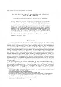
In most approaches, closed form functions are used to express the relationship among the variables, although the newer method of neural networks substitutes an empirical “black box” for a function. Fitting closed form equations to data is useful for analysis and interpretation of the observed quantities. It helps in judging the strength of the relationship between the independent (predictor) variables and the dependent (response) variables, and enables prediction of dependent variables for new values of independent variables. Although curve fitting problems were first introduced almost three centuries ago [25], there is still no single methodology that can be applied universally. This is partially due to the diversity of the problem areas, and particularly due to the computational limitations of the various approaches that deal with only subsets of this broad scope. Linear regression, spline fitting and autoregressive analysis are all solution methodologies to system identification and curve fitting problems. 2. HIERARCHICAL GENETIC APPROACH In the approach of this paper, the primary objective is to identify an appropriate functional form and then estimate the values of the coefficients associated with the functional terms. In fact, the entire task is a continuous optimization process in which a selected error metric is minimized. A hierarchical approach was used to accomplish this sequentially as shown in Figure 1. The upper genetic algorithm (GA) selects candidate functional forms using a pool of the independent variables and user defined functional primitives. The functions are sent to the lower (subordinate) GA which selects the coefficients of the terms of each candidate function. This selection is an optimization task using the data set and difference between the actual and fitted y values.
2
Upper Module
Function and Variable Selection + Ccos y = Cx ( C3 + C4 x22 ) 2 1 1 candidate functions
Lower Module
optimized coefficients for functions
Coefficient Estimation y = 9.234 x1 − 2.123cos (0.093 + 4.823x22 ) SSE = 0.34627 Figure 1 Hierarchical GA Framework
GA has been applied to system identification and curve fitting by several researchers. The relevant work on these can be categorized into two groups. The first category includes direct adaptation of the classical GA approach to various curve fitting techniques [17, 23]. In these works GA replaces traditional techniques as a function optimization tool. The second category includes more comprehensive approaches where not only parameters of the model, but the model itself, are search dimensions. One pioneering work on this area is Koza’s adaptation of Genetic Programming (GP) to symbolic regression [18]. The idea of genetically evolving programs was first implemented by [8, 12]. However, GP has been largely developed by Koza who has done the most extensive study in this field [18, 19]. More recently, Angeline used the basic GP approach enhanced with adaptive crossover operators to select functions for a time series problem [1].
3
3. COEFFICIENT ESTIMATION (LOWER GA) The approach consists of two independently developed modules which work in a single framework. The lower GA works as a function call from the upper one to measure how well the selected model fits the actual data. In the lower GA, the objective is to select functional term coefficients which minimize the total error over the set of data points being considered. A real value encoding is used. The next sections describe population generation, evolution, evaluation, selection, culling and parameter selection. 3.1 The Initial Population Using the example of the family of curves given by equation 1, there are two variables, x1 and x2, and four coefficients. Therefore each solution (population member) has four real numbers, C1, C2, C3, C4. y = C1 + C2 x13 + C3 cos x 2 + C4 x1 x 2
(1)
The initial estimates for each coefficient are generated randomly over a pre-specified range defined for each coefficient. The specified range need not include the true value of the coefficient (though this is beneficial). The uniform distribution is used to generate initial coefficient values for all test problems studied in this paper, although this is not a requirement either (see [15] for studies on diverse ranges and other distributions). 3.2 Evolution Mechanism A fitness (objective function) value which measures how well the proposed curve fits the actual data is calculated for each member of the population. Squared error is used here (see [15] for
4
studies on absolute error and maximum error). Minimum squared error over all data points results in maximum fitness. Parents are selected uniformly from the best half of the current population. This is a stochastic form of truncation selection originally used deterministically in evolution strategies for elitist selection (see [2] for a good discussion of selection in evolution strategies). Mühlenbein and Schlierkamp-Voosen later used the stochastic version of truncation selection in their Breeder Genetic Algorithm [20]. The values of the offspring’s coefficients are determined by calculating the arithmetic mean of the corresponding coefficients of two parents. This type of crossover is known as extended intermediate recombination with α = 0.5 [20]. For mutation, first the range for each coefficient is calculated by determining the maximum and minimum values for that particular coefficient in the current population.
Then the
perturbation value is obtained by multiplying the range with a factor. This factor is a random variable which is uniformly distributed between ±k coefficient range. The value of k is set to 2 in all test problems in this paper. However, the range among the population generally becomes smaller and smaller during evolution. In order to prevent this value from becoming too small, and thus insignificant, a perturbation limit constant, ∆ , is set. This type of mutation scheme is related to that used in Mühlenbein and
Schlierkamp-Voosen's Breeder Genetic Algorithm [20].
However their range was static where the range in this approach adapts according to the extreme values found in the current population with a lower bound of ∆. Mutation is applied to M members of the population, which are selected uniformly. After mutation and crossover, the newly generated mutants and offspring are added to the population and the lowest ranked members are culled, maintaining the original population size, ps.
5
Cycle length, cl, is used as a basis for terminating the search process. It refers to the number of generations without any improvement in the fitness value prior to termination. If the algorithm fails to create offspring and mutants with better fitness values during this fixed span of generations, the search process is automatically terminated. 3.3 Parameter Selection The lower GA was examined at various population parameters, namely population size ps, number of mutants M, number of offspring O, perturbation limit constant ∆ and cycle length cl, as shown in Table 1. The experimental design covered a wide range of values and a full factorial experiment was performed. Table 1 Evolution Parameter Levels for the Lower GA Level
ps
O
M
∆
cl
Low
30
10
5
10-6
10
10-5
50 100
Medium 50
20
10
-4
10
500
10-3
1000 2000
High
100 50
20
10-2
5000
Based on experimental test results, ps = 30, O = 10, M = 10 ∆ = 10 −5 and cl = 100 were selected for the lower GA. The strategy in selecting ∆ and cycle length is based on selecting the maximum ∆ value and minimum cycle length provided that the algorithm satisfies convergence criteria for all cases. Increasing ∆ or decreasing cl reduces computational effort, but it may also deteriorate the accuracy of the final results. An opposite strategy, decreasing ∆ or increasing cl improves accuracy, but it will take the algorithm more effort to converge to the final results.
6
3.4 Test Problems Since the lower GA module was initially developed independently from the framework, it was tested on three test problems where the correct functional form is provided. Two of these three test problems were taken from previous GA studies on curve fitting. The first test problem is to estimate the value of two coefficients (C1 and C2) of the straight line given in equation 2. This was studied by [17] with their GA approach.
y = C1 x + C2
(2)
The second test problem, which is given in equation 3, has 10 independent variables and 9 coefficients to be estimated. This was studied for spline fitting using a GA by [23] and, before that, for conventional spline fitting by [11]. A set of 200 randomly selected data points was used, and the problem was designed so that the response depends only on the first five variables. The remaining variables, x6 through x10, have no effect on the response function, and they are included in the data set as misleading noise. Therefore the optimal values of C5 through C9 should be zero. 10
y = C1 sin(π x1 x 2 ) + C2 ( x 3 − 0.5)2 + C3 x 4 + C4 x 5 + ∑ Cn−1 x n
(3)
n= 6
The third test problem is a general second level equation of three variables. The function, which is given in equation 4, has 10 coefficients to be estimated, and it is larger and more complex than any that can be found in the previous literature on using genetic algorithms for coefficient estimation. y = C1 + C2 x1 + C3 x 2 + C4 x 3 + C5 x12 + C6 x 22 + C7 x 32 + C8 x1 x 2 + C9 x1 x 3 + C10 x 2 x 3
(4)
7
The performance of the lower GA was tested with respect to data set size, population distribution and interval for sampling, error metric, initial coefficient range and random seeds. Robust performance was observed for all of the above parameters and performance exceeded previous approaches in terms of minimization of error (for details see [15]). The lower GA is highly flexible, and it can be adopted to different problem instances and parameters with very minor modifications in the algorithm. The coefficient optimization module is used as a subroutine to the function identification module described in the next section. 4. FUNCTIONAL FORM SELECTION (UPPER GA) Although the desire to develop a heuristic method to select the functional form was expressed in the literature as early as 1950s, it was suggested as a possible extension of variable selection in stepwise regression [7, 9, 28]. In the approach of this paper, a very liberal selection procedure is used so that the search domain is open to all possible functional forms, but can also be restricted by the user. 4.1 Encoding In terms of GA parlance, each member of the population set is a closed form function. Since the elements of the population are not simple numeric values, a binary array representation is not applicable. Instead, a tree structure is used to represent each closed form function. As an example, the tree structure for the candidate solution given below (equation 5) is illustrated in figure 2. y = 3.2 + 7.5 x13 + 1.6 cos( −4.1x 2 ) + 4.6 x1 x 2
(5)
8
The nodes in a tree structure can be categorized into two groups according to the number of outgoing branches: the “terminal node” is the last node in each branch without any outgoing branches. The nodes between the first and terminal nodes are called “intermediate nodes”, and they have at least one outgoing branch. Each intermediate node has an operand (e.g., sin, cos, exp, ln, +, ×) and the terminal node carries a variable or a constant. The numbers beside nodes in figure 2 are real valued coefficients (obtained from the lower GA). +
+
1
+
1.6 cos
*
*
3.2 *
x1
x1
1.0
3.0
x1
x2
x1
2.5
-4.1
9.2
0.5
Figure 2 Tree Structure Representation of Equation 5 Each tree structure has a starting node where branching is initiated. The number of branches originating from a node is determined probabilistically, restricted to 0, 1 or 2. The only exception is the first node where there must be at least one branch in order to initiate the generation of the tree structure. The branches connecting the nodes also determine the “parentoffspring relation” between the nodes. For a branch coming out of node a and going into node b, node a is named the parent of node b. In a similar manner, node b is called a child of node a. Each parent node can have one or two child nodes. It is also possible that the parent may not 9
have a child. If a node has two children, they are respectively called the left-child and the rightchild. However, if a node has only one child, it is still called the left-child. For computational reasons, such as the fitness calculation, the nodes are indexed. The indexing process starts from the first node, which is indexed as 1. At this point the number of children are also calculated for the node. Then the process moves, first to the left-child of the current node (now the child becomes a parent), and indexes it as 2. This process continues until a node is reached with no left-child. In such a situation the process backups to the parent node and looks for a right-child. If parent has a right-child which is not indexed yet, then it is indexed. Otherwise, the procedure climbs up to next parent (or grandparent). This recursive process, which is analogous to a “depth first search” algorithm, stops when all the nodes are indexed. Figure 3 illustrates the tree structure of figure 2 which is indexed according to this procedure. 1
9
2
3
10
4
5
6
8
11
12
13
14
7
Figure 3 Indexing of a Tree Structure The number of branches from a node will be Pr(B1, B2, B3) where B1, B2 and B3 represent the probability of having 0, 1 or 2 offspring nodes respectively. Special attention should be paid when assigning values for B1, B2 and B3. For example if B1, B2 and B3 are selected as 0.2, 0.4 and 10
0.2, each node, on the average, will have 0.2 × 0 + 0.4 × 1 + 0.2 × 2 = 1.2 offspring nodes. With such a number for the mean number of offspring nodes, it is possible to have tree structures with less than 10 or 15 nodes. However, it is also possible that tree structures which have tens or hundreds of nodes will be created. To remedy this, B1, B2 could be increased and B3 decreased. However, this will create deep structures which will reduce the efficiency of representing the functional forms.
As a remedy, the values of B1, B2 and B3 change during the course of
branching. At the early stages, there is a higher probability for double branching which diminishes gradually as the number of nodes increase. This is done by choosing a factor, δ , that is equal to 0.04 × index number. The δ value is added to B1, and it is subtracted from B3 at each node. As the number of nodes becomes larger, the probability of double branching decreases with respect to the probability of no branching. One dimensional arrays were used to store the tree structures. The following information is stored for each node: (1) index number, (2) number of offspring nodes, (3) index number of left child node, (4) index number of right child node, (5) index number of parent node, (6) type of functional primitive assigned to the node, and (7) whether the node carries a coefficient or not. 4.2 Functional Primitives The functional primitives are categorized into three hierarchical groups. The lowest level includes the independent variables of the data set and the constant 1. These are assigned only to terminal nodes and all carry a coefficient. If the variable x is assigned to a node and has coefficient value of 4.3, then it corresponds to 4.3x.
Similarly, a node with constant 1 and coefficient -2.3
corresponds to -2.3×1 = -2.3. The second and third groups include unary and binary operators respectively. While operators such as sin, cos, ln, exp, are categorized as second group operators,
11
multiplication “×”, division “÷”, and addition “+” operators form the third group (table 2). Functional primitives can be customized by the user according to estimated characteristics of closed form representation and the desired restrictiveness of the search. The assignment of primitives to the nodes is carried out in the following manner: the first group elements xn and the constant 1 are assigned to terminal nodes where there is no outgoing branch. The unary operators are assigned to nodes with a single outgoing branch and the binary operators are assigned to nodes with two outgoing branches. Each of the first and second group operators is proceeded by a coefficient. The third group operators do not have a coefficient preceding them, because they simply combine two sub-functions which already have coefficients. Table 2 Node Primitives Levels
Primitives*
First Group
x1,...,xn, 1
Second Group (unary)
sin, cos, exp, ln
Third Group (binary)
+, ×, ÷
*n is the number of independent variables in the data set 4.3 Initial Population and Fitness The initial population is randomly created in three stages. In the first stage, the tree structure is developed for each member of the population. At the second stage, appropriate primitives are assigned to the nodes in a random manner. After the functional form representation is obtained for the initial population, the fitness value of each member is calculated.
The coefficient
estimation process is done by the subordinate GA program, which is used as a function call in the main program. Two metrics are used for fitness: the first one is the raw fitness, which is the sum of squared errors.
The second fitness value is developed to penalize complex functional
12
representations in order to prevent overfitting. This secondary fitness value, called “penalized fitness”, is calculated by worsening the raw fitness in proportion to the complexity of the closed form function. The complexity of a closed form function is determined by the number of nodes it has. However complexity is not a absolute concept and the user needs to judge the level of complexity for each data set.
The objective is to balance the bias and variance in a closed form
representation, where bias results from smoothing out the relationship and variance indicates dependence of the functional form on the exact data sample used [14]. Ideally, both bias and variance will be small. A penalty function with user tunable parameters is used to balance bias and variance of the functional form in the GA approach. The penalty is determined by dividing the number of nodes in the tree structure by a threshold, T, and then taking the ( P) th power of the quotient (equation 6), where 0