1
Genetic Programming for System Identification Janos Madar, Janos Abonyi and Ferenc Szeifert University of Veszprem, Department of Process Engineering, P.O. Box 158, H-8201, Hungary, e-mail:
[email protected], http://www.fmt.vein.hu/softcomp
Abstract— Linear in parameter models are quite widespread in process engineering, e.g. NAARX, polynomial ARMA models, etc. This paper proposes a new method for nonlinear structure selection for linear in parameter models. The method uses Genetic Programming (GP) to generate nonlinear input-output models represented in tree structure. The main idea of the paper is to apply Orthogonal Least Squares algorithm (OLS) to estimate the contribution of the branches of tree to the accuracy of the model. The proposed method speeds up the convergence of the GP and results in more robust and interpretable models. The simulation results show that the proposed tool provides an efficient and fast method to determine the order and the structure of nonlinear input-output models. Index Terms— Keywords: Structure identification, Genetic Programming, Orthogonal Least Squares, Linear in parameter models
I. I NTRODUCTION TO DATA -D RIVEN S YSTEM I DENTIFICATION This paper focuses on data-driven identification of dynamical systems. The data-driven identification of nonlinear dynamical systems involves the following tasks [1]: a, Structure selection. How to select the regressors (model order) and the structure of the nonlinear static functions used to represent the model. b, Input sequence design. Determination of the input sequence which is injected into the plant to generate the output sequence that can be used for identification. c, Noise modelling. Determination of the dynamic model which generates the noise. d, Parameter estimation. Estimation of the model parameters from the input-output sequence. e, Model validation. Comparison of the output of the plant and the model based on data not used in model development. Most data-driven identification algorithms assume that the model structure is a priori known or that it is selected by a higher-level ‘wrapper’ structure-selection algorithm. Several information-theoretic criteria have been proposed for structure selection in linear dynamic input-output models. Examples of the classical criteria are the Final Prediction-Error (FPE) and the Akaike Information Criterion (AIC) [2]. Later, the Minimum Description Length (MDL) criterion developed by Schwartz and Rissanen was proven to produce consistent estimates of the structure of linear dynamic models [3]. With these tools, determining the structure of linear systems is a rather straightforward task.
Relatively little research has been done into the structure selection for nonlinear models. In the paper of Aguirre and Billings [4], the concepts of term clusters and cluster coefficients are defined and used in the context of system identification. It is argued that if a certain type of term in a nonlinear model is spurious, the respective cluster coefficient is small compared with the coefficients of the other clusters represented in the model. In [5], this approach is used to the structure selection of polynomial models. In [6] an alternative solution to the model structure selection problem is introduced by conducting a forward search through the many possible candidate model terms initially and then performing an exhaustive all subset model selection on the resulting model. A backward search approach based on orthogonal parameterestimation is also applied [7], [8]. It should be bore in mind that there is no escape of performing a model-driven structure selection, once a certain model representation is chosen. For instance, suppose a modelfree model order selection algorithm is used to determine the correct model order. If a neural network is used to model the process, the designer still need to decide on the activation function, the number of nodes etc. Therefore, the model order selection method that will be presented in this paper definitely not spare the user of having to go through some sort of structure selection. In this paper we propose a structure selection method for nonlinear models that are linear in parameters. This method is based on the Genetic Programming (GP) and the Orthogonal Least Squares (OLS) algorithm. In Section II the linear in parameter models and the OLS are presented, in Section III a modified GP algorithm is presented which is suitable for linear in parameter models and polynomial models. Finally in Section V the application examples are shown. II. L INEAR IN PARAMETER M ODELS A. Introduction to Linear in Parameter Models Many general nonlinear model structures (like neural networks) lead to a large number of parameters that has to be estimated based on the available input-output data. In some cases the excessive number of unknown coefficients leads to ill-conditioned estimation problem causing numerical difficulties and high sensitivity to measurement errors. Furthermore, nonlinear optimization algorithms used to the identification of these parameters may stuck in a local minima. To handle these difficulties this paper proposes the linear in parameter models.
2
A nonlinear single-output discrete model can be formulated as yˆ(k) = F (x(k), p) .
(1)
where y(k) is the output at the k-th time instant, x(k) is the input of the model at the k-th time instant, f is a nonlinear function, p is the parameter vector. The linear in parameter models are such nonlinear models which linear with respect to model parameters: yˆ(k) =
M X
pi Fi (x(k)) ,
where N is the number of data-points. Hence the optimal p = [p1 , . . . , pM ] parameter vector, where the χ2 is minimal, can be calculated by LS method: ¡ ¢ p = F−1 F FT y, (6) where y = [y(1), . . . , y(N )] is the measured and the F regression matrix is: F1 (x(1)) . . . FM (x(1)) .. .. .. F= . . .
(2)
F1 (x(N )) . . . FM (x(N ))
where F1 , . . . , FM are nonlinear functions, and p1 , . . . , pM denote model parameters. As it is known, the Gabor–Kolmogorov Analysis of Variance (ANOVA) decomposition of a general nonlinear function results in linear in parameters model:
C. Orthogonal Least Squares (OLS) Algorithm
output vector, .
(7)
i=1
f (x) ' f0 +
n X
fi (xi ) +
i=1
n n X X
fij (xi , xj ) + · · ·
i=1 j=i+1
+f1,2,...,n (x1 , . . . , xn ),
(3)
where the f (x) function is approximated by an additive decomposition of simpler subfunctions; in which f0 is a bias term and fi (xi ), fij (xi , xj ), . . . represent univariate, bivariate, . . . components. Any function, and hence any reasonable dynamical system can be represented by this decomposition. It means that the most of dynamical systems can be modelled well by linear in parameter models. This paper focuses on input-output models, where the input vector of model (2), consists of the lagged u inputs, y outputs, and e modelling errors: x(k) = (u(k − nd − 1), · · · , u(k − nd − nu ), y(k − nd − 1), · · · , y(k − nd − ny ), e(k − nd − 1), · · · , e(k − nd − ne )).
(4)
The nd is the dead-time, the nu , ny and ne are the input, output- and error-order, respectively. With the use of this definition all the linear in parameter models that are used in process engineering can be obtained, such as Nonlinear Additive AutoRegressive models (NAARX) [9], Volterra models Polynomial ARMA models [10]. The aim of this paper is to present an efficient method for the data-driven selection of the model order (nd , nu , ny and ne ) and the structures of models that are member of these model classes. B. Least Squares Method (LS) The great advantage of linear in parameter models is that the Least Squares Method (LS) can be used for the identification of the parameters, which is much less computationally demanding than nonlinear optimization algorithms. The LS method minimizes the square error between measured and calculated output à ! N M X X 2 χ = y(k) − pi Fi (x(k)) , (5) k=1
i=1
Most of the systems certain input interactions will be redundant and hence components in the ANOVA decomposition can be ignored which results in a more parsimonious representation. The OLS algorithm [11], [12] is an effective algorithm to determine which terms are significant in a linear in parameter model. The OLS introduce the error reduction ratio (err) which is a measure of the decrease in the variance of output by a given term. The compact matrix form corresponding to the linear in parameter model (2) is y = Fp + e,
(8)
where the F is the regression matrix (7), p is the parameter vector, e is the error vector. The OLS technique transforms the columns of F matrix (7) into a set of orthogonal basis vectors in order to inspect the individual contribution of each terms. Assume that the regression matrix F can be orthogonally decomposed as F = WA, where A is an M × M unit triangular matrix and W is an N × M matrix with orthogonal columns in the sense that WT W = D diagonal matrix. (N is the length of y vector, M is the number of regressors.) After that one can calculate the OLS auxiliary parameter vector g as g = D−1 WT y, (9) where gi is the corresponding element of the OLS solution vector. The output variance (yT y)/N can be explained as yT y =
M X
gi2 wiT wi + eT e.
(10)
i=1
Thus the error reduction ratio, [err]i of Fi term can be expressed as g 2 wT wi [err]i = i Ti . (11) y y This ratio offers a simple mean for ordering the terms, and it can be easily used to select the significant model terms. D. Model Structure Selection for Linear in Parameter Models The problem of model structure selection for linear in parameter models is to find the appropriate nonlinear Fi functions (2). There are two main methods for this problem: • The first method generates all of the possible model structures and selects the best.
3
The second method transforms this problem into an optimization problem, and solves it based on a (heuristic) search algorithm. The bottleneck of the first method is that there is a vast number of possible structures, hence, in practice, it is impossible to evaluate all of them. Even, if the set of the possible structures is restricted to polynomial models:
terminals are selected from a set of functions (operators) and a set of terminals. For example, the set of operators F can contain the basic arithmetic operations: {+, −, ∗, /}; however, it may also include other mathematical functions, Boolean operators, conditional operators or any user-defined operators. The set of terminals T contains the arguments for the functions. For example T = {y, x, pi } with x and y being two independent variables, and pi represents the parameters. m m m X X X Now, a potential solution (program) may be depicted as a y(k) = p0 + pi1 xi1 (k) + pi1 i2 xi1 (k)xi2 (k) rooted, labelled tree with ordered branches, using operations i1 =1 i1 =1 i2 =i1 n n m (internal nodes of the tree) from the function set and arguments X X Y +··· + ··· pi1 ···id xij (k), (12) (terminal nodes of the tree) from the terminal set. i1 =1 id =id−1 j=1 Generally, GP creates nonlinear models and not only linear the number of possible terms could be very large. If the in parameter models. To avoid nonlinear in parameter models number of regressors is m and the maximum polynomial the parameters are removed from the set of terminals, i.e. degree is d, the number of parameters (number of polynomial it contains only variables: T = {x1 (k), · · · , xm (k)}, where xi (k) denotes the i-th regressor variable. Hence a population terms) is np = (d+m)! d!·m! . E.g. if m = 5 and d = 3, the np = 56. In case of reasonable number of regressors (submodels) this member represents only the Fi nonlinear functions (2). The approach can be combined with OLS: the polynomial terms parameters are joined to the model after ’extracting’ the are sorted based on their error reduction ratio, and the best Fi functions from the tree, and they are determined using the LS method (6). One can ’extract’ Fi function terms by terms are selected. In the second method the structure selection problem is decomposing the tree starting from the root. On top of all, GP can be used with polynomial models. transformed into an optimization problem, in which the search space consists of possible structures. This method uses a To achieve it, one has to restrict the set of operators and search algorithm, which looks for an optimal structure. This introduce some simple syntactic rules. For example, if the set paper suggests using Genetic Programming algorithm to this of operators is defined as F = {+, ∗} and there is a syntactic rule that exchanges the internal nodes that are below a ’∗’-type task. internal node to ’∗’-type nodes, the algorithm will generate only polynomial models. III. G ENETIC P ROGRAMMING •
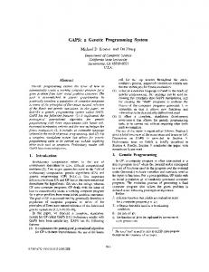
Genetic Programming is a symbolic optimization technique, developed by John Koza [13]. It is based on so called ”tree representation”. This representation is extremely flexible, since trees can represent computer programs, mathematical equations or complete models of process systems. This scheme has been already used for circuit design in electronics, algorithm development for quantum computers, and it is suitable for generating model structures: e.g. identification of kinetic orders [14], steady-state models [15], and differential equations [16]. A. Model Representation in GP Opposite to the common optimization methods, in which potential solutions are represented as numbers (vectors), in symbolic optimization algorithms, the potential solutions are represented by a structure of several symbols. One of the most popular method for representing structures is the binary tree; e.g. see Figure 1. + x1
x3
Fig. 1.
Genetic Programming is an Evolutionary Algorithm. It works with a set of individuals (potential solutions), and these individuals form a generation. In every iteration, the algorithm evaluates the individuals, selects individuals for reproduction, generates new individuals by mutation, crossover and direct reproduction, and finally creates the new generation. The initial step is the creation of an initial population. Generally it means generating individuals randomly to achieve high diversity. The first step is fitness evaluation, i.e. calculation of fitness values of individuals. Usually, the fitness value is calculated based on a cost function. After that, in the selection step, the algorithm selects the parents of the next generation and determines which individuals survive from the current generation. The most widely used selection strategy is the roulette-wheel selection, we used this strategy in this work. In the roulette-wheel selection, every individual has a probability to be selected as parent, and this probability is proportional to fitness value: pi = Pfi fi
/ x1
+
B. Genetic Operators
x2
A tree structure for the model: y = x1 + (x3 + x2 )/x1
A population member in GP is a hierarchically structured tree consisting of functions and terminals. The functions and
When an individual is selected for reproduction, three operations can be applied: direct reproduction, mutation and crossover (recombination). The probability of mutation is pm , the probability of crossover is pc , and the probability of direct reproduction is 1 − pm − pc . The direct reproduction puts the selected individual into the new generation without any change. In mutation a random change is performed on the selected tree structure by a random substitution. If an internal
4
element (an operator) is changed to a leaf element (an argument), the structure of tree will change too. In this case, one has to pay attention to the structure of the tree to avoid badformed binary trees. In crossover two individuals are selected, and their tree structure are divided at a randomly selected crossover point, and the resulting sub-trees are exchanged to form two new individuals. There are two types of crossover, one-point and two-point crossover. In one-point crossover, the same crossover point selected for the two parent-trees, in twopoint crossover, the two parent-trees are divided at different points. Before new individuals inserted to the population, it is necessary to ’kill’ the old individuals. We applied elitist replacement strategy in order to keep the best solutions with a ’generation gap’ Pgap parameter. E.g. the Pgap = 0.9 means that 90% of population is ’killed’ and the only the best 10% will survive.
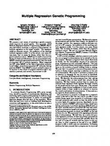
During the operation of GP, it generates a lot of potential solutions in the form of a tree-structure. These trees may have better and worse terms (subtrees) that contribute more or less to the accuracy of the model represented by the tree. The main idea of this paper is to apply OLS to estimate the contribution of the branches of the tree to the accuracy of the model. As it has been shown in Section II-C, with the use of OLS one can select the less significant terms in a linear regression problem. Terms having smallest error reduction ratio could be eliminated from the tree. The Figure 2 illustrates an example: the original tree contained three functions: F1 , F2 and F3 , these functions were put order based on OLS and then we decided to eliminate the F1 from the tree. + +
C. Fitness Function
where fi is the calculated fitness value, ri is the correlation coefficient, Li is the size of the tree (number of nodes), a1 and a2 are parameters of penalty function. In practice, a model which gives good prediction performance on the training data may be over-parameterized and may contain unnecessary, complex terms. The penalty function (13) handles this difficulty, because it decreases fitness values of trees that have complex terms. However, parameters of this penalty term are not easy to determine and the penalty function does not provide efficient solution for this difficulty. An efficient solution may be the elimination of complex and unnecessary terms from the model. For linear in parameter models it can be done by the Orthogonal Least Squares (OLS) algorithm. In the next section a tool that implements this method will be presented. IV. GP-OLS-T OOLBOX A. GP and OLS To improve the GP algorithm, this paper suggests the application of OLS in the GP algorithm.
x2
x1 F1
Fig. 2.
x2
x2
x1 x1
* x1
x1
*
+ x1
*
The fitness function has two aspects, in the first hand it reflects the goodness of a potential solution from the viewpoint of the cost function, on the other hand, it reflects a selection probability. Usually, the fitness function is based on the square error between estimated and measured output. However, during symbolic optimization, it is worth using correlation coefficient instead of square error, as [17] suggests it. Because the GP can result in too complex models, we must balance the consistency against accuracy. A good model is not only accurate but simple, transparent and interpretable too. In addition, a complex model results in over-parameterized model, which decreases the general estimation performance of the model. Hence [15] suggests using a penalty term in the fitness function: ri fi = , (13) 1 + exp (a1 (Li − a2 ))
+ F2
F1
F3
F2
Elimination a sub-tree based on OLS
There are several possibilities to apply this pruning approach. The pruning of the tree can be done in every fitness evaluation; or it can be the basis of mutation and recombination. In this case the probability of the genetic operators is not identical in every nodes of the tree, but it is the function of the error reduction ratio assigned to the given branch. This approach ensures that the less significant branches will be mutated, and the most significants will be transferred to the other trees. In this work a simple pruning approach was used, and the algorithm eliminated the less significant branches in every fitness evaluation. B. The MATLAB GP-OLS Toolbox The proposed approach has been implemented in MATLAB that is the most widely applied rapid prototyping system [18]. The aim of the toolbox is the data-based identification of static and dynamic models. Beside these tasks the toolbox is suitable for model-order selection of dynamical input-output models, and can also be applied for static nonlinear equation discovery. At the development of the toolbox special attention has been given to the identification of input-output models. Hence, the generated model equations can be simulated to get one- and n-step ahead predictions. The toolbox is freeware, and it is downloadable from the website of the authors: www.fmt.veim.hu/softcomp. The toolbox has a very simple and user-friendly interface. The user should only define the input-output data, the set of the terminal nodes (the set of the variables of the model), in case of a dynamical system this means the maximum inputoutput model orders, select the set of the internal nodes (set of mathematical operators) and set some parameters of the GP. Based on our experiments we found that with the parameters given in Table I the GP is able to find good solutions for various problems. Hence these parameters are the default
5
parameters of the toolbox that have not modified during the simulation experiments presented in this paper. TABLE I PARAMETERS OF GP
IN THE APPLICATION EXAMPLES
Population size Maximum number of evaluated individuals Generation gap Type of crossover Probability of recombination Probability of mutation Probability of changing terminal– non-terminal nodes (vica versa) during mutation
50 2500 0.9 two-point 0.5 0.5 0.25
Since polynomial models play an important role in process engineering, in this toolbox there is an option of generating polynomial models. If this option is selected, the set of operators is defined as F = {+, ∗}, and after every mutation and cross-over, the GP algorithm validates the model structure whether it is in the class of polynomial models. If it necessary the algorithm exchanges the internal nodes that are below a ’∗’-type internal node to ’∗’-type nodes. This simple trick transforms every tree to a well-ordered polynomial model. The OLS evaluation is inserted into the fitness evaluation step. Before calculation of the fitness value of the tree, the OLS calculates the error reduction ratio of the branches of the tree, and the terms which have error reduction ratio bellow a threshold value are eliminated from the tree. With the help of the selected branches, the OLS estimates the parameters of the model represented by the tree. After that, this new individual proceeds on its way in the GP algorithm (fitness evaluation, selection, etc.). V. A PPLICATION E XAMPLES In this section, the application of proposed GP-OLS technique is illustrated. In the first example, a simple input-output model structure is identified. It illustrates that the proposed OLS method improves the performance of GP algorithm. In the second example, the model order of a continuous polymerization reactor is identified. A. Example I: Nonlinear Input-Output Model In the first example, we identify a simple nonlinear inputoutput model which is linear in parameters. The model is the following: y(k) = 0.8u(k − 1)2 + 1.2y(k − 1) − 0.9y(k − 2) − 0.2. (14) The aim of the experiment is the identification of the model structure from measurements. The measurements was generated by simulation of the system and 4% relative normal distributed noise was added to the output. Based on this data, the GP identified the model equation. During the identification process the function set F contained the basic arithmetic operations F = {+, −, ∗, /}, and the terminal set T contained the following arguments T = {u(k − 1), u(k − 2), y(k − 1), y(k − 2)}. During the identification, maximum five terms were allowed in one model. Based on the OLS method, the terms of every model equation were
sorted by error reduction ratio, and the terms that have smaller reduction ratio than the limitation parameter were eliminated above the limitation. Three different approaches were compared: • Method 1.: GP without penalty function and OLS. • Method 2.: GP with penalty function and without OLS. • Method 3.: GP with penalty function and OLS. The Table II illustrates the results. Because GP is a stochastic method 10-10 runs were performed for each of methods. TABLE II R ESULTS OF E XAMPLE I. (10-10 RUNS FOR EVERY METHOD ) Method Found perfect solution Found non-perfect solution Average runtime
1 0 10 1000
2 6 4 880
3 7 3 565
The Method 3. proved the best, it was able to find the perfect model structure at 7 times, and it find the perfect structure in the smallest time; thanks to the OLS technique. B. Example II: Continuous Polymerization Reactor In the first example the identified model structure was perfectly known. In this experiment, a perfect model structure does not exist, but the correct model order is known. This experiment demonstrates that the proposed GP-OLS technique is able to find the correct model order for polynomial models. The example is taken from [19], the input-output data is generated by a simulation model of a continuous polymerization reactor. This model describes the free-radical polymerization of methyl-methacrylate with azo-bis(isobutyro-nitrile) as an initiator and toluene as a solvent. The reaction takes place in a jacketed CSTR. The first-principle model of this process is given in [20]. The dimensionless state variable x1 is the monomer concentration, and x4 /x3 is the number-average molecular weight (the output y). The process input u is the dimensionless volumetric flow rate of the initiator. According to [19], we apply a uniformly distributed random input over the range 0.007 to 0.015 with the sampling time of 0.2 s. The first-principle model has four states, however the system has two states that are weakly observable. This week observability leads to the system can be approximated by a small input–output description [21]. This is in agreement with the analysis of Rhodes [19] who showed that a nonlinear model with m = 1 and n = 2 orders is appropriate; in other words the model can be write in the next form: y(k) = G (y(k − 1), u(k − 1), u(k − 2)) ,
(15)
if the discrete sample time T0 = 0.2. In this example we examined four methods: • Method 1.: It generates all of the possible polynomials with degree d = 2. The model consists of all of these terms. • Method 2.: It generates all of the possible polynomials with degree d = 2, but the model only consists of the terms which have greater error reductions ratios than 0.01.
6
TABLE III R ESULTS OF E XAMPLE II. Method-1 Free-run mse One-step mse
Inf 7.86
Method-2
Method-3 min mean max 26.8 1.65 10.2 23.7 30.3 1.66 9.23 22.1 Remark: MSE in 10−3
Method 3.: Polynomial GP-OLS technique. The operator set is F = {∗, +}. The OLS threshold value is 0.02. • Method 4.: Non-polynomial GP-OLS technique. The op√ erator set is F = {∗, +, /, }. The OLS threshold value is 0.02. The Table III shows the mean square errors (mse) of resulted models for one-step ahead prediction and for free-run prediction. The GP is stochastic algorithm, so we performed 10 experiments for third and fourth method, and the table contains the minimum, the maximum and the mean of resulted mse values. The input and output order were limited to four: u(k − 1), · · · , u(k − 4), y(k − 1), · · · , y(k − 4). In the first method, the model consisted of 45 polynomial terms (m = 8, d = 2). This model was very accurate for one-step ahead prediction, but it was unstable in free-run prediction. Hence this model can not be used in free-run simulation. In the second method, the error reduction ratios were calculated for the 45 polynomial terms, and the terms which have very small values (below 0.01) were eliminated. After that, only three terms remained: y(k) = u(k − 1) + y(k − 1) + y(k − 2). This model is simple linear model, it was stable in free-run, but it was not accurate. The third method resulted different models, due to its stochastic nature, in the 10 experiments. All of resulted models were stable in free-run. The most accurate model was y(k) = u(k − 1) ∗ u(k − 1) + y(k − 1) + u(k − 2) + u(k − 1) ∗ y(k − 1) which has correct model order (see (15)). This methods found the correct model order in six cases from the ten. The fourth method (GP-OLS) resulted correct model orders in three cases from the ten. This method found the most accurate model, and all of resulted models were stable in freerun. Some of the resulted models were the same that the third method generated. Statistically this method generated the most accurate models, but the third method was better at finding the correct model order. •
VI. C ONCLUSIONS This paper proposes a new method for nonlinear structure selection for linear in parameter models. The method uses Genetic Programming (GP) to generate nonlinear input-output models represented in tree structure. The main idea of the paper is to apply Orthogonal Least Squares algorithm (OLS) to estimate the contribution of the branches of the tree to the accuracy of the model order. The GP-OLS algorithm generates linear in parameter models or polynomials models, and the simulation results show that the proposed tool provides an efficient and fast method for selecting input-output model structure for nonlinear processes.
min 0.95 0.84
Method-4 mean max 7.15 20.6 6.63 17.8
R EFERENCES [1] L. Ljung. System Identification, Theory for the User. Prentice–Hall, New Jersey, 1987. [2] H. Akaike. A new look at the statistical model identification. IEEE Trans. Automatic Control, 19:716–723. [3] G. Liang, D.M. Wilkes, and J.A. Cadzow. Arma model order estimation based on the eigenvalues of the covariance matrix. IEEE Trans. on Signal Processing, 41(10):3003–3009, 1993. [4] L.A. Aguirre and S.A. Billings. Improved structure selection for nonlinear models based on term clustering. International Journal of Control, 62(3):569–587, 1995. [5] L.A. Aguirre and E.M.A.M. Mendes. Global nonlinear polynomial models: Structure, term clusters and fixed points. International Journal of Bifurcation and Chaos, 6(2):279–294, 1996. [6] E.M.A.M. Mendes and S.A. Billings. An alternative solution to the model structure selection problem. IEEE Transactions on Systems Man and Cybernetics part A-Systems and Humans, 31(6):597–608, 2001. [7] M. Korenberg, S.A. Billings, Y.P. Liu, and P.J. McIlroy. Orthogonal parameter-estimation algorithm for nonlinear stochastic-systems. International Journal of Control, 48(1):193–210, 1988. [8] J. Abonyi. Fuzzy Model Identification for Control. Birkhauser: Boston, 2003. [9] R.K. Pearson and B.A. Ogunnaike. Nonlinear process identification. In M.A. Henson and D.E. Seborg, editors, Nonlinear Process Control, pages 11–109. Prentice–Hall, Englewood Cliffs, NJ, 1997. [10] E. Hernandez and Y. Arkun. Control of nonlinear systems using polynomial arma models. AICHE Journal, 39(3):446–460, 1993. [11] S.A. Billings, M. Korenberg, and S. Chen. Identification of nonlinear output-affine systems using an orthogonal least-squares algorithm. International Journal of Systems Science, 19(8):1559–1568, 1988. [12] S. Chen, S.A. Billings, and W. Luo. Orthogonal least squares methods and their application to non-linear system identification. International Journal of Control, 50(5):1873–1896, 1989. [13] J.R. Koza. Genetic Programming: On the programming of Computers by Means of Natural Evolution. MIT Press, Cambridge, 1992. [14] L. Kang Y. Chen H. Cao, J. Yu. The kinetic evolutionary modeling of complex systems of chemical reactions. Computers and Chem. Eng., 23:143–151, 1999. [15] B. McKay, M. Willis, and G. Barton. Steady-state modelling of chemical process systems using genetic programming. Computers and Chem. Eng., 21(9):981–996, 1997. [16] E. Sakamoto and H. Iba. Inferring a system of differential equations for a gene regulatory network by using genetic programming. In Proceedings of the 2001 Congress on Evolutionary Computation CEC2001, pages 720–726, COEX, World Trade Center, 159 Samseong-dong, Gangnamgu, Seoul, Korea, 2001. IEEE Press. [17] M.C. South. The application of genetic algorithms to rule finding in data analysis, PhD. thesis. Dept. of Chemical and Process Eng., The Univeristy of Newcastle upon Tyne, UK, 1994. [18] MATLAB Optimization Toolbox. MathWorks Inc.: Natick, MA, 2002. [19] C. Rhodes and M. Morari. Determining the model order of nonlinear input/output systems. AIChE Journal, 44:151–163, 1998. [20] F.J. Doyle, B.A. Ogunnaike, and R. K. Pearson. Nonlinear model-based control using second-order volterra models. Automatica, 31:697, 1995. [21] C. Letellier and L.A. Aguirre. Investigating nonlinear dynamics from time series: The influence of symmetries and the choice of observables. Chaos, 12(3):549–558, 2002.