2010 International Conference on Pattern Recognition
A Hierarchical GIST Model Embedding Multiple Biological Feasibilities for Scene Classification Yina Han, and Guizhong Liu School of Electronics and Information Engineering, Xian Jiaotong University, China
[email protected],
[email protected]
Abstract We propose a hierarchical GIST model embedding multiple biological feasibilities for scene classification. In the perceptual layer, spatial layout of Gabor features are extracted in a bio-vision guided way: introducing diagnostic color information, tuning the orientations and scales of Gabor filters, as well as the spacial pooling size to a biological feasible value. In the conceptual layer, for the first time, we attempt to build a computational model for the biological conceptual GIST by kernel PCA based prototype representation, which is specific task orientated as biological GIST, and also in accordance with the unsupervised learning assumption in the primary visual cortex and prototype similarity based categorization in human cognition. Using around 200 dimensions, our model is shown to outperform existing GIST models, and to achieve state-of-the-art performances on four scene datasets.
1. Introduction One of the most remarkable feats of human visual system is the ability to recognize a complex novel scene very rapidly and accurately [5]. Behavioral studies have shown that observers can rapidly capture the “gist” of the presented scenes without any attention [1, 12]. Hence building a reasonable computational model for GIST is critical for rapid and accurate scene classification. In general, GIST can be represented at both perceptual and conceptual levels [6]. Perceptual GIST refers to the spacial configuration of a scene built during perception [12], and has been modeled as average pooling of various biological relevant low-level features over nonoverlapping subregions arranged on a fixed grid [5, 6, 10]. However, from the biological feasible view, the above representation is inadequate, reflected in empirical filter parameters and pooling size. 1051-4651/10 $26.00 © 2010 IEEE DOI 10.1109/ICPR.2010.761
Conceptual GIST refers to the inferred semantic information from the perceptual level, which has not been clearly proposed in existing models [5, 6, 10]. Though their adopted dimension reduction technique (such as PCA/ICA) does encode some statistics, it has not sufficiently reveal the semantically related statistics. In this paper, we propose to improve GIST modeling using a hierarchical representation including both perceptual and conceptual layers. In the perceptual layer, we enrich the most widely used Gabor based model [6], which will be referred as OT-GIST, in several biological feasible aspects: introducing diagnostic color information, tuning the orientations and scales of Gabor filters, as well as the pooling size in a bio-vision guided way. Then, for the first time (to our knowledge), we attempt to build a computational model for the biological conceptual GIST by prototype based representation. Here, Kernel PCA is used to mine the semantic prototypes, which is specific task orientated as biological GIST [6], and also in accordance with the unsupervised learning assumption in the primary visual cortex [4] and prototype similarity based categorization in human cognition [7]. We demonstrate the efficacy of the proposed model through substantial evaluations.
2. The Hierarchical GIST Model The hierarchical structure including both perceptual and conceptual layers is the inherent property of biological GIST [6, 12]. In our model, perceptual layer is modeled based on OT-GIST [6] as shown in Fig. 1. Specifically, the image is first decomposed by a set of Gabor filters with 4 scales and 8 orientations; then, the output magnitude of each filter is pooled by averaging over 16 nonoverlapping subregions divided by a 4 × 4 grid. Having the biological relevance of GIST in mind, we further tune the Gabor parameters and the pooling size, as well as introduce color information based on related bio-vision studies instead of empirical values, to 3101 3113 3109
maximize the similarity between our representation and the responses of real cortex to visual information. In the conceptual layer, which has not been clearly modeled yet, we attempt to model it by the Kernel PCA technology based on the following consideration: the specific task orientated property of biological GIST [6], the unsupervised learning assumption in the primary visual cortex [4], and the prototype similarity based categorization in human cognition [7].
3. Perceptual Layer 3.1. Color opponent features Color information is a key diagnostic cue of scene categories [6]. Given a color image X, with r, g, and b being the red, green, and blue values, four broadlytuned color channels are created: R = r − (g + b)/2, G = g − (r + b)/2, B = b − (r + g)/2 and Y = r + g − 2(|r − g| + b). According to the color opponent theories [10], that neurons in cortex are excited by the differences between colors rather than each individual one, and such chromatic opponency exists for red/green (RG) and blue/yellow (BY ) pairs, our model represents each color image as one intensity channel and two “color double-opponent” channels: 1 (r(x, y) + g(x, y) + b(x, y)) 3 RG(x, y) = kR(x, y) − G(x, y)k I(x, y) =
BY (x, y) = kB(x, y) − Y (x, y)k
(2) (3)
The kernels of Gabor filters have been proven to be similar to the profile of cortical simple cell receptive fields [9], and can be defined as follows: σ2 kkµ,ν k − kkµ,ν 2 2σ e [eikµ,ν z − e− 2 ] (4) 2 σ where µ and ν define the orientation and scale, z = (x, y), k · k denotes the norm operator, and the wave vector kµ,ν is defined as: kµ,ν = kν eiφµ . kν is the modulation frequency. It has been shown that the frequency bandwidth of simple cells in the visual cortex is about one octave [9]. In order to ensure the decomposition of an image into aliasing negligible octaves, kν should be: kν = π/2ν ; ν ∈ {0, . . . , N − 1}. The number of scales N is determined by the image size. In our model, the images are rescaled to 256 × 256 squares irrespective of their aspect ratio, thereby N = log2 (256) = 8. φµ = µ4φ; µ ∈ {0, . . . M − 1} is the orientation
gµ,ν (z) =
k2 kzk2
that filters tuned to. It has been shown that the resolution of the orientation tuning ability of the human visual system is as high as 5◦ . Here we set 4φ = 9◦ , and the number of orientations M is 180◦ /9◦ = 20. In summary, we would use Gabor filters of eight different scales, ν ∈ {0, . . . , 7}, and twenty orientations, µ ∈ {0, . . . , 19}. For the case of color image, I, together with RG and BY is decomposed by the proposed Gabor filters respecitively:
(1)
3.2. Biological feasible Gabor filters
2
Figure 1. Perceptual layer overview
Ol,µ,ν (x, y) = l(x, y) ∗ gµ,ν (x, y)
(5)
where l ∈ {I, RG, BY }, µ ∈ {0, . . . , 19}, ν ∈ {0, . . . , 7}, and ∗ denotes convolution operator, resulting in 20 × 8 = 160 gray maps, and 2 × 20 × 8 = 320 color maps.
3.3. Resolution of spatial configuration For spatial layout information which is diagnostic in scene categorization [6], each map Ol,µ,ν (x, y); l ∈ {I, RG, BY }, µ ∈ {0, . . . , 20}, ν ∈ {0, . . . , 8} is pooled by averaging on nonoverlapping subregions arranged on a R × R grid, which can be formalized as: 2562 Gl,µ,ν (k, l) = R2
256(k+1) 256(l+1) −1 −1 R R
∑
∑
x= 256k R
y= 256l R
Ol,µ,ν (x, y)
(6) where k, l ∈ {1, . . . , R} are indices of the subregions. R controls the spatial resolution. Seeing that scene categories can be identified based on a resolution as low as 2 cycles/images in color, while 4 cycles/images in gray-scale [6], in our model we set R = 4 for color images and R = 8 for gray-scale images. Concatenating 3110 3114 3102
all Gl,µ,ν (k, l) forms the final “long” perceptual GIST vector, G p , namely 7680 dimensions for color images and 10240 dimensions for gray-scale images. The rich perceptual information is beneficial to further semantic inference in conceptual layer.
4. Conceptual Layer
Figure 2. Toy example for two tasks
4.1. Task-Wise Prototype Since our concern is the similarity measure and the eigenvector matrix V = (V1 , V2 , . . . , VM ) satisfies V = T HA, the l prototypes matrix for task Φ(T ), namely Vl = (V1 , V2 , . . . , Vl ), does not need to be computed explicitly. The l-dimensional concept Gxc an be directly inferred from perceptual Gxp as:
Since the content of GIST is constrained by categorization task [6], and categories are essentially defined by similarity to prototypes [7]. This requires to determine the most informative prototypes for each specific task as well as appropriate distance metric on the perceptual space, which is inherently non-linear and low dimensional [5]. Here we use KPCA [8] based method. Fig. 2 shows a toy example of the 2-D feature visualization (reduced by MDS) for two categorization tasks (indexed by rows) projected to four prototypes (indexed by columns), where colors represent similarities between features and prototypes.
˜ xp ) = AT HT T (Φ(Gxp ) − Φ) ¯ Gxc = VlT Φ(G 1 = AT H(kGxp − K1) l
(9)
c Specifically, each component Gx,i , i ∈ {1, . . . , l} of c vector Gx is computed as:
c Gx,i = (Vi · Φ(Gxp )) =
4.2. KPCA based prototype representation
l ∑
aik k(Gxp , Gkp )
(10)
k=1
Given a specific categorization task T = {G1p , G2p , p . . . , GM }, where Gip , i ∈ {1, . . . , M } represents the perceptual GIST feature from the training set, M is the number of training data. Generally, the topology within T is nonlinear. By nonlinearly mapping Φ, Φ(T ) can be decomposed linearly by PCA. Taking the first l most informative eigenvectors as the prototypes, which best explain the variance in Φ(T ), the first l principle components of any Φ(Gxp ) naturally measure the similarity to the prototypes by Cosine Distance. Within the KPCA methodology [8], the centered ker˜ corresponding to T is first defined as: nel matrix K ˜ j) = ((Φ(G p ) − Φ) ¯ · (Φ(G p ) − Φ)) ¯ K(i, i j p p ˜ ˜ = (Φ(G ) · Φ(G )) i
i
( )T where kGxp = k(Gxp , G1p )k(Gxp , G2p ) . . . k(Gxp , Glp ) , and the polynomial kernel with fractional power, k(x, y) = (x · y)d , 0 < d < 1, is adopted in our model.
5. Experiments The proposed GIST model is evaluated for both scene and object classification tasks. All the experiments are repeated ten times with randomly selected training and testing images. The final result is reported as the mean and standard deviation of each individual one. Categorization is done with a rbf SVM. First we carry out three groups of experiments on four scene datasets: OT [5], VS [11], FP [1] and LSP [3] following the same protocol as [5, 11, 1, 3] that is 100 images per class for training (except for sky/clouds in VS with 30 for training) and the rest for testing. The first group is to compare our model with other GIST models: OT1 [5], OT [6], RM [12], and SI [10], implemented as in [10]. The second group is to compare our model with two popular BoF based models: pLSA-BoF and SPM-BoF, implemented as in [3]. The third group is to compare our model directly with the reported results in [5, 1, 3, 11] on the same dataset. The detailed comparison results are shown in Table 1. Observe that the performances of OT1, OT, RM and SI are similar, which is consistent with [10], while
(7)
˜ p, Gp) = k(G i i ¯ = 1 ∑M Φ(G p ). It can easily be shown where Φ i i=1 M ˜ = HKH, where H = I− 1 11t is the centering that K M matrix, I is the M ×M identity matrix, 1 = (1, . . . , 1)T ˜ is further is an M × 1 vector. The symmetric matrix K decomposed as: ˜ = AΛAt K (8) where Λ = diag(λ1 , . . . , λM ) is a eigenvalue matrix with (λ1 ≥ λ2 ≥ · · · λM ). The column vector of A, namely ai = (ai1 , . . . , aiN )T is the eigenvector corresponding to λi . 3111 3115 3103
Model OT1-Gist OT-Gist RM-Gist SI-Gist pLSA-BoF SPM-BoF Authors Ours
Table 1. Comparison of scene categorization performances OT OT-4N OT-4M VS FP 82.8 ± 0.7 85.1 ± 1.0 90.2 ± 2.1 56.4 ± 5.3 74.8 ± 1.1 83.3 ± 0.8 86.2 ± 1.1 91.6 ± 1.9 59.8 ± 4.8 76.6 ± 0.9 81.5 ± 0.8 83.3 ± 0.8 88.3 ± 1.2 57.2 ± 4.5 71.3 ± 0.7 82.3 ± 0.7 84.6 ± 1.0 88.7 ± 1.1 58.1 ± 3.1 73.4 ± 0.7 70.4 ± 0.8 71.0 ± 0.7 81.8 ± 1.1 61.1 ± 3.4 65.9 ± 1.4 87.5 ± 0.7 86.9 ± 0.8 91.9 ± 0.6 66.6 ± 7.2 81.7 ± 0.4 83.7 [5] 89.0 [5] 89.0 [5] 74.1 [11] 65.2 [1] 88.7 ± 0.7 91.3 ± 1.2 95.7 ± 1.3 74.4 ± 4.3 81.5 ± 0.7
LSP 71.5 ± 0.7 72.0 ± 0.6 70.2 ± 0.7 71.2 ± 0.6 63.3 ± 1.2 76.8 ± 0.5 81.4 [3] 76.6 ± 0.4
References
our model achieves better performances, especially for VS dataset, which is more ambiguous in semantics [11]. This demonstrates the “gist” of a scene can be better captured by our model. Compared to BoF models, our implementation of SPM-BoF is not able to reproduce the results reported in [3] probably due to some engineering problem. Following our own baseline, our model achieves similar performances to the state-ofthe-art SPM-BoF. But as a global representation, our model is more compact (with around 200 dimensions) than local regions based SPM-Bof model (with 4200 dimensions). Moreover, the rbf SVM used for our model is more efficient than histogram intersection SVM for SPM-BoF model.
[1] L. Fei-Fei and P. Perona. A bayesian hierarchical model for learning natural scene categories. CVPR, pages 524– 531, 2005. [2] Y. Huang, K. Huang, L. Wang, D. Tao, T. Tan, and X. Li. Enhanced biologically inspired model. Computer Vision and Pattern Recognition, IEEE Computer Society Conference on, 0:1–8, 2008. [3] S. Lazebnik, C. Schmid, and J. Ponce. Beyond bags of features: Spatial pyramid matching for recognizing natural scene categories. CVPR, pages 2169–2178, 2006. [4] J. Mutch and D. G. Lowe. Object class recognition and localization using sparse features with limited receptive fields. International Journal of Computer Vision, 80(1):45–57, 2008. [5] A. Oliva and A. Torralba. Modeling the shape of the scene: A holistic representation of the spatial envelope. International Journal of Computer Vision, 42(3):145– 175, May 2001. [6] A. Oliva and A. Torralba. Building the gist of a scene: the role of global image features in recognition. Progress in brain research, 155:23–36, 2006. [7] E. Rosch. Natural categories. Cognitive Psychology, 4:328–350, 1973. [8] B. Sch¨olkopf, A. J. Smola, and K. R. M¨uller. Nonlinear component analysis as a kernel eigenvalue problem. Neural Computation, 10:1299–1319, 1998. [9] T. Serre, L. Wolf, S. Bileschi, M. Riesenhuber, and T. Poggio. Robust object recognition with cortex-like mechanisms. IEEE Transactions on Pattern Analysis and Machine Intelligence, 29:411–426, 2007. [10] C. Siagian and L. Itti. Rapid biologically-inspired scene classification using features shared with visual attention. IEEE Transactions on Pattern Analysis and Machine Intelligence, 29(2):300–312, Feb 2007. [11] J. Vogel and B. Schiele. Semantic modeling of natural scenes for content-based image retrieval. International Journal of Computer Vision, 72(2):133–157, 2007. [12] L. L. Walker and J. Malik. When is scene recognition just texture recognition. Vision Research, 44:2301– 2311, 2003. [13] L. Wolf, S. M. Bileschi, and E. Meyers. Perception strategies in hierarchical vision systems. CVPR, pages 2153–2160, 2006.
Table 2. Comparison on Caltech-101 15 training 30 training Model images/cat. images/cat. Serre et al. [9] 35 42 Mutch & Lowe [4] 51 56 Wolf et al. [13] 51.2 − Huang et al. [2] 49.8 ± 1.2 − OT-GIST 48.7 ± 1.0 56.1 ± 1.1 Ours 53.7 ± 0.8 60.6 ± 1.1
To further compare with other biologicallymotivated models with their directly reported results, we evaluate our model on the Caltech-101 [1] dataset with 101 object categories and 1 background. Following the standard setup, training on 15 and 30 images per category and testing on the rest. As shown in Table. 2, our model achieves slightly better performances. The above results have proved the validity of introducing statistical conceptual layer for modeling GIST. However, performances on dataset with indoor scenes, and especially on Caltech-101, are not satisfactory. Therefore, our next step is to build conceptual GIST with more discriminative properties. 3112 3116 3104