A Hierarchical Low-Rank Decomposition Algorithm

Received: Added at production

Revised: Added at production

Accepted: Added at production

DOI: xxx/xxxx

ARTICLE TYPE

A Hierarchical Low-Rank Decomposition Algorithm Based on Blocked Adaptive Cross Approximation Algorithms Yang Liu*1 | Wissam Sid-Lakhdar1 | Elizaveta Rebrova2 | Pieter Ghysels1 | Xiaoye Sherry Li1 1 Computational

Research Division, Lawrence Berkeley National Laboratory, Berkeley, CA, USA 2 Department of Mathematics, University of California, Los Angeles, CA, USA Correspondence *Yang Liu, Email: [email protected]

Summary This paper presents a hierarchical low-rank decomposition algorithm assuming any matrix element can be computed in 𝑂(1) time. The proposed algorithm computes rank-revealing decompositions of sub-matrices with a blocked adaptive cross approximation (BACA) algorithm, followed by a hierarchical merge operation via truncated singular value decompositions (H-BACA). The proposed algorithm significantly improves the convergence of the baseline ACA algorithm and achieves reduced computational complexity compared to the full decompositions such as rank-revealing QR decompositions. Numerical results demonstrate the efficiency, accuracy and parallel efficiency of the proposed algorithm. KEYWORDS: Adaptive cross approximation, singular value decomposition, rank-revealing decomposition, parallelization, multi-level algorithms

1

INTRODUCTION

Rank-revealing decomposition algorithms are important numerical linear algebra tools for compressing high-dimensional data, accelerating solution of integral and partial differential equations, constructing efficient machine learning algorithms, and analyzing numerical algorithms, etc, as matrices arising from many science and engineering applications oftentimes exhibit numerical rank-deficiency. Despite the favorable 𝑂(𝑛𝑟) memory footprint of such decompositions with 𝑛 and 𝑟 respectively denoting the matrix dimension (assuming a square matrix) and numerical rank (𝜖-rank), the computational cost can be expensive. Existing rank-revealing decompositions such as truncated singular value decomposition (SVD), column-pivoted QR (QRCP), CUR decomposition, interpolative decomposition (ID), and rank-revealing LU typically require at least 𝑂(𝑛2 𝑟) operations 1–4 . This complexity can be reduced to 𝑂(𝑛2 log 𝑟 + 𝑛𝑟2 ) by structured random matrix projection-based algorithms 3, 5 . In addition, faster algorithms are available in the following three scenarios. 1. When each element entry can be computed in 𝑂(1) CPU time with prior knowledge (i.e., smoothness, sparsity, or leverage scores) about the matrix, faster algorithms such as randomized CUR and adaptive cross approximation (ACA) 6–8 algorithms can achieve 𝑂(𝑛𝑟2 ) complexity. However, the robustness of these algorithms relies heavily on the matrix properties that are not always present in practice. 2. When the matrix can be rapidly applied to arbitrary vectors, algorithms such as randomized SVD, QR and UTV (T lower or upper triangular) 5, 9–11 can be utilized to achieve quasi-linear complexity. 3. Finally, given a matrix with missing entries, the decomposition can be constructed via matrix completion algorithms 12, 13 in quasi-linear time assuming incoherence properties of the matrices (i.e., projection of natural basis vectors onto the space spanned by singular vectors of the matrix should not be very sparse). This work concerns the development of a practical algorithm, in application scenario 1, that improves the robustness of ACA algorithms while maintaining reduced complexity for broad classes of matrices.

2

Yang Liu ET AL

It is well-known that the partially-pivoted ACA algorithm suffers from deteriorated convergence and/or early termination for non-smooth or sparse matrices 14 . Hybrid methods or improved convergence criteria (i.e., hybrid ACA-CUR, averaging, statistical norm estimation) have been proposed to partially alleviate the problem 15, 16 . This work proposes a blocked ACA algorithm (BACA) that extracts a block row/column per iteration to significantly improve convergence of the baseline ACA algorithms. Compared to the aforementioned remedies, the proposed algorithm provides a unified framework to balance robustness and efficiency. Upon increasing the block size, the algorithm gradually moves from ACA to ID. To further improve the robustness of BACA, the matrix is first subdivided into 𝑛𝑏 submatrices compressed via BACA, followed by a hierarchical merge algorithm √ inspired by hierarchal matrix arithmetics 16 . The overall cost of this H-BACA algorithm is at most 𝑂( 𝑛𝑏 𝑛𝑟2 ) assuming constantsized blocks in BACA and the resulting decomposition can be easily converted to SVD or UTV-type decompositions. In addition, the overall algorithm can be parallelized using the distributed-memory linear algebra packages such as ScaLAPACK 17 . Numerical results illustrate good accuracy, efficiency and parallel performance. In addition, the proposed algorithm can be used as a general low-rank compression tool for constructing hierarchical matrices 18 . The rest of the paper is organized as follows. Section 2 lists mathematical notations used in this paper. Section 3 first summarizes the baseline ACA algorithm, followed by the introduction of the BACA and H-BACA algorithm. Error and cost analyses are provided in Section 4, followed by several numerical examples in Section 5.

2

NOTATION

Throughout this paper, we adopt the Matlab notation of matrices and vectors. Submatrices of a matrix 𝐴 are denoted 𝐴(𝐼, 𝐽 ), 𝐴(∶, 𝐽 ) or 𝐴(𝐼, ∶) where 𝐼, 𝐽 are index sets. Similarly, subvectors of a column vector 𝑢 are denoted 𝑢(𝐼). An index set 𝐼 permuted by 𝐽 reads 𝐼(𝐽 ). Transpose, inverse, pseudo-inverse of 𝐴 are 𝐴𝑡 , 𝐴−1 , 𝐴† . ‖𝐴‖𝐹 and ‖𝑢‖2 denote Frobenius norm and 2-norm. Row-wise and column-wise concatenations of 𝐴, 𝐵 are [𝐴; 𝐵] and [𝐴, 𝐵]. All matrices are real-valued unless otherwise stated. It is assumed for 𝐴 ∈ ℝ𝑚×𝑛 , 𝑚 = 𝑂(𝑛), but the proposed algorithms also apply to complex-valued and tall-skinny / short-fat matrices. We denote truncated SVD as [𝑈 , Σ, 𝑉 , 𝑟] = 𝚂𝚅𝙳(𝐴, 𝜖) with 𝑈 ∈ ℝ𝑚×𝑟 , 𝑉 𝑡 ∈ ℝ𝑛×𝑟 column orthogonal, Σ ∈ ℝ𝑟×𝑟 diagonal, and 𝑟 being 𝜖-rank. We denote QRCP as [𝑄, 𝑇 , 𝐽 ] = 𝚀𝚁(𝐴, 𝑟) or [𝑄, 𝑇 , 𝐽 ] = 𝚀𝚁(𝐴, 𝜖) with 𝑄 ∈ ℝ𝑚×𝑟 column orthogonal, 𝑇 ∈ ℝ𝑟×𝑛 upper triangular, 𝐽 being column pivots, and 𝜖 and 𝑟 being the prescribed accuracy and rank, respectively. QR without column-pivoting is simply written as [𝑄, 𝑇 ] = 𝚀𝚁(𝐴).

3 3.1

ALGORITHM DESCRIPTION Adaptive Cross Approximation

Before describing the proposed algorithm, we first briefly summarize the baseline ACA algorithm 8 . Consider a matrix 𝐴 ∈ ℝ𝑚×𝑛 of 𝜖-rank 𝑟, the ACA algorithm approximates 𝐴 by a sequence of rank-1 outer-products as 𝐴 ≈ 𝑈𝑉 =

𝑟 ∑

𝑢𝑘 𝑣𝑡𝑘

(1)

𝑘=1

∑𝑘−1 At each iteration 𝑘, the algorithm selects column 𝑢𝑘 (pivot 𝑗𝑘 ) and row 𝑣𝑡𝑘 (pivot 𝑖𝑘 ) from the residual matrix 𝐸𝑘−1 = 𝐴− 𝑖=1 𝑢𝑖 𝑣𝑡𝑖 corresponding to the largest element in magnitude 𝐸𝑘−1 (𝑖𝑘 , 𝑗𝑘 ). The partially-pivoted ACA algorithm (ACA for short), selecting 𝑖𝑘 , 𝑗𝑘 by only looking at previously selected rows and columns, is described as Algorithm 1. Specifically, the pivots are selected (via line 4 and 7) as 𝑖𝑘 = arg max|𝐸𝑘−1 (∶, 𝑗𝑘−1 )|, 𝑖 ≠ 𝑖1 , ..., 𝑖𝑘−1

(2)

𝑗𝑘 = arg max|𝐸𝑘−1 (𝑖𝑘 , ∶)|, 𝑗 ≠ 𝑗0 , ..., 𝑗𝑘−1

(3)

𝑖

𝑗

The iteration is terminated when 𝜈 < 𝜖𝜇 with 𝑡‖ 𝜈=‖ ‖𝑢𝑘 𝑣𝑘 ‖𝐹 , 𝜇 = ‖𝑈 𝑉 ‖𝐹 ≈ ‖𝐴‖𝐹

(4)

and 𝜖 is the prescribed tolerance. Note that each iteration requires only 𝑂(𝑛𝑟𝑘 ) flop operations with 𝑟𝑘 denoting the current iteration number, the overall complexity of partially-pivoted ACA scales as 𝑂(𝑛𝑟2 ) when the algorithm converges in 𝑂(𝑟) iterations.

3

Yang Liu ET AL

Despite the favorable complexity, the convergence study of ACA is unsatisfactory. For many rank-deficient matrices arising in the numerical solution of PDEs, signal processing and data science, ACA oftentimes either exhibits early termination or requires 𝑂(𝑛) iterations. Remedies such as averaged stopping criteria 19 , stochastic error estimation 15 , ACA+ 16 , and hybrid ACA 16 have been developed but they do not generalize to a broad range of applications.

Algorithm 1: Adaptive cross approximation algorithm (ACA) input : Matrix 𝐴 ∈ ℝ𝑚×𝑛 , relative tolerance 𝜖 output: Low-rank approximation of 𝐴 ≈ 𝑈 𝑉 with rank 𝑟 1 𝑈 = 0, 𝑉 = 0, 𝜇 = 0, 𝑗0 is a random column index; 2 for 𝑘 = 1 to min{𝑚, 𝑛} do 3 𝑐𝑘 = 𝐴(∶, 𝑗𝑘−1 ) − 𝑈 𝑉 (∶, 𝑗𝑘−1 ); 4 𝑖𝑘 = arg max𝑖 |𝑐𝑘 (𝑖)|, 𝑖 ≠ 𝑖1 , ..., 𝑖𝑘−1 ; 5 𝑢𝑘 ← 𝑐𝑘 ∕𝑐𝑘 (𝑖𝑘 ); 6 𝑣𝑡𝑘 = 𝐴(𝑖𝑘 , ∶) − 𝑈 (𝑖𝑘 , ∶)𝑉 ; 7 𝑗𝑘 = arg max𝑗 |𝑣𝑘 (𝑗)|, 𝑗 ≠ 𝑗0 , ..., 𝑗𝑘−1 ; ‖2 ‖ ‖2 8 𝜈2 = ‖ ‖𝑢𝑘 ‖2 ‖𝑣𝑘 ‖2 ;∑ 𝑘−1 9 𝜇2 ← 𝜇 2 + 𝜈 2 + 2 𝑗=1 𝑉 (𝑗, ∶)𝑣𝑘 𝑢𝑡𝑘 𝑈 (∶, 𝑗); 10 𝑈 ← [𝑈 , 𝑢𝑘 ], 𝑉 ← [𝑉 ; 𝑣𝑡𝑘 ], 𝑟𝑘 ← 𝑟𝑘 + 1; 11 Terminate if 𝜈 < 𝜖𝜇.

3.2

Blocked Adaptive Cross Approximation

Instead of selecting only one column and row from the residual matrix in each ACA iteration, we can select a fixed-size block of columns and rows per iteration to improve the convergence and accuracy of ACA. In addition, many BLAS-1 and BLAS-2 operations of ACA become BLAS-3 operations hence higher flop performance can be achieved. Specifically, the proposed BACA algorithm factorizes 𝐴 as 𝐴 ≈ 𝑈𝑉 =

𝑟∕𝑑 ∑

(5)

𝑈𝑘 𝑉𝑘

𝑘=1

where 𝑈𝑘 ∈ ℝ𝑚×𝑑𝑘 and 𝑉𝑘 ∈ ℝ𝑑𝑘 ×𝑛 with block size 𝑑 and 𝑑𝑘 ≈ 𝑑. Instead of selecting row/column pivots via line 4 and 7 of Algorithm 1, the proposed algorithm selects row and column index sets 𝐼𝑘 and 𝐽𝑘 by performing QRCP on 𝑑 columns (more precisely their transpose) and rows of the residual matrices. This proposed strategy is described in Algorithm 2. Each BACA iteration is composed of three steps. • Find block row 𝐼𝑘 and block column 𝐽𝑘 by QRCP. Starting with a block column 𝐽̄𝑘−1 (𝐽̄0 is a random index set), 𝐼𝑘 and 𝐽𝑘 are computed as (line 4 and 6) 𝑡 [𝑄𝑐𝑘 , 𝑇𝑘𝑐 , 𝐼𝑘 ] = 𝚀𝚁(𝐸𝑘−1 (∶, 𝐽̄𝑘−1 ), 𝑑)

(6)

[𝑄𝑟𝑘 , 𝑇𝑘𝑟 , 𝐽𝑘 ]

(7)

= 𝚀𝚁(𝐸𝑘−1 (𝐼𝑘 , ∶), 𝑑)

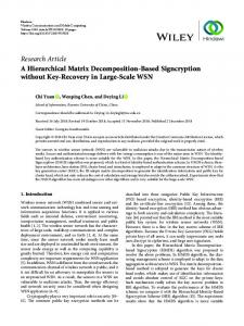
After selecting 𝐽𝑘 in (7), an extra block column 𝐽̄𝑘 with 𝐽̄𝑘 ∩ 𝐽𝑘 = ∅ is selected by repeating (7) with 𝐸𝑘−1 (𝐼𝑘 , 𝐽𝑘𝖼 ) for use in the next iteration. See Fig. 1a for an illustration of the procedure. • Form the low-rank product 𝑈𝑘 𝑉𝑘 . Let 𝐶𝑘 = 𝐸𝑘−1 (∶, 𝐽𝑘 ), 𝑅𝑘 = 𝐸𝑘−1 (𝐼𝑘 , ∶) and 𝑊𝑘 = 𝐸𝑘−1 (𝐼𝑘 , 𝐽𝑘 ), 𝐸𝑘−1 can be approximated by an ID-type decomposition 𝐸𝑘−1 ≈ 𝐶𝑘 𝑊𝑘† 𝑅𝑘 = 𝑈𝑘 𝑉𝑘 3 . The pseudo inverse is computed via rank-revealing QR as follows (i.e., the LRID algorithm at line 11). Note that the effective rank increase is 𝑑𝑘 ≤ 𝑑.

[𝑄, 𝑇 , 𝐽 , 𝑑𝑘 ] = 𝚀𝚁(𝑊𝑘 , 𝜖) 𝑈𝑘 = 𝐶𝑘 (∶, 𝐽 ), 𝑉𝑘 = 𝑇

−1

𝑡

𝑄 𝑅𝑘

(8) (9)

4

Yang Liu ET AL

Algorithm 2: Blocked adaptive cross approximation algorithm (BACA) input : Matrix 𝐴 ∈ ℝ𝑚×𝑛 , block size 𝑑, relative tolerance 𝜖 output: Low-rank approximation of 𝐴 ≈ 𝑈 𝑉 with rank 𝑟 1 𝑈 = 0, 𝑉 = 0, 𝑟 = 0, 𝜇 = 0, 𝐽̄0 is a random index set of cardinality 𝑑; 2 for 𝑘 = 1 to (𝑚 + 𝑛)∕𝑑 do 3 𝐶̄𝑘 = 𝐴(∶, 𝐽̄𝑘−1 ) − 𝑈 𝑉 (∶, 𝐽̄𝑘−1 ); 4 [𝑄𝑐𝑘 , 𝑇𝑘𝑐 , 𝐼𝑘 ] = QR(𝐶̄𝑘𝑡 , 𝑑); 5 𝑅𝑘 = 𝐴(𝐼𝑘 , ∶) − 𝑈 (𝐼𝑘 , ∶)𝑉 ; 6 [𝑄𝑟𝑘 , 𝑇𝑘𝑟 , 𝐽𝑘 ] = QR(𝑅𝑘 , 𝑑); 7 𝐶𝑘 = 𝐴(∶, 𝐽𝑘 ) − 𝑈 𝑉 (∶, 𝐽𝑘 ); 8 𝑊𝑘 = 𝐴(𝐼𝑘 , 𝐽𝑘 ) − 𝑈 (𝐼𝑘 , ∶)𝑉 (∶, 𝐽𝑘 ); 9 𝑅̄ 𝑘 (∶, 𝑗) = 𝑅𝑘 (∶, 𝑗) for 𝑗 ∉ 𝐽𝑘 and zero elsewhere; 10 [𝑄̄ 𝑟𝑘 , 𝑇̄𝑘𝑟 , 𝐽̄𝑘 ] = QR(𝑅̄ 𝑘 , 𝑑); 11 [𝑈𝑘 , 𝑉𝑘 , 𝑑𝑘 ] = LRID(𝐶𝑘 , 𝑊𝑘 , 𝑅𝑘 ); 12 𝑟𝑘 ← 𝑟𝑘 + 𝑑𝑘 ; 13 𝜈 = LRnorm(𝑈𝑘 , 𝑉𝑘 ); 14 𝜇 ← LRnormUp(𝑈 , 𝑉 , 𝜇, 𝑈𝑘 , 𝑉𝑘 , 𝜈); 15 𝑈 ← [𝑈 , 𝑈𝑘 ], 𝑉 ← [𝑉 ; 𝑉𝑘 ]; 16 Terminate if 𝜈 < 𝜖𝜇. 17

18 19 20 21 22

23 24 25 26

27 28

Function LRID (𝐶,𝑊 ,𝑅,𝜖) input : 𝐶 = 𝐴(∶, 𝐽 ), 𝑅 = 𝐴(𝐼, ∶), 𝑊 = 𝐴(𝐼, 𝐽 ) with 𝐼, 𝐽 of same cardinality output: 𝐴 = 𝑈 𝑉 with 𝑈 ∈ ℝ𝑚×𝑟 , 𝑉 ∈ ℝ𝑟×𝑛 [𝑄, 𝑇 , 𝐽̄, 𝑟] = QR(𝑊 , 𝜖); 𝑈 = 𝐶(∶, 𝐽̄); 𝑉 = 𝑇 −1 𝑄𝑡 𝑅; return 𝑈 , 𝑉 , 𝑟 Function LRnorm (𝑈 ,𝑉 ) input : 𝐴 = 𝑈 𝑉 output: ‖𝐴‖𝐹 [𝑄1 , 𝑇1 ] = QR(𝑈 ); [𝑄2 , 𝑇2 ] = QR(𝑉 𝑡 ); ‖ ‖ return ‖𝑇1 𝑇2𝑡 ‖ ; ‖ ‖𝐹 Function LRnormUp (𝑈 , 𝑉 , 𝜈, 𝑈𝑘 , 𝑉𝑘 , 𝜈) ̄ ̄ ̄‖ input : 𝑈 ∈ ℝ𝑚×𝑟 , 𝑉 ∈ ℝ𝑟×𝑛 , 𝑈̄ ∈ ℝ𝑚×̄𝑟 , 𝑉̄ ∈ ℝ𝑟̄×𝑛 , 𝜈 = ‖𝑈 𝑉 ‖𝐹 , 𝜈̄ = ‖ ‖𝑈 𝑉 ‖𝐹 ̄ output: ‖ ; 𝑉̄ ]‖ ‖[𝑈 , 𝑈∑][𝑉 ‖𝐹 𝑟 ∑𝑟̄ 2 2 𝑠 = 𝜈 + 𝜈̄ + 𝑖=1 𝑗=1 2𝑉 (𝑖, ∶)𝑉̄ 𝑡 (𝑗, ∶)𝑈̄ 𝑡 (∶, 𝑗)𝑈 (∶, 𝑖); √ return 𝑠

‖ • Compute 𝜈 = ‖ ‖𝑈𝑘 𝑉𝑘 ‖𝐹 and update 𝜇 = ‖𝑈 𝑉 ‖𝐹 . Assuming constant block size 𝑑, the norm of the low-rank update can be computed in 𝑂(𝑛𝑑𝑘2 ) operations (line 13) via [𝑄𝑈𝑘 , 𝑇𝑈𝑘 ] = 𝚀𝚁(𝑈𝑘 ), [𝑄𝑉𝑘 , 𝑇𝑉𝑘 ] = 𝚀𝚁(𝑉𝑘𝑡 ) ‖ ‖ 𝜈 = ‖𝑇𝑈𝑘 𝑇𝑉𝑡 ‖ 𝑘 ‖𝐹 ‖ Once 𝜈 is computed, the norm of 𝑈 𝑉 can be updated efficiently in 𝑂(𝑛𝑟𝑘 𝑑𝑘 ) operations (line 14) as 𝜇2 ← 𝜇2 + 𝜈 2 +

𝑟𝑘 𝑑 𝑘 ∑ ∑ 𝑖=1 𝑗=1

2𝑉 (𝑖, ∶)𝑉𝑘 𝑡 (𝑗, ∶)𝑈𝑘 𝑡 (∶, 𝑗)𝑈 (∶, 𝑖)

(10) (11)

(12)

5

Yang Liu ET AL

Ut1n1 St1n1Vt1n1

Jk Ck

J k -1 J k

I k Rk

Ut1n 2 St1n 2Vt1n 2 Combine

Vk = T -1Q t Rk

Kk

Ut 2n1 St 2n1Vt 2n1

SVD

Ut 2n 2 St 2n 2Vt 2n 2

U k = Ck (:, J ) Utn Stn Vtn

Ut1n St1n Vt1n Combine (a)

SVD

Ut 2n St 2n Vt 2n (b)

FIGURE 1 (a) Selection of 𝐼𝑘 /𝐽𝑘 and form the low-rank update 𝑈𝑘 𝑉𝑘 . (b) Low-rank merge operation where 𝑟𝑘 represents the column dimension of 𝑈 at iteration 𝑘. Then the algorithm updates 𝑈 , 𝑉 as [𝑈 , 𝑈𝑘 ], [𝑉 ; 𝑉𝑘 ] and tests the stopping criteria 𝜈 < 𝜖𝜇. It is worth mentioning that the choice of 𝑑 depends on the tradeoff between efficiency and robustness of the BACA algorithm. When 𝑑 < 𝑟, the algorithm requires 𝑂(𝑛𝑟2 ) operations assuming convergence in 𝑂(𝑟∕𝑑) iterations as each iteration requires 𝑂(𝑛𝑟𝑘 𝑑) operations. For example, BACA reduces to ACA when 𝑑 = 1 except for a slightly different strategy for selecting pivot rows and columns. On the other hand, BACA converges in a constant number of iterations when 𝑑 ≫ 𝑟. For example, BACA reduces to QRCP-based ID when 𝑑 = min{𝑚, 𝑛} (note that only line 11 is executed). In this case the algorithm requires 𝑂(𝑛2 𝑟) operations but enjoys the provable convergence of QRCP. The BACA algorithm oftentimes exhibits overestimated ranks compared to those revealed by truncated SVD. Therefore, a SVD re-compression of 𝑈 and 𝑉 may be needed via first computing a QR of 𝑈 and 𝑉 as [𝑄𝑈 , 𝑇𝑈 ] = 𝚀𝚁(𝑈 ), [𝑄𝑉 , 𝑇𝑉 ] = 𝚀𝚁(𝑉 𝑡 ), and then truncated a SVD of 𝑇𝑈 𝑇𝑉𝑡 15 . The results can be viewed as a truncated SVD of 𝐴 and we assume this is the output of the BACA algorithm in the rest of this paper.

Algorithm 3: Hierarchical low-rank merge algorithm with BACA (H-BACA) input : Matrix 𝐴 ∈ ℝ𝑚×𝑛 , number of leaf-level subblocks 𝑛𝑏 , block size 𝑑 of leaf-level BACA, relative tolerance 𝜖 output: Low-rank approximation of 𝐴 ≈ 𝑈 𝑉 with rank 𝑟 1 Create 𝐿-level trees on index vectors [1, 𝑚] and [1, 𝑛] with index set 𝐼𝜏 and 𝐽𝜈 for nodes 𝜏 and 𝜈 at each level, √ 𝐿 = log2 𝑛𝑏 , the leaf and root levels are denoted 0 and 𝐿, respectively; 2 for 𝑙 = 0 to 𝐿 do 3 foreach 𝐴𝜏𝜈 = 𝐴(𝐼𝜏 , 𝐽𝜈 ) at level 𝑙 do 4 if leaf-level then 5 [𝑈𝜏𝜈 , Σ𝜏𝜈 , 𝑉𝜏𝜈 , 𝑟𝜏𝜈 ] = BACA(𝐴𝜏𝜈 , 𝑑, 𝜖); 6 7 8 9 10 11 12 13 14 15 16

else Let 𝜏1 , 𝜏2 and 𝜈1 , 𝜈2 denote children of 𝜏 and 𝜈; for 𝑖 = 1 to 2 do 𝑈̄ 𝜏𝑖 𝜈 = [𝑈𝜏𝑖 𝜈1 Σ𝜏𝑖 𝜈1 , 𝑈𝜏𝑖 𝜈2 Σ𝜏𝑖 𝜈2 ]; 𝑉̄𝜏𝑖 𝜈 = diag(𝑉𝜏𝑖 𝜈1 , 𝑉𝜏𝑖 𝜈2 ); [𝑈𝜏𝑖 𝜈 , Σ𝜏𝑖 𝜈 , 𝑉𝜏𝑖 𝜈 , 𝑟𝜏𝑖 𝜈 ] ← SVD(𝑈̄ 𝜏𝑖 𝜈 , 𝜖); 𝑉𝜏𝑖 𝜈 ← 𝑉𝜏𝑖 𝜈 𝑉̄𝜏𝑖 𝜈 ; 𝑈̄ 𝜏𝜈 = diag(𝑈𝜏𝑖 𝜈 , 𝑈𝜏𝑖 𝜈 ); 𝑉̄𝜏𝜈 = [Σ𝜏 𝜈 𝑉𝜏 𝜈 ; Σ𝜏 𝜈 𝑉𝜏 𝜈 ]; 1

1

2

2

[𝑈𝜏𝜈 , Σ𝜏𝜈 , 𝑉𝜏𝜈 , 𝑟𝜏𝜈 ] ← SVD(𝑉̄𝜏𝜈 , 𝜖); 𝑈𝜏𝜈 ← 𝑈̄ 𝜏𝜈 𝑈𝜏𝜈 ;

6

Yang Liu ET AL

0 0 2 2 4 4

3 3

0 0 2 2

5 5

4 4

1 1

6 6 7 7 l =0

1 1 3 3

0 0 2 2

5 5

4 4

6 6 7 7 l = 0.5

1 1 3 3

0 2

0

1

3

0 1 2 3

2

3

0 1 2 3

5 5

4

5

4 5

4

5

4 5

6 6 7 7 l =1

6

7 6 7 l = 1.5

6

7 6 7 l =2

1

FIGURE 2 Parallel hierarchical merge with 8 processes

3.3

Hierarchical Low-Rank Merge

The proposed BACA algorithm can be further enhanced with a hierarchical low-rank merge algorithm to achieve improved robustness and parallelism. The low-rank merge operation resembles arithmetics for Hierarchical matrices 16 . Given a matrix 𝐴 ∈ ℝ𝑚×𝑛 with 𝑚 ≈ 𝑛, the algorithm first creates 𝐿-level binary trees for index vectors [1, 𝑚] and [1, 𝑛] with index set 𝐼𝜏 and 𝐽𝜈 for nodes 𝜏 and 𝜈 at each level. This process generates 𝑛𝑏 leaf-level submatrices. We denote submatrices associated with 𝜏, 𝜈 as 𝐴𝜏𝜈 = 𝐴(𝐼𝜏 , 𝐽𝜈 ) and their truncated SVD as [𝑈𝜏𝜈 , Σ𝜏𝜈 , 𝑉𝜏𝜈 , 𝑟𝜏𝜈 ] = 𝚂𝚅𝙳(𝐴𝜏𝜈 , 𝜖). Here 𝑟𝜏𝜈 is the 𝜖-rank of 𝐴𝜏𝜈 . We begin with low-rank decompositions of leaf-level submatrices 𝐴𝜏𝜈 computed via BACA and pair-wise re-compress them via rankrevealing decompositions until we reach the root level. Here, we deploy truncated SVD as the re-compression tool but other tools such as ID, QR, UTV and their randomized variants can also be applied. Fig. 1b illustrates one re-compression operation for transforming SVDs of 𝐴𝜏𝑖 𝜈𝑗 , 𝑖 = 1, 2, 𝑗 = 1, 2 into that of 𝐴𝜏𝜈 , where 𝜏𝑖 and 𝜈𝑗 are children of 𝜏 and 𝜈, respectively. The operation first column-wise compresses 𝐴𝜏𝑖 𝜈𝑗 , 𝑖 = 1, 2, 𝑗 = 1, 2 and then row-wise compresses the results 𝐴𝜏𝑖 𝜈 , 𝑖 = 1, 2. Specifically, the column-wise compression step is composed of one concatenation operation in (13) and one compression operation in (14): 𝑈̄ 𝜏𝑖 𝜈 = [𝑈𝜏𝑖 𝜈1 Σ𝜏𝑖 𝜈1 , 𝑈𝜏𝑖 𝜈2 Σ𝜏𝑖 𝜈2 ], 𝑉̄𝜏𝑖 𝜈 = diag(𝑉𝜏𝑖 𝜈1 , 𝑉𝜏𝑖 𝜈2 ) [𝑈𝜏 𝜈 , Σ𝜏 𝜈 , 𝑉𝜏 𝜈 , 𝑟𝜏 𝜈 ] ← 𝚂𝚅𝙳(𝑈̄ 𝜏 𝜈 , 𝜖), 𝑉𝜏 𝜈 ← 𝑉𝜏 𝜈 𝑉̄𝜏 𝜈 𝑖

𝑖

𝑖

𝑖

𝑖

𝑖

𝑖

𝑖

(13) (14)

with 𝑖 = 1, 2. Let 𝐴̄ 𝜏𝑖 𝜈 = 𝑈̄ 𝜏𝑖 𝜈 𝑉̄𝜏𝑖 𝜈 denote the submatrix before the SVD truncation. Similarly, the row-wise compression step can be performed via column-wise merge of 𝐴𝑡𝜏 𝜈 , 𝑖 = 1, 2. Note the algorithm returns a truncated SVD after 𝐿 steps. The 𝑖 above-described hierarchical algorithm, when combined with BACA, is dubbed H-BACA (Algorithm 3). In the following, a distributed-memory implementation of the H-BACA algorithm is described. Without loss of generality, √ √ it is assumed 𝑚 = 𝑛 = 2𝑖 . The proposed parallel implementation first creates approximately log 𝑝-level binary trees of 𝑝 row and column processes with 𝑝 denoting the total number of MPI processes. One process performs BACA compression of at least one leaf-level submatrix and low-rank merge operations from the bottom up until it reaches a submatrix shared by more than one process. Then, all such blocks are handled by ScaLAPACK with process grids that aggregate those in corresponding submatrices. As an example, the parallel H-BACA algorithm with process count 𝑝 = 8 and level count of the hierarchical merge 𝐿 = 2 are illustrated in Fig. 2. The workload of each process is labeled with its process rank and highlighted with one color. The solid lines show the partitioning of the submatrices at each level and the dashed lines represent the ScaLAPACK submatrix tiles. First, merge operations at 𝑙 = 0, 0.5 are handled locally by one process without any communication. Next, merge operations at 𝑙 = 1, 1.5, 2 are handled by ScaLAPACK grids of 2 × 1, 2 × 2, and 4 × 2, respectively. For simplicity, we select the tile size in ScaLAPACK as 𝑛0 × 𝑛0 where 𝑛0 is the dimension of the finest-level submatrices in the hierarchical merge algorithm. In this case, the only required data redistribution is from step 𝑙 = 1 to 𝑙 = 1.5. However, the tile size may be set to much smaller numbers in practice requiring data redistribution at each row/column re-compression step.

4 4.1

PERFORMANCE ANALYSIS Error analysis

First, we provide a simple error analysis for Algorithm 3. Let 𝐴′𝜏𝜈 = 𝑈𝜏𝜈 Σ𝜏𝜈 𝑉𝜏𝜈 , we would like to provide an error bound for ‖𝐴𝜏𝜈 − 𝐴′ ‖ when 𝜏, 𝜈 represent the root nodes of the trees. Despite the lack of analysis for the BACA algorithm for general ‖ 𝜏𝜈 ‖𝐹 ′ ‖ matrices, we assume that the BACA algorithm for leaf-level submatrices attains the desired accuracy ‖ ‖𝐴𝜏𝜈 − 𝐴𝜏𝜈 ‖2 ≤ 𝜖, 𝜏, 𝜈 are leaf-level nodes. Note that this holds true when block size 𝑑 is sufficiently large (BACA can achieve the same accuracy as QRCP when 𝑑 = 𝑛). We first provide an error bound for the low-rank merge operation. As the merge process consists of 𝐿

7

Yang Liu ET AL

𝑑 = 𝑂(1) √ 𝑑 = 𝑂(𝑛∕ 𝑛𝑏 )

constant rank 𝑟𝑙 = 𝑟 √ 𝑂(𝑟2 𝑛 𝑛𝑏 ) 𝑂(𝑟𝑛2 )

increasing rank √ 𝑟𝑙 = 𝑟∕ 𝑛𝑏 × 2𝑙 𝑂(𝑟2 𝑛) √ 𝑂(𝑟𝑛2 ∕ 𝑛𝑏 + 𝑟2 𝑛)

FIGURE 2 Flop counts for algorithm 3

1

steps, step 𝑙 performs column-wise re-compression and step 𝑙 + 21 performs row-wise re-compression. Let 𝐴𝑙 and 𝐴𝑙+ 2 denote the matrices concatenated by all submatrices before the step 𝑙 and 𝑙 + 12 re-compression, 𝑙 = 1, 2, ..., 𝐿. Note that 𝐴0 = 𝐴, 𝐴1 denotes the matrix after the leaf-level BACA compression, and 𝐴𝐿+1 denotes the final matrix attained by the H-BACA ‖ ‖ ‖ ‖ algorithm. For the column-wise re-compression step at (14), we have ‖𝑈𝜏𝑖 𝜈 Σ𝜏𝑖 𝜈 𝑉𝜏𝑖 𝜈 − 𝑈̄ 𝜏𝑖 𝜈 ‖ ≤ 𝜖 ‖𝑈̄ 𝜏𝑖 𝜈 ‖ from SVD and hence ‖ ‖2 ‖ ‖2 1 ‖̄ ‖ ‖ ‖ ‖𝐴𝜏𝑖 𝜈 − 𝐴′𝜏𝑖 𝜈 ‖ ≤ 𝜖 ‖𝐴̄ 𝜏𝑖 𝜈 ‖ with 𝐴̄ 𝜏𝑖 𝜈 = 𝑈̄ 𝜏𝑖 𝜈 𝑉̄𝜏𝑖 𝜈 due to orthonormality of 𝑉̄𝜏𝑖 𝜈 in (13). For the whole matrix 𝐴𝑙+ 2 , ‖ ‖2 ‖ ‖2 1 2 1‖ 𝑙 1 ∑‖ ̄ ‖2 ‖ (15) ‖𝐴𝜏𝑖 𝜈 − 𝐴′𝜏𝑖 ,𝜈 ‖ ≤ ‖𝐴 − 𝐴𝑙+ 2 ‖ = ‖𝐹 ‖𝐹 𝑟𝑙 ‖ 𝑟𝑙 𝜏,𝜈,𝑖 ‖ ∑‖ ∑‖ ‖2 ‖2 (16) ‖𝐴̄ 𝜏𝑖 𝜈 − 𝐴′𝜏𝑖 𝜈 ‖ ≤ 𝜖 2 ‖𝐴̄ 𝜏𝑖 𝜈 ‖ ‖ ‖2 ‖ ‖2 𝜏,𝜈,𝑖 𝜏,𝜈,𝑖 ∑‖ ‖2 ‖ ‖2 ≤ 𝜖2 (17) ‖𝐴̄ 𝜏𝑖 𝜈 ‖ = 𝜖 2 ‖𝐴𝑙 ‖ ≤ 𝜖 2 ‖𝐴‖2𝐹 ‖ ‖𝐹 ‖ ‖𝐹 𝜏,𝜈,𝑖

Here, 𝑟𝑙 represents the maximum rank revealed at steps 𝑙 and 𝑙 + 21 . The last inequality holds true due to the property that SVD 1 2 ‖ ‖ truncation does not increase the Frobenius norm. Similarly it can be shown that for step 𝑙+ 12 , 𝑟1 ‖𝐴𝑙+1 − 𝐴𝑙+ 2 ‖ ≤ 𝜖 2 ‖𝐴‖2𝐹 ; and ‖𝐹 ‖ 𝑙 1 ‖2 ≤ 𝜖 2 ‖𝐴‖2 . Therefore we attain the following error bound for the H-BACA algorithm: for the initial BACA step, 𝑟1 ‖ 𝐴 − 𝐴 ‖ ‖𝐹 𝐹 𝑙 ‖ 𝐿+1 ‖ ‖ ‖ − 𝐴‖ ≤ ‖𝐴1 − 𝐴‖ (18) ‖𝐴 ‖ ‖𝐹 ‖ ‖𝐹 𝐿 𝐿 ∑ ∑ 1 1 ‖ 𝑙 ‖ ‖ ‖ 𝑙+1 + (19) ‖𝐴 − 𝐴𝑙+ 2 ‖ + ‖𝐴 − 𝐴𝑙+ 2 ‖ ‖ ‖𝐹 ‖𝐹 ‖ 𝑙=1 𝑙=1 √ ≤ 𝜖(2𝐿 + 1) 𝑟 ‖𝐴‖𝐹 (20) Note that the factor (2𝐿 + 1) in (20) represents an error upper bound. From our numerical results the error shows only weak dependence on the number of levels 𝐿.

4.2

Computational costs

Next, the computational costs of the H-BACA algorithm is analyzed. Let 𝑟𝑙 denote the maximum rank revealed at level 𝑙, 𝑙 = 0, 1, .., 𝐿. The costs are analyzed for two cases of rank distributions, i.e., 𝑟𝑙 = 𝑟 (ranks stay constant during the merge) and √ 𝑟𝑙 = 2𝑙 𝑟∕ 𝑛𝑏 (rank increases by a factor of 2 per level). The constant-rank case is often valid for matrices with their numerical rank independent of matrix dimensions; the increasing-rank case holds true for matrices (e.g., those arising from high-frequency wave equations) whose rank is a constant proportion of the matrix dimensions. Recall that for the leaf-level BACA compressions, the computational costs 𝑐𝑖 are: 𝑛 𝑐𝑖 = √ 𝑟20 𝑛𝑏 , if 𝑑 = 𝑂(1) (21) 𝑛𝑏 ) ( √ 𝑛 2 𝑟0 𝑛𝑏 , if 𝑑 = 𝑂(𝑛∕ 𝑛𝑏 ) (22) 𝑐𝑖 = √ 𝑛𝑏 √ which represent the complexity with ACA and QRCP when 𝑑 = 1 and 𝑑 = 𝑛∕ 𝑛𝑏 , respectively.

8

Yang Liu ET AL

√ Let 𝑛𝑙 = 2𝑙 𝑛∕ 𝑛𝑏 denote the size of submatrices 𝐴𝜏,𝜈 at level 𝑙. The computational costs 𝑐𝑚 of hierarchical merge operations can be estimated as 𝐿 ∑ 4𝐿−𝑙 𝑛𝑙 𝑟2𝑙 (23) 𝑐𝑚 = 𝑙=1

Summing up (21)-(23) for the two cases of rank distributions, the overall costs of the H-BACA algorithm are summarized in √ Table 1. Not surprisingly, the hierarchical merge algorithm induces a computational overhead of 𝑛𝑏 when 𝑑 = 𝑂(1) and ranks √ √ stay constant; it also permits a reduction of computation time by a factor 𝑛𝑏 when 𝑑 = 𝑂(𝑛∕ 𝑛𝑏 ) and ranks increase. For other cases in Table 1, the complexity scales like the BACA algorithm.

5

NUMERICAL RESULTS

This section presents several numerical results to demonstrate the accuracy and efficiency of the proposed H-BACA algorithm. 2 −‖𝑥𝑖 −𝑥𝑗 ‖ The matrices in all numerical examples are generated from the following kernels: 1. Gaussian kernel: 𝐴𝑖,𝑗 = exp( 2ℎ ), 2 8×1 784×1 𝑖, 𝑗 = 1, ..., 2𝑛. Here ℎ is the Gaussian width, and 𝑥𝑖 , 𝑥𝑗 ∈ ℝ and ℝ are feature vectors in one subset of the SUSY and MNIST Data Sets from the UCI Machine Learning Repository 20 , respectively. Note that the Gaussian kernel permits low-rank ‖ ‖ compression as shown in 21–23 2. Helmholtz kernel: 𝐴𝑖,𝑗 = 𝐻0(2) (𝑘 ‖𝑥𝑖 − 𝑥𝑗 ‖). Here 𝐻0(2) is the second kind Hankel function of ‖ ‖ order 0, 𝑘 is the free-space wavenumber, 𝑥𝑖 , 𝑥𝑗 ∈ ℝ2×1 are discretization points (15 points per wavelength) of two 2-D parallel strips of length 1 and distance 1. Note that 𝐴 is a complex-valued matrix. 3. Polynomial kernel: 𝐴𝑖,𝑗 = (𝑥𝑡𝑖 𝑥𝑗 + ℎ)2 . Here 𝑥𝑖 , 𝑥𝑗 ∈ ℝ50×1 are points from a randomly generated dataset, and ℎ is a regularization parameter. 4. ToeplitzQchem kernel: (𝑖−𝑗) √ . Throughout this section, we refer to ACA and QRCP as special cases of BACA when 𝑑 = 1 and 𝑑 = 𝑛∕ 𝑛𝑏 , 𝐴𝑖,𝑗 = (−1) (𝑖−𝑗)2 respectively. In all examples, the algorithm is applied to the offdiagonal submatrix 𝐴(1 ∶ 𝑛, 1 + 𝑛 ∶ 2𝑛) assuming rows/columns of 𝐴 have been properly permuted. All experiments are performed on the Cori Haswell machine at NERSC, which is a Cray XC40 system and consists of 2388 dual-socket nodes with Intel Xeon E5-2698v3 processors running 16 cores per socket. The nodes are configured with 128 GB of DDR4 memory at 2133 MHz.

5.1

Convergence

First, the convergence of the proposed BACA algorithm is investigated using multiple matrices: Gaussian-SUSY matrices with 𝑛 = 5000, ℎ = 1.0, 0.2, Polynomial matrices with 𝑛 = 10000, ℎ = 0.2, and Helmholtz matrices with 𝑛 = 20000. The corresponding 𝜖-ranks are 𝑟 = 4683, 1723, 1293, 302 for 𝜖 = 1𝑒−6 . The convergence histories of BACA with 𝑑 = 1, 32, 64, 128, 256 ‖ and 𝑛 are plotted in Fig. 3. The residual error for 𝑑 < 𝑛 is defined as ‖ ‖𝑈𝑘 𝑉𝑘 ‖𝐹 ∕ ‖𝑈 𝑉 ‖𝐹 from (11). For 𝑑 = 1, 32, 64, 128, 256, the iteration number is multiplied with 𝑑 for 𝑑 < 𝑛 to reflect the true convergence performance, as BACA picks 𝑑 columns/rows per iteration. For 𝑑 = 𝑛, the convergence history of QRCP in LRID is plotted. The residual error for QRCP is defined as 𝑇 (𝑘, 𝑘)∕𝑇 (1, 1) with [𝑄, 𝑇 , 𝐽 ] = 𝚀𝚁(𝐴, 𝜖). For the Gaussian-SUSY matrices, the baseline ACA algorithm (𝑑 = 1) behaves poorly with smaller ℎ due to faster exponential decay of the Gaussian kernel. In fact, the residual exhibits wild oscillations and even causes early iteration termination for ℎ = 0.2 (see Fig. 3b). The QRCP algorithm (𝑑 = 𝑛), in stark contrast, achieves the desired accuracy after approximately 𝑟 iterations (although requiring the 𝑂(𝑛2 ) operations per iteration). The proposed BACA algorithm (𝑑 = 32, 64, 128, 256) shows increasingly smooth residual histories as 𝑑 increases. For the Polynomial (Fig. 3c) and Helmholtz (Fig. 3d) matrices, BACA also shows better convergence behaviors compared to ACA with even small block sizes 𝑑 > 1.

5.2

Accuracy

Next, the accuracy of the H-BACA algorithm is demonstrated using the following matrices: two Gaussian-SUSY matrices with 𝑛 = 5000, ℎ = 1.0, 0.2, one Polynomial matrix with 𝑛 = 10000, ℎ = 0.2 and one Helmholtz matrices with 𝑛 = 5000. The relative Frobenious-norm error ‖𝐴 − 𝑈 𝑉 ‖𝐹 ∕ ‖𝐴‖𝐹 is computed via changing number of leaf-level submatrices 𝑛𝑏 and block size 𝑑. When ℎ = 1.0 for the Gaussian-SUSY matrix (Fig. 4a), the H-BACA algorithms achieve desired accuracies √ (𝜖 = 1𝑒−2 , 1𝑒−6 , 1𝑒−10 ) using the baseline ACA (𝑑 = 1), BACA (𝑑 = 32), QRCP (𝑑 = 𝑛∕ 𝑛𝑏 ) when 𝑛𝑏 = 1 and the hierarchical merge operation only causes slight error increases compared to error estimate (20) as 𝑛𝑏 increases. Similar results have been

9

Yang Liu ET AL

residual

10

0

10

-2

10

-4

10

-6

0

500

1000

1500

2000

2500

3000

3500

iteration count (b) Gaussian-SUSY( (ℎ = 0.2)

(a) Gaussian-SUSY (ℎ = 1.0)

0

10

-2

10

-4

10

-6

10

residual

residual

10

0

200

400

600

800

1000

iteration count (c) Polynomial

1200

1400

1600

0

10

-2

10

-4

10

-6

0

200

400

600

800

1000

iteration count (d) Helmholtz

FIGURE 3 Convergence history of BACA for the Gaussian kernel with (a) Gaussian-SUSY with ℎ = 1.0, (b) Gaussian-SUSY with ℎ = 0.2, (c) Polynomial and (d) Helmholtz matrices

observed for the Polynomial (Fig. 4c) and Helmholtz (Fig. 4d) matrices. When ℎ = 0.2 for the Gaussian-SUSY matrix (Fig. 4b), H-BACA with QRCP still attains desired accuracy for all data points while H-BACA with ACA fails. In comparison, the H-BACA with 𝑑 = 32 is slightly better than 𝑑 = 1 when 𝑛𝑏 = 1 but dramatically improves as 𝑛𝑏 increases.

5.3

Efficiency

This subsection provides several examples to verify the complexity estimates in Table 1. H-BACA with leaf-level ACA (𝑑 = 1), √ BACA (𝑑 = 8, 16, 32, 64, 128, 256), and QRCP (𝑑 = 𝑛∕ 𝑛𝑏 ) is tested for the following matrices: one Helmholtz matrix with 𝑛 = 40000, 𝜖 = 1𝑒−4 , one Gaussian-SUSY matrix with 𝑛 = 5000, ℎ = 1.0, 𝜖 = 1𝑒−2 , one Gaussian-MNIST matrix with 𝑛 = 5000, ℎ = 3.0, 𝜖 = 1𝑒−2 , one polynomial matrix with 𝑛 = 2500, ℎ = 0.2, 𝜖 = 1𝑒−4 , and one ToeplitzQchem matrix with 𝑛 = 100000, 𝜖 = 1𝑒−4 . The corresponding 𝜖-ranks are 292, 259, 137, 199 and 9, respectively. The computational times are measured and plotted in Fig. 5. Note that the data points where the algorithm fails are marked with solid triangles. For the algorithm with QRCP, Table 1 suggests that the CPU time stays constant w.r.t 𝑛𝑏 when the hierarchical merge operation attains √ constant ranks 𝑟𝑙 , which is partially observed for Gaussian and ToeplitzQchem matrices. Also, the factor of 1∕ 𝑛𝑏 reduction in CPU time when 𝑟𝑙 increases is also observed for the Helmholtz matrix. For the algorithm with ACA and BACA, Table I predicts √ increasing (with a factor of 𝑛𝑏 ) and constant time when 𝑟𝑙 stays constant and increases, respectively. We observe increasing CPU time w.r.t. 𝑛𝑏 for all matrices when 𝑛𝑏 is large, but non-increasing CPU time when 𝑛𝑏 is small. Note that when 𝑛𝑏 is changed from 1 to 16, the CPU time is even reduced due to improved BLAS performance. In addition, we observe reduced CPU time as the block size 𝑑 increases for most examples due to better convergence and BLAS performance. However, when 𝑛𝑏 is large and/or the 𝜖-rank of 𝐴 is small, large 𝑑 slows down BACA due to overestimation of ranks of corresponding (sub)matrices.

5.4

Parallel performance

Finally, the parallel performance of the H-BACA algorithm is demonstrated via a strong scaling study with the Helmholtz matrices. Here 𝑛 = 160000 and the wavenumbers are chosen such that the 𝜖-ranks with 𝜖 = 1𝑒−4 are 𝑟 = 30, 450 and 890,

10

Yang Liu ET AL 0

10

-2

10

-4

10

-6

10

10

0

10

10-2

Error

10

10

-4

10

-6

10

-8

-8

-10

10

1

4

16

64

256

-10

1

1024

4

(a) Gaussian-SUSY (ℎ = 1.0)

0

10

10 10

-2

10

-4

10

-6

10

-8

10

-10

10

-12

10

-14

4

16 (c) Polynomial

64

64

256

1024

256

1024

256

1024

0

10

-2

10

-4

10

-6

10

-8

10 1

16

(b) Gaussian-SUSY (ℎ = 0.2)

-10

1

4

16

64

(d) Helmholtz

FIGURE 4 Measured error of H-BACA for the (a) Gaussian-SUSY with ℎ = 1.0, (b) Gaussian-SUSY with ℎ = 0.2, (c) Polynomial and (d) Helmholtz matrices.

respectively. H-BACA with 𝑑 = 1 is tested with process count 𝑝 = 4, ..., 1024. The ScaLAPCK tile size is set to 64×64. For small rank 𝑟 = 30, poor parallel efficiency is due to partially utilized process grids at each re-compression step and the computational √ overhead of 𝑛𝑏 ; for larger rank 𝑟 = 450, 890, good parallel efficiencies are achieved (see Fig. 5d). Not surprisingly, the parallel runtime is dominated by that of ScaLAPACK and redistributions between each re-compression step.

6

CONCLUSION

This paper presents a fast and robust low-rank matrix decomposition algorithm given that any matrix entry can be evaluated in 𝑂(1) time. The proposed algorithm performs blocked adaptive cross approximation (BACA) algorithms on submatrices followed by a hierarchical low-rank merge algorithm. The BACA algorithm significantly improves the robustness of the baseline ACA algorithm and maintains low computational complexity. The H-BACA algorithm combines results of BACA into the desired low-rank decomposition to further increase robustness and parallelism. Analysis and numerical examples demonstrate favorable efficiency and accuracy of the proposed algorithm for broad ranges of matrices.

ACKNOWLEDGMENT This research was supported in part by the Exascale Computing Project (17-SC-20-SC), a collaborative effort of the U.S. Department of Energy Office of Science and the National Nuclear Security Administration, and in part by the U.S. Department of Energy, Office of Science, Office of Advanced Scientific Computing Research, Scientific Discovery through Advanced Computing (SciDAC) program through the FASTMath Institute under Contract No. DE-AC02-05CH11231 at Lawrence Berkeley National Laboratory. This research used resources of the National Energy Research Scientific Computing Center (NERSC), a U.S. Department of Energy Office of Science User Facility operated under Contract No. DE-AC02-05CH11231.

11

Yang Liu ET AL

10

10

2

1

1

4

16

64

256

10

3

10

2

10

1

10

0

1

1024

4

16

(a) Helmholtz

10

2

10

1

256

1024

64

256

1024

(b) Gaussian-SUSY

10

10

64

1

0

1

4

16

64

256

1024

1

4

16 (d) Polynomial

(c) Gaussian-MNIST

103 r890 r450 r30

10

2

Time

102

10

1

10

0

101

100 1

4

16

64

256

1024

4

8

16

32

64

128

256

512

1024

p (e) ToeplitzQchem

(f) Helmholtz

FIGURE 5 CPU time of H-BACA for (a) Helmholtz, (b) Gaussian-SUSY, (c) Gaussian-MNIST, (d) Polynomial, (e) ToeplitzQchem matrices with varying 𝑛𝑏 . (f) CPU time of H-BACA for Helmholtz matrices with varying processor count.

References 1. Gu M, and Eisenstat S. Efficient algorithms for computing a strong rank-revealing QR factorization. SIAM Journal on Scientific Computing. 1996;17(4):848–869. 2. Cheng H, Gimbutas Z, Martinsson P, and Rokhlin V. On the compression of low rank matrices. SIAM Journal on Scientific Computing. 2005;26(4):1389–1404. 3. Voronin S, and Martinsson PG. Efficient algorithms for CUR and interpolative matrix decompositions. Advances in Computational Mathematics. 2017 Jun;43(3):495–516. 4. Mahoney MW, and Drineas P. CUR matrix decompositions for improved data analysis. Proceedings of the National Academy of Sciences. 2009;106(3):697–702. 5. Liberty E, Woolfe F, Martinsson PG, Rokhlin V, and Tygert M. Randomized algorithms for the low-rank approximation of matrices. Proceedings of the National Academy of Sciences. 2007;104(51):20167–20172.

12

Yang Liu ET AL

6. Bebendorf M. Approximation of boundary element matrices. Numerische Mathematik. 2000 Oct;86(4):565–589. 7. Bebendorf M, and Grzhibovskis R. Accelerating Galerkin BEM for linear elasticity using adaptive cross approximation. Mathematical Methods in the Applied Sciences;29(14):1721–1747. 8. Zhao K, Vouvakis MN, and Lee JF. The adaptive cross approximation algorithm for accelerated method of moments computations of EMC problems. IEEE Transactions on Electromagnetic Compatibility. 2005 Nov;47(4):763–773. 9. Xiao J, Gu M, and Langou J. Fast parallel randomized QR with column pivoting algorithms for reliable low-rank matrix approximations. In: 2017 IEEE 24th International Conference on High Performance Computing (HiPC); 2017. p. 233–242. 10. Feng Y, Xiao J, and Gu M. Low-rank matrix approximations with flip-flop spectrum-revealing QR Factorization. ArXiv e-prints. 2018 Mar;. 11. Martinsson PG, Quintana-Orti G, and Heavner N. randUTV: A blocked randomized algorithm for computing a rankrevealing UTV factorization. ArXiv e-prints. 2017 Mar;. 12. Candès EJ, and Recht B. Exact matrix completion via convex optimization. Foundations of Computational Mathematics. 2009 Apr;9(6):717. 13. Balzano L, Nowak R, and Recht B. Online identification and tracking of subspaces from highly incomplete information. In: 2010 48th Annual Allerton Conference on Communication, Control, and Computing (Allerton); 2010. p. 704–711. 14. Heldring A, Ubeda E, and Rius JM. On the convergence of the ACA algorithm for radiation and scattering problems. IEEE Transactions on Antennas and Propagation. 2014 July;62(7):3806–3809. 15. Heldring A, Ubeda E, and Rius JM. Stochastic estimation of the Frobenius norm in the ACA convergence criterion. IEEE Transactions on Antennas and Propagation. 2015 March;63(3):1155–1158. 16. Hackbusch W, Grasedyck L, and Börm S. 2002;127(2):229–241.

An introduction to hierarchical matrices.

Mathematica bohemica.

17. Blackford LS, Choi J, Cleary A, D’Azevedo E, Demmel J, Dhillon I, et al. ScaLAPACK users’ guide. Philadelphia, PA: Society for Industrial and Applied Mathematics; 1997. 18. Rebrova E, Chavez G, Liu Y, Ghysels P, and Li XS. A study of clustering techniques and hierarchical matrix formats for kernel ridge regression. 2018 IEEE International Parallel and Distributed Processing Symposium Workshops (IPDPSW). 2018;p. 883–892. 19. Zhou H, Zhu G, Kong W, and Hong W. An upgraded ACA algorithm in complex field and its statistical analysis. IEEE Transactions on Antennas and Propagation. 2017 May;65(5):2734–2739. 20. Dheeru D, and Karra Taniskidou E. UCI Machine Learning Repository; 2017. Available from: http://archive.ics.uci.edu/ml. 21. Wang R, Li Y, and Darve E. On the numerical rank of radial basis function kernels in high dimension. ArXiv e-prints. 2017 Jun;. 22. Bach F. Sharp analysis of low-rank kernel matrix approximations. In: Proceedings of the 26th Annual Conference on Learning Theory. vol. 30 of Proceedings of Machine Learning Research. Princeton, NJ, USA: PMLR; 2013. p. 185–209. 23. Musco C, and Musco C. Recursive sampling for the Nystrom method. In: Advances in Neural Information Processing Systems 30. Curran Associates, Inc.; 2017. p. 3833–3845.