Logic Inference and a Decomposition Algorithm for the Resource-Constrained Scheduling of Testing Tasks in Development of New Pharmaceuticals and Agrochemicals
Christos T. Maravelias, Ignacio E. Grossmann∗ Department of Chemical Engineering, Carnegie Mellon University, Pittsburgh, PA15213
March 2002 Abstract In highly regulated industries, such as agrochemical and pharmaceutical, new products have to pass a number of regulatory tests related to safety, efficacy, and environmental impact to gain FDA approval. If a product fails one of these tests it cannot enter the market place and the investment in previous tests is wasted. Depending on the nature of the products, testing may last up to 15 years, and their scheduling should be made with the goal of minimizing the time to market and the cost of the testing. Maravelias and Grossmann (2001) proposed a mixed-integer linear program that considers a set of candidate products for which their cost, duration and probability of success of the tests is given, as well as their potential income. Furthermore, there are limited resources in terms of laboratories and number of technicians. If needed, a test may be outsourced at a higher cost. The major decisions in the model are (i) the assignment of resources to testing tasks, and (ii) the sequencing and timing of tests. The objective is to maximize the net present value. The mixed-integer linear program can become very expensive for solving real world problems (2-10 products and 50-200 tests). In order to improve the linear programming relaxation, we propose the use of logic cuts that are derived from implied precedences that arise in the graphs of the corresponding schedules. The solution of a single large-scale problem is avoided with a heuristic decomposition algorithm that relies on solving a reduced mixed-integer program that embeds the optimal schedules obtained for the individual products. It is shown that a tight upper bound can be easily determined for this decomposition algorithm. On a set of test problems the proposed algorithm is shown to be one or two orders of magnitude faster than the full space method, yielding solutions that are optimal or near optimal.
Introduction The problem of selecting, testing and launching new agrochemical and pharmaceutical products (RobbinsRoth, 2001) has been studied by several authors recently. Schmidt and Grossmann (1996) proposed various MILP optimization models for the case where no resource constraints are considered. The basic idea in this model is to use a discretization scheme in order to induce linearity in the cost of testing. Jain and Grossmann (1999) extended these models to account for resource constraints. Honkomp et. al. (1997) addressed the problem of scheduling R&D projects, which is very similar to the one of scheduling testing tasks for new products. Subramanian et. al. (2001) proposed a simulation-optimization framework that takes into account uncertainty in duration, cost and resource requirements. Maravelias and Grossmann (2001) proposed an MILP model that integrates the scheduling of tests with the design and production planning decisions. Schmidt et. al. (1998) solved an industrial scale problem with one product that must undergo 65 tests, without taking into account resource constraints. If resource constraints are taken into account and more than one product are to be tested, real world problems are hard to solve. ∗
Author to whom correspondence should be addressed. E-mail:
[email protected], Phone: 412-268-2230
1
2 In this paper, we first discuss logic based approaches that reduce the combinatorics of the problem, and then propose a decomposition algorithm for the solution of the resource-constrained scheduling problem for which a tight upper bound is derived. We use the scheduling model developed by Jain and Grossmann (1999) and refined by Maravelias and Grossmann (2001).
Motivating Example To illustrate the trade-offs in the scheduling of testing tasks for new products, consider the example of Figure 1. A new agrochemical product must undergo three tests: ground water studies, an acute toxicology test and formulation chemistry studies. For each test, the cost ci and probability of success pi are assumed to be known and are shown in Figure 1. If one of the tests fails the product cannot enter the market and the investment in the previous tests is wasted. The probability of conducting a test k is equal to the product of the probabilities of the tests that are scheduled before test k. The durations of tests 1, 2, and 3 are 2, 5, and 3 months respectively. Three Tasks to Schedule R Groundwater Studies $200,000 0.7
Cost ci : Probability p : i 0
1
2
3
4
5
6
1
7
Acute Toxicology $700,000 0.4 0
1
2
3
4
Formulation Chemistry $100,000 0.9 5
6
7
8
9
10
1 3
2
3
Expected Value $1,000,000
2
Expected Value $200,000 + (0.7) $100,000 + (0.7) (0.9) $700,000 = $711,000
Figure 1: Motivating Example. In the schedule shown on the left of Figure 1, all tests are scheduled to start at time t=0. If all tests are successful then the product can be launched at t=5. Assuming that the cost for each test is paid when the test starts, the expected cost for the first schedule is $1,000,000, since the probability of conducting all tests is 1. In the second schedule, the formulation chemistry test is scheduled to begin after the ground water test is finished, at t=2, and the toxicology test is scheduled after the formulation chemistry test is finished, at t=5. This implies that the formulation chemistry test will be conducted only if the ground water test is successful, and that the toxicology test will be conducted only if the other two tests are successful. Thus, the probability of conducting the three tests are 1, 0.9*0.7=0.63 and 0.7 respectively, which, in turn, means that the expected cost of the second schedule is $711,000 and that, if all tests are successful, the new product can be launched after 10 months, i.e. 5 months later than in the first schedule. This means that in the second case, the testing cost is smaller but the income from sales, which is a decreasing function of time, is also smaller. The problem becomes more difficult when resource constraints and technological precedences are also taken into account. The MILP scheduling model of Maravelias and Grossman (2000) determines the schedule that maximizes the
3 net present value (income-testing cost) of several products. In the present paper we develop an algorithm for the solution of this model.
Model The problem addressed in this paper can be stated as follows. Given are a set of potential products that are in various stages of the company’s R&D pipeline. Each potential product j∈J is required to pass a series of tests. Failure to pass any of these tests implies termination of the project. Each test k∈K has a probability of success (pk), which is assumed to be known a priori and an associated duration (dk) and cost (ck) which are known as well. Furthermore, only limited resources q∈Q are available to complete the testing tasks and they are divided into different resource categories. If needed, a test may be outsourced at a higher cost, and in that case none of the internal resources are used. Resources are discrete in nature (e.g. labs and technicians), they can handle only one task at a time, and tests are assumed to be non-preemptive. There are three major decisions associated with the testing process. First, the decision for the outsourcing of a test (xk=1 if test k is outsourced), second the assignment of resources to testing tasks ( xˆ kq =1 if resource unit q is assigned to test k), and third, the sequencing of tests (ykk’=1 if test k must finish before test k’ starts). In this paper resource constraints are enforced on exact requirements, and the option of outsourcing is used when existing resources are not sufficient. Thus, the schedule is always feasible, and rescheduling is needed only when a product fails a test. The scheduling model (M) consists of equations (1) to (11). The nomenclature is given at the end of the paper.
Max NPV = Income – CTEST = ∑ j(Fj - ∑ m fjm ujm)) - ∑k {ck (∑n e an λkn )+ cˆ k (∑n e an Λkn )} (1)
ujm ≥ Tj - bjm
∀j,m
(2)
ykk’ = 1, yk’k = 0
∀j∈J, ∀k, k’∈K(j), ∀(k,k’)∈A
(3)
sk + dk ≤ Tj
∀j∈J, ∀k∈K(j)
(4)
sk + dk – sk’ – U (1 - ykk’) ≤ 0
∀j∈J, ∀k, k’∈K(j)
(5)
wk = -ρ⋅sk + ∑k’≠k ln(pk’) yk’k
∀k∈K
(6a)
wk = ∑n an (λkn + Λkn)
∀k∈Κ
(6b)
∑n λkn = 1 – xk
∀j∈J, ∀k∈K(j)
(7a)
∑n Λkn = xk
∀k∈K
(7b)
∑q∈(QT(k)∩QC(r)) xˆ kq = Nkr (1 – xk)
∀j∈J, ∀k∈K(j), ∀r∈R
(8)
xˆ kq + xˆ k 'q – ykk’ – yk’k ≤ 1
∀q∈Q,∀k∈Κ(q),∀k’∈(K(q)∩KK(k))|k