a Hierarchical Solution to Constrained Markov Decision Processes

HCMDP: a Hierarchical Solution to Constrained Markov Decision Processes Seyedshams Feyzabadi Abstract— Constrained Markov Decision Processes offer a principled way to tackle sequential decision problems with multiple objectives. Although they could be very valuable in numerous robotic applications, to date their use has been quite limited. One of the reasons is that their solution requires to solve constrained linear programs with a large number of variables and this is computationally demanding, especially when considering dynamic environments. In this paper we propose a hierarchical approach to solve large CMDPs. States are clustered into macro states and relevant parameters like transition probabilities and costs are extracted with a Monte Carlo approach. Macro states are created with the objective of grouping together states with similar costs while preserving feasibility. We illustrate the value of our findings in a path planning scenario where the robot moves through an environment characterized by different risk levels. Our approach largely outperforms the non-hierarchical method and we also show how it prevails over methods based on fixed partitioning strategies.

I. I NTRODUCTION In this paper we present a hierarchical method for the solution of constrained Markov decision processes (CMDPs). Markov decision processes (MDPs) continue to be extensively used to solve sequential decision problems where the state is observable and the outcome of actions is uncertain. When the state is not observable, computationally more demanding methods like partially observable MDPs (POMDPs) are used. However, in numerous situations state observability is a legitimate hypothesis. This is for example the case when the state is used to model the pose of a robot operating outdoor and equipped with appropriate sensors (e.g., GPS and gyro). While the MDP formulation considers a single objective function, in numerous engineering domains there are multiple objectives to be concurrently considered. When this is the case, one could combine them into a single objective function, see e.g., [15]. This approach is however problematic because the resulting objective function does not have an immediate physical meaning and it is influenced by the specific choice made when combining the various components together. Alternatively, one can optimize with respect to one objective function and introduce constraints on the others. This is the standpoint S. Feyzabadi and S. Carpin are with the School of Engineering, University of California, Merced, CA, USA. This work is supported by the National Institute of Standards and Technology under cooperative agreement 70NANB12H143. Any opinions, findings, and conclusions or recommendations expressed in these materials are those of the authors and should not be interpreted as representing the official policies, either expressly or implied, of the funding agencies of the U.S. Government.

Stefano Carpin adopted in CMDPs. Determining the optimal policy for a CMDP requires to solve an often large constrained linear program and there is then interest in techniques to reduce the associated computational costs. To mitigate this problem, we embrace a hierarchical paradigm (HCMDP – hierarchical CMDP). As we discuss in Section II, similar ideas have been already explored for MDPs, but their application to CMDPs is missing and former methods include some limitations that we overcome. Our eventual objective is to use CMDPs to solve motion planning problems of unmanned ground vehicles (UGV) used in manufacturing environments (e.g., autonomous forklifts) and operating in human inhabited environments. In particular, we are interested in developing motion plans accounting for both efficiency and various safety measures. For example, the robot should at the same time optimize task specific measures (e.g., length of traversed path, consumed energy, etc.), while containing certain risk measures, like crossing through heavily trafficked areas. Note that in some instances it may be unavoidable to take risky actions in order to complete the task, but the planner should keep these episodes to a minimum. To this end, we use CMDPs to compute a solution accounting for these concurrent objectives. The main idea behind HCMDP is to partition the state space of the original CMDP into clusters and to compute a policy over this smaller space. Then, the solution is projected back into the original state space, by solving a number of simpler CMDP instances. This method presents two problems. The first concerns completeness, i.e., depending on how the clusters are formed one may lose connectivity to the goal set. The second problem concerns optimality, i.e., the solution obtained through the hierarchical approach is not as good as the optimal solution in the original problem. Provided that the decrease in performance is bounded, the second problem can in general be tolerated, whereas care should be taken to avoid the first one. In this paper we show how it is possible to create clusters to guarantee feasibility. Additional problems connected to the hierarchical solution of CMDPs are related to the definition of costs and transition probabilities in the hierarchical CMDP. To estimate these quantities, we use a Monte Carlo based approach that is broadly applicable and does not hinge on specific properties of the underlying state space. The remainder of the paper is organized as follows. Related work is discussed in Section II. The basic CMDPs theory is presented in Section III. Section IV illustrates HCMDP and in Section V we present various simulations

illustrating its properties. Finally, conclusions are offered in Section VI. •

II. R ELATED WORK Literature in MDPs is vast. The reader is referred to [4] for a general introduction to MDPs and to [14], [16] for applications to robotics. A comprehensive treatise about CMDPs is given in [1]. Despite MDPs have been extensively used in robotics and the theory of finite CMDPs is well understood, the use of CMDPs in robotics has been somehow limited and most applications are found in other domains, e.g., communication networks. We posit that their limited use is a consequence of their computational complexity. In robotics, Ding et al. [11] used CMDPs to solve planning problems. More recently, we used CMDPs to solve the rapid multirobot deployment problem [5], [6]. Hierarchical solutions to MDPs have been proposed in the past with the objective of improving computational efficiency and to compute policies that could be reused for similar subproblem instances. Dai et al. proposed multiple approaches to create hierarchical models of large MDPs [7]. Topological value iteration guarantees to find the optimal solution of an MDP. Its partitioning method, however, becomes inefficient when applied to state spaces with poor connectivity. Focused topological value iteration [8], [9] improves the former method by building the value function on a subset of the state space including the starting point. The partitioning problem, however, persists. Barry et al. proposed their first hierarchical approach based on strongest connected components [2], and then improved that with DetH* [3]. Their methods, however, are focused on the solution of factored MDPs. SPUDD [13] was introduced to solve very large MDPs and saves values/policies as functions rather than using a numeric lookup table. MAXQ [10] is also used to solve MDPs in hierarchical form, but it relies on human input to define the clustering of states. In our previous work [12] we proposed a first hierarchical solution to CMDP problems. Our findings showed that a significant speedup could be obtained with modest losses in terms of objective functions. However, our previous partitioning method was based on a predetermined schema that does not guarantee feasibility in the hierarchical problem. In this paper we overcome this limitation. III. BACKGROUND We shortly recap MDPs and CMDPs. The reader is referred to [4] and [1] for detailed introductions to the problem. Throughout the paper we exclusively consider finite models. A. Markov Decision Processes A finite MDP is defined by a quadruple (X, U, P, c) where: • X is a finite state space with n elements. • U the finite set of actions. U (x) is the set of actions that can be taken in state x ∈ X. • P : X × U × X → [0, 1] is the transition probability function. P (x, a, y) is the probability of moving from state x to state y when applying action a ∈ U (x). Being

a probability, this function satisfies the normalization a requirements, and is written as Pxy for brevity. c : X × U → R≥0 is a cost function. c(x, a) is the cost incurred when applying action a while being at state x.

Note that both P (x, ·, y) and c(x, ·) are defined only for actions in U (x), and this fact will be tacitly assumed in the following. A policy π : X → U associates an action to a state, and it is known that for MDPs there is no loss of optimality assuming that π is deterministic. Given a start state x0 ∈ X, the policy π induces a stochastic process over the set of states, where Xi+1 is the random variable representing the state reached from Xi by applying action π(Xi ). Different cost models have been considered in literature. In this paper we focus on the infinite horizon total cost, whose definition hinges on the definition of absorbing MDP. An MDP is absorbing if the state space X can be partitioned into X 0 and M such that for each policy π: P π 1) t P (Xt = x) < ∞; a 2) Pxy = 0 for each x ∈ M and y ∈ X 0 , where P π (Xt = x) is the probability that Xt = x while following policy π. If we assume that c(x, a) = 0 for each x ∈ M , then for an absorbing MDP we can the define the infinite horizon total cost of a policy π as "∞ # X c(π) = E c(Xi , π(Xi )) t=0

where the expectation is taken with respect to the probability distribution over the set of realizations of the stochastic process Xi induced by π. Note that this cost exists because of the absorbing property, i.e., we are guaranteed that for each policy the state will eventually enter and remain in M , where no additional cost is accrued. Solving an MDP means to determine the policy π ∗ minimizing the cost just defined. Dynamic programming provides various approaches to compute the solution, e.g., value iteration and policy iteration. B. Constrained Markov Decision Processes CMDPs extend MDPs by introducing additional costs, and imposing constraints on them. A CMDP is defined by (X, U, P, c, di , Di ) where X, U, P, c are defined as for MDPs and: • •

di : X × U → R≥0 with 1 ≤ i ≤ k are k additional cost functions. Di are k non negative bounds.

When action a is applied in state x, in addition to c(x, a) each of the additional costs di (x, a) is incurred as well. The definition of an absorbing CMDP follows the definition of an absorbing MDP, but we additionally require that di (x, a) = 0 for each x ∈ M . Given an absorbing CMDP and a policy π the following costs are then defined: " c(π, β) = E

∞ X t=0

# c(Xi , π(Xi ))

" di (π, β) = E

∞ X

# di (Xi , π(Xi ))

t=0

where β indicates the mass distribution for X0 , i.e., β(x) = Pr[X0 = x]. This additional parameter is needed because the solution of a CMDP in general depends on the initial distribution of state. The CMDP problem is to determine a policy π ∗ solving the following optimization problem: π ∗ = arg min c(π, β) s.t. di (π, β) ≤ Di

(1) 1≤i≤k

Despite their similarities, there are three main differences between MDPs and CMDPs. First, the optimal policy for a CMDP may require randomization, whereas deterministic policies are sufficient to achieve optimality in MDPs. Second, the optimal solution depends from the initial distribution β, whereas for MDPs the optimal policy is independent from the initial state. Third, MDPs are normally solved using dynamic programming but this is not true for CMDPs. The optimal policy for a CMDP is found solving a constrained linear program defined as follows. Let K = {(x, a)|x ∈ X 0 , a ∈ U (x)} be the state-action space, and and ρ(x, a) a set of optimization variables associated to each element in K . Then the optimization defined in Eq. 1 has a solution if and only if the following linear program is feasible: X ρ(x, a)c(x, a) (2) min ρ

(x,a)∈K

s.t.

X

ρ(x, a)di (x, a) ≤ Di 1 ≤ i ≤ k

(x,a)∈K

X

a ρ(x, a)(δx (y) − Pyx ) = β(x) ∀x ∈ X 0

(y,a)∈K

ρ(x, a) ≥ 0 ∀(x, a) ∈ K where δx (y) = 1 when x = y and 0 otherwise. If the linear program is unfeasible, then the CMDP cannot be solved, i.e., no policy can satisfy the constraints. If the linear program is feasible, then the optimal solution ρ(x, a) induces an optimal randomized policy π ∗ defined as π ∗ (x, a) =

ρ(x, a) P x ∈ X 0 , a ∈ U (x) ρ(x, a)

(3)

a∈A(x)

where π ∗ (x, a) is the probability of executing action a while in state x. Note that the policy is only defined for states in X 0 and can be arbitrarily defined for states in M because of the assumption that the CMDP is absorbing. The linear program associated with a CMDP can easily include a very large number of optimization variables ρ(x, a) and its solution becomes therefore computationally demanding (see Section V for some examples). This problem is particularly daunting when CMDPs are used plan the actions of of a robot operating in a dynamic environment, and changes in the surroundings require the repeated solution of the large linear program. Starting from these motivations,

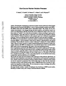
Fig. 1: HCMDP Approach. The lower layer represents the states of the MDP, whereas the higher layer represents the macro-state graph. The blue area shows the set M and is preserved in the two layers.

in the following we present a hierarchical method to accelerate the solution while preserving feasibility and limiting performance loss. IV. HCMDP – H IERARCHICAL C ONSTRAINED M ARKOV D ECISION P ROCESSES Hierarchical methods to solve MDPs have been considered since quite some time (see e.g., [4], vol II, Ch. 6). The principle can be applied to CMDPs too, although to the best of our knowledge this has not been explored yet, with the exception of our recent work [12]. The overarching idea is to create a smaller CMDP (i.e., an instance with fewer states) through clustering of states, compute a policy for the smaller instance, and then utilize this high level strategy to infer a policy for the original problem (see Figure 1). More formally, starting from a CMDP (X, U, P, c, di , Di ), we extract a HCMDP (XH , UH , PH , cH , di,H , Di,H ) with the objective that |X| 0 for 1 ≤ i ≤ n − 1. Let z ∈ X 0 and y ∈ M be two states in the original CMDP, such that z y, and let ZH , yh ∈ XH be the two macro states containing z and y in the hierarchical CMDP. Then, we require that ZH YH . Furthermore, given S ⊂ X, x ∈ X, and a ∈ U (x) we define the following sets a Pre(S) = {x ∈ X|∃a ∈ U (s) ∧ ∃y ∈ S ∧ Pxy > 0} a Post(x, a) = {Y ∈ XH |∃y ∈ Y ∧ Pxy > 0} a Post(S) = {Y ∈ XH |∃y ∈ Y ∧ Pxy > 0}.

Note that Pre(S) is a subset of states of X, whereas Post(x, a) and Post(S) are sets of macrostates of XH . Algorithm 1 illustrates our clustering approach. The algorithm starts by creating a cluster with the absorbing set (line 1). Then, it repeatedly iterates over the set of states that have not been assigned to a cluster, but can reach one of the existing clusters in one step with non-zero probability (line 4). States are then assigned to a cluster if the size of the cluster does not exceed a maximum size (parmeter M S), and the average cost of a cluster is similar to c(s, as ), i.e., the cost incurred in order to move from s into the cluster (lines 6 to 14). We define c(H) as the average of the costs for all the state/action pairs in H. If a state cannot be assigned to any of the existing clusters, then a new cluster with a single state is created (lines 15 to 19), and the process is iterated. At the end, an optional merging step described in the following is performed (line 23). Note that in the current description of the algorithm we assumed that all states are connected to each other and therefore they eventually are all assigned to a cluster. To enforce this property, one can preliminarily identify and eliminate states belonging to components not connected to M . The behavior of the clustering algorithm is defined by two parameters, namely the maximum size of each cluster M S, and the threshold δ used for the test whether c(H) ≈ c(s, as ). The impact of these parameters is evident. Large values for δ lead to clusters of states with dissimilar values for c, thus defying the effectiveness of the clustering approach. On the other hand a too little value leads to too many clusters. In the experimental section we will analyze the sensitivity to M S. The negative effect of a poorly chosen δ is controlled by M S (when δ is too large) or by the merging step (when δ is too small). 1) Merging: Too large clusters negatively impact the performance of the algorithm and the parameter M S is introduced to control this aspect. However, too many small clus-

Algorithm 1: Clustering Algorithm Data: X, U, P Result: XH : Set of macro-states 1 XH ← {M }; 2 while There exist states not assigned to any cluster do 3 foreach C ∈ XH do 4 S ← Pre(C) ∩(X \ ∪XH ) ; 5 foreach s ∈ S do 6 for as ∈ U (s) do 7 Ys ← Post(s, as ); 8 for H ∈ Ys do 9 if c(H) ≈ c(s, as ) ∧ |H| < MS then 10 assign s to cluster H; 11 break out of two nested for loops; 12 end 13 end 14 end 15 if s not assigned yet then 16 create new cluster Ms = {s}; 17 add Ms to XH ; 18 assign s to cluster Ms ; 19 end 20 end 21 end 22 end 23 XH ← merge(XH ); 24 return XH ;

ters also negatively impact the performance. To overcome this problem, small clusters can be combined together during a merging step. A parameter mS (minimum size) is used to trigger the merging process. Algorithm 2 shows how merging is performed. Clusters smaller than mS are combined with neighboring clusters. When multiple neighbors exist, the one with the most similar cost is picked, provided that it does not exceed the maximum size M S. B. Hierarchical Action Set The set of clustered states induces a new set of actions UH for the HCMDP. For a macrostate Y ∈ XH , the action set UH (Y ) is created considering all macrostates that can be reached in one step. Hence, UH (Y ) is: a UH (Y ) = {Z ∈ XH |∃y ∈ Y ∧z ∈ Z ∧a ∈ U (y)∧Pyz > 0}.

Note that UH is induced by XH and the original action set U , but it is made of actions that were not part of U . C. Transition probabilities and costs The final step to complete the construction of HCMDP is the definition of transition probabilities PH , costs cH and di,H , and bounds Di,H . To the best of our knowledge, no principled methods have been proposed to infer these quantities using an analytic approach valid irrespectively

Algorithm 2: Merge Algorithm Data: XH : Set of all macro-states Result: XH : New set of macro-states 1 repeat 2 for M ∈ XH do 3 if |M | < mS then 4 Madj = Post(M) ; 5 Mc ← arg minMc ∈Madj |c(Mc ) − c(M )|; 6 if |Mc | < M S then 7 merge M and Mc and update XH ; 8 end 9 end 10 end 11 until no more states are merged; 12 return XH ;

of the structure of the underlying state space. In order to create a method that can be applied to arbitrary state spaces, we therefore opt for a Monte Carlo based approach in which transition probabilities and costs are estimated through sampling. The advantage of this approach is found in its broad applicability. The known disadvantage is that it does not lend itself to an easy characterization of its performance in terms of analytic bounds. We only describe the estimation method for the transition probabilities, since the idea is similar for the costs. For macro states M1 and M2 and action M3 M3 ∈ U (M1 ) we want to estimate PM . This probability 1 ,M2 is defined only if M1 and M2 are adjacent, i.e., M1 ∈ U (M2 ) and M2 ∈ U (M1 ). The estimation process is as follows. We select one state x ∈ M1 and one state y ∈ M2 . In both cases a uniform random distribution is used. Then we compute the single source shortest path from y using breadth first search. The graph used by BFS has all states in M1 and M2 and has and edge between vertices a ∈ M1 and b ∈ M2 whenever c there is an action c ∈ U (a) such that Pab > 0. Single source shortest path identifies all vertices in M1 reachable from y with a non-zero probability. This set includes x due to the way we built the macro states. By reversing the direction of the edges in the graph we then obtain a policy to go from x to y. Next, a simulation starts, that is we simulate the state evolution from x following the deterministic policy we just computed and using the transition probabilities in the original CMDP. Due to the underlying uncertainty in state evolution, it is possible that while following this policy the state will end in M2 or in a different adjacent macro state. M3 The probability PM is then estimated by taking the ratio 1 ,M2 between the number of times the state eventually reaches M3 and the overall number of attempts. Note that the set M3 of simulations provide also PM with j 6= 2 by counting 1 ,Mj how many times the evolution ends in Mj rather than M2 . Hierarchical costs cH and di,H are estimated using a similar approach. The difference in this case is that the average is taken over the overall costs accrued during the simulation of an application of action Mi from state Mj . Finally, for the hierarchical bounds Di,H we use the same

costs in the original CMDP. This combination of transition probability definition and clustering guarantees connectivity. The proof, omitted for brevity, follows the connectivity proof given in [3]. D. The hierarchical planner Algorithm 3 sketches the structure of the hierarchical planner. The input to the algorithm is the original CMDP, the start state s, and the set of goal states M . The algorithm starts by computing the hierarchical structure (line 1) and then tries solving the associated linear program. If the linear program can not be solved, the various bounds are increased (line 6) and the problem is solved again. We assume all costs are increased, but one could also opt for a different increase strategy, e.g., increasing one at the time. The rationale behind increasing the bounds, is that the hierarchical problem may be unsolvable due to the approximations induced in computing the costs through Monte Carlo sampling (in particular, overestimation of the costs di,H ). Once a strategy for the hierarchical CMDP is found, a sequence of smaller CMDPs is solved to move from one macro state to the next (line 15 to 23). The desired sequence of macro states to follow is given precisely by the policy for the hierarchical problem and exploits our definition of actions for the macro states. In particular, the action set for a macro state YH is given by the set of macro states sharing a boundary with it, so that the goal set computed at line 18 can be easily computed. The cycle terminates when the goal set is reached. Algorithm 3: Algorithmic Sketch Data: CMDP = (X, U, P, c, di , Di ), s, M 1 Build HCMDP (XH , UH , PH , cH , di,H , Di,H ); 2 Solved ← f alse; 3 while Not Solved do 4 Solve LP associated with HCMDP; 5 if LP unfeasible then 6 Increase each bound Di,H of ∆Di,H ; 7 end 8 else 9 Solved ← true; 10 end 11 end ∗ 12 Extract optimal aggregate policy πH (Eq. 3); 13 x ← s; 14 while x ∈ / M do 15 Determine state YH containing s; 16 if YH 6= M then ∗ 17 Z H ← πA (Yt ); 18 GoalSet ← Frontier(YH , ZH ); 19 πL ←SolveLocalCMDP(x, GoalSet); 20 repeat 21 Follow policy πL and update x 22 until x reaches GoalSet or exits YH ; 23 end 24 end

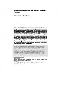
Fig. 2: Sample terrain map. Warmer colors represent high risk areas to be avoided. The right picture shows two different solutions obtained with different risk constraints.

V. E XPERIMENTS AND R ESULTS In this section we experimentally compare three different approaches to solve CMDP problems. The first is the nonhierarchical method that solves the linear program given in Eq. 2. The second is the method we presented in [12] that relies on a fixed structure partitioning of the state space. The third is the method we described in the previous sections, and we study its sensitivity to some of its parameters. As stated in the introduction, our objective is to study high-level motion strategies for autonomous vehicles used in industrial environments while pursuing multiple objectives. High-level in this case means that we abstract from the motion primitives of the vehicle. These can be accounted for in the transition probabilities between states and the associated costs. According to this approach, we focus on planar environments subdivided in regular grids. In this study we assume that cost c is a measure of risk and we consider a single additional cost d representing traveled distance. Our method, however, can include an arbitrary number of additional costs. According to this choice, the problems we study aim at determining paths between couple of points that minimize the overall expected risk while bounding the expected length of the traversed path. We consider two different test cases. The first is shown on the left side of Figure 2. Warmer colors are used to identify cells associated with higher values for the risk cost c. This map is referred to as terrain in the following. The second map is shown in the left side of Figure 3 where black areas are non traversable obstacles and the white area represents free space. Risk is defined as proximity to obstacles which and is shown in the middle panel of the same figure. This map is referred to as maze in the following. In both maps the cost d is set to 1 for every state/action pair. Being defined over a grid, for both environments we assume 4-connectivity and we correspondingly define 4 actions for each state.1 In the state transition model each action succeeds (i.e., the robot moves towards the desired next state) with probability 0.8. For example, if x has four neighbors a and we consider the action a =up, we have Pxy = 0.8 for the state y above x. The remaining 0.2 probability is uniformly spread over x and the three states left, right, bottom. We consider three different performance measures. The first is 1 For states close the boundary or to an obstacle, the action set is adjusted by removing actions that would violate these constraints.

the time spent to find the solution, the second is the value of the objective function c (risk), and the third is the value of the of additional constrained cost d (path length). The code is implemented in Matlab and linear programs are solved using the built in linprog function. To perform a fair time comparison, for the hirarchical methods we log the cumulative time spent inside all the calls to linprog. Table I shows the performance on the terrain environment for 12 different problem instances, where a problem instance is defined as a couple of start and end points (their coordinates are given in figure 4 and 5 on the x axis). The first row of the table shows the timing for the non-hierarchical method (NH) while the second row displays the results for the hierarchical method using fixed partitioning. Successive rows show the results for the algorithm we propose while varying the parameter M S and the sampling rate in the Monte Carlo process. To be specific, X/Y means that the maximum cluster size M S is X, and the number of samples used to estimate probabilities and costs is Y % of the number of states in the clusters. The prefix nm stands for non merged, and indicates that the merging step at the end of Algorithm 1 was not performed. To put the performance of the non-hierarchical method into perspective, we notice that the terrain environment generates a constrained linear program with more than 65000 variables whereas the maze environment induces a linear program with more than 41000 variables. These numbers explain the large difference in time between the non-hierarchical and hierarchical methods, and justify this line of research. Next, we consider the value obtained for the objective function c (risk) and the bounded additional cost d (path length). Results are plotted in Figure 4 and 5 averaging the results of 100 independent runs. The first fact to observe is that the different methods achieve similar performance with regard to the constrained cost d (see Figure 5). This demonstrates that each solution tends to use almost all the allotted budget for d, as specified by the bound D. Considering Figure 4 one observes that, as expected the, non hierarchical method provides the best solution while the other methods in general behave similarly, with a slight better performance for hierarchical solutions using larger clusters. Moreover, instances not using the merging step behave in general worse. Two additional observations are in order. Fixed partitioning appears in general very competitive for this benchmark. However, in some instances it totally fails (like in maze), so it cannot be considered as a generally applicable solution. Second, in some instances (e.g., the second test case in Figure 4) it appears that the non-hierarchical method is outperformed by one of the hierarchical methods. This counterintuitive results is due to the fact that if the linear program for the hierarchical problem is unfeasible, the constraint D is increased (see Algorithm 3). This additional budget for the traversed length may give the possibility to avoid risky areas (high values of c) by taking a detour that is now allowed because of the increased D bound. This aspect is shown in the right panels of Figures 2 and 3. There we show how paths with lower constraints on length are forced

Fig. 3: Maze map where fixed partitioning fails. Left picture shows the map. Middle picture is the risk map associated with the map where the hotter colors illustrate riskier area. The right picture shows two different solutions. Alg NH Fixed 100/10 100/30 100/50 nm/100/50 200/10 200/30 200/50 nm/200/50 400/10 400/30 400/50 nm/400/50

1 107 3.19 4.59 7.04 6.17 5.3 4.9 3.89 4.75 4.03 7.17 6.41 6.80 5.32

2 94.8 2.91 5.49 5.68 8.45 3.48 3.53 3.21 4.50 3.44 6.02 6.83 5.65 3.98

3 54.7 2.2 3.89 4.02 3.79 3.15 4.06 3.74 4.45 3.02 5.25 5.05 5.41 9.72

4 1303.4 1.3 1.72 1.82 1.70 1.76 2.57 2.84 2.38 1.31 5.64 2.52 5.14 6.28

5 613.8 0.8 2.72 1.79 1.65 1.56 1.08 1.49 1.64 1.76 1.71 2.31 2.48 7.16

6 43.9 1.79 2.20 7.33 7.48 2.54 3.47 2.72 2.36 2.63 8.12 8.06 8.09 11.03

6 860.2 2.3 2.43 2.48 2.37 11.84 2.58 2.98 2.48 1.84 3.17 5.43 3.06 4.9

8 86.6 1.5 1.82 3.02 5.48 2.87 3.53 4.01 3.78 4.83 3.76 2.90 2.56 5.92

9 743.9 2.5 3.21 3.59 5.14 2.51 2.9 3.72 5.21 4.07 3.31 4.08 4.39 4.5

10 151.4 0.89 1.43 1.79 2.58 1.92 1.02 1.28 1.21 1.49 2.26 2.42 2.3 2.32

11 59.3 1.89 3.39 3.06 4.34 2.93 3.44 2.84 3.51 2.45 3.45 7.73 3.47 3.83

12 106.2 1.7 2.55 3.59 4.21 2.76 4.57 3.81 3.77 2.20 3.85 4.86 3.89 4.62

TABLE I: Time spent by the various algorithms for the terrain map on 12 different instances.

Fig. 4: Average c cost (risk) over 100 independent runs for the terrain environment. Fig. 5: Average d cost (path length) over 100 independent runs for the terrain environment. through risky areas. We next consider the maze environment. In this case the fixed partitioning method fails because it produces a policy that does not consider the obstacles in the environment (see Figure 6). While this example is specific to the fixed partitioning method we considered, it is easy to show that for any fixed partitioning strategy one can build a state space instance that will be clustered into macro states leading to unfeasible policies. For this reason, adaptive clustering algorithms considering the underlying structure of the state space are needed. These include the one we presented, as well as [3]. Having assessed that our proposed algorithm outperforms the non-hierarchical approach, and that fixed clustering methods are inadequate, the analysis of the maze environment is therefore restricted to the algorithm we proposed. Table II

Fig. 6: Example showing how fixed partitioning fails. Partitions are shown using dotted lines. The hierarchical CMDP induces the policy shown by the red arrows that cannot be executed due to the obstacles cutting through the macro states.

Alg 100/10 100/30 100/50 100/70 100/90 200/10 200/30 200/50 200/70 200/90

1 5.63 3.08 5.69 5.69 5.73 8.52 9.89 9.08 9.62 9.07

2 4.64 3.89 4.54 5.22 4.80 7.95 5.44 8.88 7.51 9.11

3 3.41 3.20 3.76 3.92 3.78 5.05 6.97 5.66 6.37 5.84

4 2.22 2.10 2.54 2.44 2.45 8.48 7.76 6.74 6.28 7.31

TABLE II: Time spent by the various algorithms for the maze map on 4 different instances (in seconds).

of CMDPs. Our method hinges on two steps. A partitioning of the states guaranteed to preserve connectivity, and an estimation of parameters based on Monte Carlo sampling. Our experimental validation confirms that HCMDP offers large gains in terms of computational time while incurring in moderate losses in the objective functions. In the future we aim at deriving bounds for the performance loss. Moreover, by taking advantage of multi-core architectures we will accelerate the estimation of parameters with Monte Carlo sampling by running multiple instances in parallel. R EFERENCES

shows the time spent solving the various instances of linear programs, as we did in Table I. The table confirms that for this metric the size of the cluster is the most relevant parameter, whereas variations are minor when one considers a fixed cluster size and then varies the number of samples. Finally, Figures 7 and 8 show the performance for the functions c and d. The findings confirm what previously observed, i.e., that the performance loss is contained.

Fig. 7: Average c cost (risk) over 100 independent runs for the maze environment.

Fig. 8: Average d cost (path length) over 100 independent runs for the maze environment. VI. CONCLUSIONS In this paper we have presented a hierarchical solution to CMDPs. We believe that the CMDP framework is valuable to the robotics community because it offers a principled solution to multiobjective sequential decision problems and hierarchical solutions are necessary to expedite the solution

[1] E. Altman. Constrained Markov decision processes. CRC Press, 1999. [2] J. Barry, L. P. Kaelbling, and T. Lozano-P´erez. Hierarchical solution of large markov decision processes. Technical report, MIT, 2010. [3] J. L. Barry, L. P. Kaelbling, and T. T. Lozano-P´erez. DetH*: Approximate hierarchical solution of large markov decision processes. In International Joint Conference on Artificial Intelligence (IJCAI), 2011. [4] D. P. Bertsekas. Dynamic programming and optimal control, volume 1,2. Athena Scientific Belmont, MA, 2005. [5] S. Carpin, M. Pavone, and B.M. Sadler. Rapid multirobot deployment with time constraints. In Proceedings of the IEEE/RSJ International Conference on Intelligent Robots and Systems, pages 1147–1154, 2014. [6] Y.-L. Chow, M. Pavone, B.M. Sadler, and S. Carpin. Trading safety versus performance: rapid deployment of robotic swarms with robust performance constraints. ASME Journal of Dynamic Systems, Measurement and Control, 137, 2015. [7] P. Dai and J. Goldsmith. Topological value iteration algorithm for markov decision processes. In Proceedings of the International Joint Conference on Artificial Intelligence, pages 1860–1865, 2007. [8] P. Dai, Mausam, and D. S. Weld. Focused topological value iteration. In International Conference on Automated Planning and Scheduling, 2009. [9] P. Dai, Mausam, D.S. Weld, and J. Goldsmith. Topological value iteration algorithms. Journal of Artificial Intelligence Research, 42(1):181–209, 2011. [10] T. G. Dietterich. Hierarchical reinforcement learning with the maxq value function decomposition. arXiv preprint cs/9905014, 1999. [11] X. C. Ding, A. Pinto, and A. Surana. Strategic planning under uncertainties via constrained markov decision processes. In Proceedings of the IEEE International Conference on Robotics and Automation, pages 4568–4575, 2013. [12] S. Feyzabadi and S. Carpin. Risk aware path planning using hierarchical constrained markov decision processes. In Proceedings of the IEEE International Conference on Automation Science and Engineering, pages 297–303, 2014. [13] J. Hoey, R. St-Aubin, A. J. Hu, and C. C. Boutilier. SPUDD: Stochastic planning using decision diagrams. In Proceedings of Uncertainty in Artificial Intelligence, pages 279–288, 1999. [14] S. M. LaValle. Planning algorithms. Cambridge university press, 2006. [15] T. M. Moldovan and P. Abbeel. Risk aversion in markov decision processes via near optimal Chernoff bounds. In NIPS, pages 3140– 3148, 2012. [16] S. Thrun, W. Burgard, and D. Fox. Probabilistic Robotics. MIT Press, 2006.