since functional programs are significantly easier to check for correctness, why ...... The âeval cardinalâ function performs a loop, expressed as an internal re-.
A Hoare Logic for Call-by-Value Functional Programs Yann R´egis-Gianas1 and Fran¸cois Pottier2 INRIA Saclay - ˆIle-de-France, ProVal, Orsay, F-91893 LRI, Universit´e Paris-Sud, CNRS, Orsay, F-91405 INRIA Paris - Rocquencourt, Gallium - Domaine de Voluceau - F-78153 1
2
Abstract. We present a Hoare logic for a call-by-value programming language equipped with recursive, higher-order functions, algebraic data types, and a polymorphic type system in the style of Hindley and Milner. It is the theoretical basis for a tool that extracts proof obligations out of programs annotated with logical assertions. These proof obligations, expressed in a typed, higher-order logic, are discharged using off-theshelf automated or interactive theorem provers. Although the technical apparatus that we exploit is by now standard, its application to callby-value functional programming languages appears to be new, and (we claim) deserves attention. As a sample application, we check the partial correctness of a balanced binary search tree implementation.
1
Introduction
Hoare logic [1,2,3] is a discipline for annotating programs with logical formulae, known as assertions, and for extracting logical formulae, known as proof obligations, out of such annotated programs. The validity of the proof obligations, which can be verified either manually or mechanically, entails the correctness of the annotated program. That is, it guarantees that the assertions are correct static predictions of the program’s dynamic behavior. Hoare logic was originally designed for a “while language”, that is, a simple imperative programming language, equipped with an iteration construct and a fixed number of global, mutable variables. Recursive, higher-order procedures were the subject of much attention in the late 1970’s and early 1980’s [4,5,6,7,8]. More recently, heap-allocated, mutable data structures, as well as object-oriented features, have been deeply investigated. This has led to the development of practical specification languages and tools targeting, for instance, Java [9,10,11], C [12] and C# [13]. We would like to put forth the thesis that this traditional focus on imperative programming languages has been, to some extent, detrimental: it has consumed a great amount of energy, while comparatively little effort was being devoted to the key features that will be required in order for the methodology to scale up, such as modularity and abstraction. We would also like to raise a question: since functional programs are significantly easier to check for correctness, why hasn’t this activity become routine in the functional programming community, forty years after Floyd and Hoare’s seminal papers?
On the cost of imperative programming There are several reasons why functional programming can be considered superior to imperative programming [14]. One of them is that functional programs are easier to reason about. In other words, there is a cost to reasoning about state. In a typical modern imperative programming language, all heap-allocated data is mutable. As a result, instead of reasoning in terms of high-level entities such as, say, pairs, lists, trees, etc., programmers are forced to reason in terms of a view of the heap as a graph. More concretely, they must write down and prove formulae that involve mappings of memory addresses to memory blocks [15,12]. The possibility of aliasing means that, whenever some memory block is written, the memory that is accessible through every type-compatible pointer is potentially affected. This makes it difficult to reason about the effects of a single write operation, and creates the problem of representation exposure [16,17]. In order to address this issue, researchers have developed linear types and regions [18], ownership types [19], and separation logic [20], among other approaches. Our research agenda We do not claim that the above issues are not worth investigating: on the contrary, they are quite fascinating. However, it is a pity that we do not, today, have mature tools for checking the correctness of functional programs. This explains why, in this paper, we study a Hoare logic for (call-by-value) functional programs without state. The programs that we are interested in checking rely heavily on (possibly higher-order) functions, algebraic data structures, and type polymorphism. We claim that it is quite easy to extract succinct and natural proof obligations out of such programs, provided, of course, that they are annotated with specifications. There are two benefits to be reaped by not reasoning about state. As far as the user is concerned, this leads to simpler specifications and proof obligations. As far as the implementor is concerned, this saves a large part of the “implementation budget”, which can then be spent on features such as type polymorphism, type abstraction, and modularity. The importance of these features cannot be overstated: in the end, the key to success is the ability to develop and check program components independently. Contribution In this paper, we present the design of a typed, polymorphic, higher-order programming language, where programs can be annotated with assertions expressed in a typed, polymorphic, higher-order logic. We define a procedure for extracting proof obligations out of programs, and show that it is sound. A publicly available prototype tool [21] has been developed, which works in conjunction with the interactive theorem prover Coq [22], with the automated first-order theorem prover Alt-Ergo [23], or with both at once. This tool has been used to check the partial correctness of several non-trivial data structure implementations, including balanced binary search trees and purely functional double-ended queues [24]. We hope to publish detailed accounts of these implementations in the future.
Highlights of our approach Here are some of the key technical features of our approach. We focus on partial correctness. We do not require programs to terminate, and do not generate proof obligations to ensure termination. It is up to the user to determine which properties of the code are of sufficient interest to deserve proof, and to insert assertions where desired. At one extreme, a program that contains no assertions leads to no proof obligations. There is no cost to be paid up front for using our methodology. Our preconditions are prescriptive: it is impossible to call a function unless its precondition F1 holds. A descriptive interpretation of preconditions can be simulated by using the precondition true and the postcondition F1 ⇒ F2 . This allows unconditional invocation, and states that the function’s result must satisfy F2 if its argument satisfies F1 . Values, programs, types, and logical formulae are distinct syntactic categories. Proofs do not necessarily appear within programs: proof obligations are delegated to an external theorem prover, which may or may not require or produce explicit proof terms. We do not embed values, programs, or formulae within types. Thus, our types are first-order terms: they include type variables, parameterized algebraic data types, and function types, just as in ML. As a result, type inference in the style of Milner [25] is possible, and implemented in our tool [21]. Type inference does not generate any proof obligations. We do not have dependent types, such as lists indexed with an integer length [26], but simulate them as follows. Instead of declaring that x has type list n, we declare that x has type list, and assert the logical formula length(x) = n, where the function length is inductively defined at the logical level. Formulae can refer to values, but not to expressions. This is important, because values are pure, whereas expressions are potentially impure. Although our logic cannot explicitly reason about state, it is nevertheless soundly applicable to programs that involve non-termination, non-determinism, input/output, or mutable state. (Reading an input stream, or dereferencing a pointer to mutable storage, can be viewed as non-deterministic operations.) In that case, it allows establishing properties that do not depend on the behavior of any impure operation. This means, for instance, that we can prove the partial correctness of a functional program even if it has been instrumented with possibly impure debugging, profiling, or logging instructions. In our programming language, functions, which are potentially impure, are values, so they can appear within formulae. But what does it mean for a formula . to refer to a computational function f of type, say, τ1 −→ τ2 ? Our answer is to view f , at the logical level, as a pair of predicates, which represent f ’s precondition and postcondition. In other words, when used within a formula, f has type (roughly) (τ1 → prop) × (τ1 → τ2 → prop). The two pair projections, written pre and post, can be used to refer to the pair components. That is, pre(f ) and post(f ) offer lightweight notations for referring to f ’s precondition and postcondition. When f is a known (let-bound) function, this mechanism can
be viewed merely as offering abbreviations for known formulae. However, when f is unknown (λ- or ∀-bound), it becomes key to writing natural specifications for higher-order functions (§7.5). In summary, although the technical apparatus that we exploit is by now standard, we believe that it is worth drawing attention to the combination of power and simplicity offered by our technical choices. If extended with a suitable module system, and equipped with a compilation path down to, say, Objective Caml [27], our tool could be used to construct correct purely functional program components, possibly for use within larger, partly imperative programs. Outline of the paper The paper is laid out as follows. First, we briefly introduce a higher-order logic, in which assertions and proof obligations are expressed (§2). Then, we present the syntax and call-by-value semantics of a core functional programming language whose expressions carry explicit assertions (§3). We describe the type system, as well as the procedure for extracting proof obligations out of programs (§4). We present a few extensions of the language (§5) and discuss how proof obligations are transformed for submission to external theorem provers (§6). Last, we present a few excerpts of our balanced binary search tree implementation (§7) and review related work (§8).
2 2.1
The underlying logic Syntax
We rely on a mostly standard higher-order logic [28] whose types and terms appear in Figure 1. Types θ include type variables α, parameterized inductive types, function types, product types, and the type prop of logical propositions. In the following, the syntax of terms is extended with standard syntactic sugar for falsity, disjunction, implication, equivalence, existential quantification, etc. The typing rules appear in Figure 2. In general, we write t for terms of arbitrary type. We write F for formulae, that is, terms of type prop, and P for predicates, that is, terms of type θ → prop. The binary operator #, used in several definitions, expresses the fact that two objects have no common free names. Our logic is not simply-typed. Because our computational language (§3) is polymorphic, and because we wish to lift every computational value up to the logical level, we need polymorphism at the logical level as well. For this reason, we have logical type schemes ς ::= ∀¯ α. θ, where α ¯ is a vector of distinct type ¯ variables. Every occurrence of a variable x is explicitly applied to a type vector θ, which states how the type scheme associated with x is instantiated. For this reason also, we introduce universal quantification over type variables, and use facts of the form ∀¯ α.F . Facts are not formulae: they do not appear in Figure 1. Facts appear only within computational-level type environments Γ (§3.1, Figure 3). The extension of higher-order logic with this very simple form of explicit quantification over types is embedded within the Calculus of Inductive Constructions (§2.2).
θ
ς
∆
::= | | | | ::=
α d θ¯ θ→θ θ×θ prop ∀α. ¯ θ
::= ∅ | ∆, (x : ς) | ∆, α ¯
t, F, P ::= | | | | | | | | | | |
Logical Types Variable Data Function Product Proposition Scheme Logical Type Environments Nil Variable Type Variables
Logical Terms x θ¯ Variable D θ¯ (t, . . . , t) Data λ(x : θ).t Abstraction t(t) Application (t, t) Product π1 Projection (also written pre) π2 Projection (also written post) true Truth t=t Equality t∧t Conjunction ¬t Negation ∀(x : θ).t Universal Quantification
Fig. 1. The logic (syntax)
The logic offers parameterized inductive types. We assume that each inductive type constructor d carries a fixed integer arity, and that every application d θ¯ is arity-consistent. We further assume that d comes with a finite number of data constructors D, each of which is assigned a type scheme of the form: ∀¯ α . θ1 × . . . × θn → d α ¯ We impose a positivity condition [29], which is informally summed up as follows: in the above type scheme, the type constructor d (or any type constructor whose definition is mutually recursive with the definition of d) must not appear under the left-hand side of an arrow within θ1 , . . . , θn . Although there is an introduction form for inductive types, namely the application of a data constructor D, no elimination form is provided here. We can get away with this omission because the process of extracting proof obligations, which is the focus of the present paper, requires no such forms. Of course, when it comes to discharging proof obligations, that is, proving theorems, then inductive definitions and proofs become necessary.
(∆, (x : ς))(x) = ς (∆, (x1 : ς))(x2 ) = ∆(x2 ) if x1 # x2 (∆, α)(x) ¯ = ∆(x) if α ¯ # ∆(x) D : ∀α. ¯ θ1 × . . . × θ n → d α ¯ ¯ i ∀i ∆ ` ti : [ α ¯ 7→ θ]θ ∆ ` D θ¯ (t1 , . . . , tn ) : d θ¯
∆(x) = ∀α. ¯ θ ¯ ∆ ` x θ¯ : [α ¯ 7→ θ]θ ∆ ` t1 : θ1 → θ2 ∆ ` t2 : θ1 ∆ ` t1 (t2 ) : θ2 ∀i
∀i
∆ ` ti : θi
∆ ` t : θ1 × θ2
∆ ` (t1 , t2 ) : θ1 × θ2
∆ ` ti : θ
∆ ` t1 = t2 : prop
∀i
∆, (x : θ1 ) ` t : θ2 ∆ ` λ(x : θ1 ).t : θ1 → θ2
∆ ` πi (t) : θi
∆ ` ti : prop
∆ ` t1 ∧ t2 : prop
∆ ` true : prop ∆ ` t : prop ∆ ` ¬ t : prop
∆, (x : θ) ` t : prop
∆, α ¯ ` t : prop
∆ ` ∀(x : θ).t : prop
∆ ` ∀α.t ¯ : prop
Fig. 2. The logic (type system)
2.2
Interpretation
Our higher-order logic is embedded within the Calculus of Inductive Constructions [29,30], abbreviated to CiC in the sequel. Indeed, each type of our logic can be translated into a term of CiC whose type is Type0 . This guarantees that the translation of polymorphic quantification only introduces type variables of type Type0 in CiC. Each construct of our logic is directly mapped to its counterpart in CiC. This interpretation guarantees that our logic is consistent and validates a number of laws that are used in establishing the soundness of our system (§4.8).
3 3.1
The computational language Syntax
The syntax of our programming language appears in Figure 3. It is equipped with an ML-style type system [25], so types τ and type schemes σ are distinguished. Types include type variables, parameterized algebraic data types, and function . types. We write −→ for the computational function type constructor, so as to distinguish it from the logical function type constructor, written → (Figure 1). We impose a syntactic separation between values and expressions, and require both operands of the function application operator, as well as case scrutinees, to be values. This imposes a style, reminiscent of A-normal form [31], where the result of every intermediate computation is named via a let construct. Of course, such a style is quite user-unfriendly, so, in practice, we offer an unrestricted
τ ::= | | σ ::=
α d τ¯ . τ −→ τ ∀α. ¯ τ
Γ ::= | | |
∅ Γ, (x : σ) Γ, α ¯ Γ, ∀α.F ¯
Computational Types Variable Data Function Scheme Computational Type Environments Nil Variable Type Variables Assumption Values Variable Data Recursive Function
v ::= x τ¯ | D τ¯ (v, . . . , v) | fun f (x : τ /F ) : (x : τ /F ) = e
Patterns Variable Data
p ::= x τ¯ | D τ¯ (p, . . . , p)
e ::= | | |
v v(v) let (x α ¯ : τ /F ) = e in e case v of c
Expressions Value Function Application Local Binding Pattern Matching
c ::= ∅ | (p → 7 e) 8 c
Cases Nil Cons
Fig. 3. The computation language (syntax)
surface language, and automatically translate it down to the kernel language described here. The language supports type inference in the style of Hindley and Milner. However, in this paper, we are not concerned with type inference, so we work with explicitly-typed programs. This is visible (i) in the syntax of values and patterns, where variables and data constructors are annotated with vectors of types that indicate how polymorphic type schemes are instantiated, (ii) at fun and let constructs, where bound variables are annotated with types, and (iii) at let constructs, where a vector of type variables α ¯ can be explicitly bound. A function definition takes the general form: fun f (x1 : τ1 /F1 ) : (x2 : τ2 /F2 ) = e
The symbol / should be read “where”. Every function is recursive, so that f is bound within e. The formal parameter x1 is bound within the precondition F1 , within the postcondition F2 , and within e. The variable x2 , which stands for the result of the function, is bound within the postcondition F2 . We require every function to be annotated with an explicit precondition and postcondition (if missing, true is assumed). A local variable definition takes the general form: let (x α ¯ : τ /F ) = e1 in e2 The local variable x is bound within F and within e2 . The type variables α ¯ are bound within τ , F , and e1 . The proposition F serves as a postcondition for e1 . If it is missing, a default postcondition is assumed, whose definition is deferred to §3.3. A case analysis takes the general form: case v of c Here, c is a possibly empty sequence of cases (i.e., branches). Each branch is of the form (p 7→ e), where the variables that appear in the pattern p are bound within e. Patterns must be linear, that is, a pattern cannot bind a variable twice. 3.2
Lifting computational entities to the logical level
In a Hoare logic, formulae refer to values. That is, if x is bound, at the computational level, by a fun, let, or case construct, then it is possible for a formula F , embedded in the code within the scope of x, to refer to x. This raises two questions: first, if x has computational type τ , what is its logical type, to be used when typechecking F ? Second, if, for the purposes of evaluation, x is substituted with a computational value v, what is the corresponding logical value, to be used when interpreting F ? The problem of lifting types and values to the logical level is trivial in a first-order language. Indeed, the type algebra only contains basic types which are translated to type constants (int is mapped to int). Besides, computational values are essentially first-order terms, interpreted as data in the logic. Yet, in an higher-order language, functions are first-class values. What should be the logical reflection of their code ? We answer these questions by lifting both computational types and computational values up to the logical level (Figure 4). That is, to each computational type τ , we associate a logical type dτ e, and to each computational value v, we associate a logical term dve, with the intended property that if v has computational type τ , then dve has logical type dτ e. Patterns are lifted too. Because patterns form a subset of values, no extra definitions are needed. As announced (§1), computational functions are reflected, at the logical level, as pairs of a precondition and postcondition. This is made explicit in the lifting of computational function types: .
dτ1 −→ τ2 e = (dτ1 e → prop) × (dτ1 e → dτ2 e → prop)
Types dαe = α dd τ¯e = d d¯ τe . dτ1 −→ τ2 e = (dτ1 e → prop) × (dτ1 e → dτ2 e → prop) Type schemes d∀α. ¯ τ e = ∀α. ¯ dτ e Type environments d∅e dΓ, (x : σ)e dΓ, αe ¯ dΓ, ∀α.F ¯ e
= = = =
∅ dΓ e, (x : dσe) dΓ e, α ¯ dΓ e
Values dx τ¯e = x d¯ τe dD τ¯ (v1 , . . . , vn )e = D d¯ τ e (dv1 e, . . . , dvn e) dfun f (x1 : τ1 /F1 ) : (x2 : τ2 /F2 ) = ee = (λ(x1 : dτ1 e).F1 , λ(x1 : dτ1 e).λ(x2 : dτ2 e).F2 )
Fig. 4. Lifting computational types and values to the logical level
The first component of the pair, which represents the function’s precondition, is abstracted over the function’s argument, while the second component, which represents the postcondition, is abstracted over both argument and result. As a result of this definition, if f is bound, at the computational level, to . a function of type τ1 −→ τ2 , then a formula embedded within the code, in the scope of f , views f as a pair of predicates, and can refer to pre(f ) and post(f ). (Recall that, as per Figure 1, pre and post are sugar for the projections π1 and π2 .) Note that f does not denote a logical function. Within a formula, an application f (t) does not make sense: it is ill-typed. Values of computational function type (that is, λ-abstractions) are lifted up to the logical level in a way that is consistent with this definition. A function’s precondition and postcondition alone determine how it is lifted: its code is ignored. (The conformance of a function’s body to its declared pre- and postcondition is checked, of course, via a proof obligation: see rule Fun in Figure 6.) This reflects a philosophy in which the only way of reasoning about the behavior of a function value is via its specification: code never appears within formulae. In order to lift algebraic data types, we lift every algebraic data type definition into an isomorphic inductive type definition. So, for every computationallevel algebraic data type constructor d, there must be a logical-level inductive type constructor, also written d, of identical arity. For every computational-level data constructor D : ∀¯ α. τ1 × . . . × τn → d α ¯,
there must be a logical-level data constructor D : ∀¯ α. dτ1 e × . . . × dτn e → d α ¯. Due to the manner in which computational function types are lifted, the positivity condition (§2) requires the type constructor d to not appear under any side of a computational arrow within τ1 , . . . , τn . This can be a limitation (§9). 3.3
Inferring strongest postconditions
In order to simplify the definition of the procedure that extracts proof obligations, we have required every let construct to carry an explicit postcondition for its left-hand sub-expression (§3.1). In practice, however, annotating every let construct would be quite unpleasant, so it is desirable to construct a reasonable postcondition when the user does not provide one. Ideally, the formula that we should construct in such a situation is the strongest postcondition of the left-hand sub-expression. Our logic is, in fact, sufficiently powerful to express strongest postconditions for every construct in our programming language. For instance, the strongest postcondition for a value v is λx.(x = dve). The strongest postcondition for a function application v1 (v2 ) is post(dv1 e)(dv2 e). We could go on and explain how to construct strongest postconditions for let and case constructs. However, in these two cases, they would be complex formulae, involving existential quantification and disjunction. Eventually, the postconditions carried by let constructs become part of proof obligations, where they appear as hypotheses. For this reason, we do not want them to be too complex: we wish to produce simple, comprehensible proof obligations. Our answer to this issue is to construct strongest postconditions for values and function applications, as suggested above, but not for let and case constructs: instead, we rely on the user-provided postcondition, if there is one, or use the trivial postcondition true, otherwise. In practice, when is it necessary for the user to provide an explicit annotation? The left-hand side of a let construct can be one of four expression forms: a value, a function application, a let form, or a case form. In the first two cases, we do use a strongest postcondition. The third case can be made to never happen, up to a conversion to A-normal form [31]. Only the last case remains. In summary, the only case where our simple-minded approach may call for an explicit, userprovided annotation is that of a let construct whose left-hand sub-expression is a case construct. 3.4
Notions of substitution
Neither types nor formulae influence execution, but do appear in the syntax of values and expressions, in order to allow stating subject reduction and proving the soundness of our Hoare logic. So, the operational semantics reduces expressions that contain explicit types and formulae. To ensure that these annotations
remain consistent as expressions are transformed, we must define a few slightly non-standard notions of substitution. A single type variable α can appear within logical types as well as within computational types. Similarly, a single variable x can appear within formulae as well as within expressions. For this reason, we write [α 7→ τ ] for the substitution that replaces every free occurrence of α at the computational level with τ and every free occurrence of α at the logical level with dτ e. Similarly, we write [x 7→ v] for the substitution that replaces every free occurrence of x at the computational level with v and every free occurrence of x at the logical level with dve. We have annotated let constructs with explicit type abstractions and occurrences of variables with explicit type applications. As a result, contracting a let-redex requires contracting type-level β-redexes as well. In order to do so, we write [x 7→ Λ¯ α.v] for a substitution that replaces every variable occurrence of the form x τ¯ with [¯ α 7→ τ¯]v. Again, this replacement is performed at both computational and logical levels, up to a lifting operation in the latter case. Last, the notation [x 7→ v], which denotes a substitution of a value for a variable, is extended to the notation [p 7→ v], which, when p does not match v, is undefined, and, when p does match v, denotes a simultaneous substitution of values for variables, as follows. The formal definition is: [D τ¯ (p1 , . . . , pn ) 7→ D τ¯ (v1 , . . . , vn )] stands for [p1 7→ v1 ] ∪ . . . ∪ [pn 7→ vn ] Because patterns are linear, this is a union of substitutions whose domains are pairwise disjoint. 3.5
Operational semantics
A standard small-step, call-by-value operational semantics appears in Figure 5. There are three kinds of redexes (β, let, and case) and one evaluation context (the left-hand side of a let construct). An expression is stuck if it is irreducible and not a value. It is easy to check that an expression is stuck if and only if it contains, within an evaluation context, a sub-expression of the form v1 (v2 ), where v1 is not a syntactic function, or of the form case v of ∅.
4
The type system and proof system
We now equip the computational language with an ML-style type system and with a proof system (a Hoare logic), which can be viewed as an algorithm for extracting proof obligations out of well-typed programs. For the sake of succinctness, both are described using a single set of judgements, which assert at once that a program is well-typed and is annotated with consistent formulae. In practice, our tool [21] first checks that the program is well-typed, and, at the same time, infers any omitted type annotations. Then, a set of proof
v1 (v2 ) → [x 7→ v2 ][f 7→ v1 ]e if v1 is fun f (x : τ /F ) : (. . .) = e let (x α ¯ : τ /F ) = v in e → [x 7→ Λα.v]e ¯ case v of (p 7→ e) 8 c → [p 7→ v]e if [p 7→ v] is defined case v of (p 7→ e) 8 c → case v of c if [p 7→ v] is undefined let (x α ¯ : τ /F ) = e1 in e2 → let (x α ¯ : τ /F ) = e01 in e2 if e1 → e01
Fig. 5. Operational semantics obligations, expressed in our typed higher-order logic, is extracted. The fact that the program (including embedded formulae) is well-typed guarantees that the proof obligations are in turn well-typed. 4.1
Environments
The syntax of type environments Γ appears in Figure 3. As is standard, type environments bind variables and type variables. Environments also contain assumptions, that is, formulae that become hypotheses when proof obligations are emitted. An environment of the form Γ, ∀¯ α.F is well-formed when ∀¯ α.F has type prop under dΓ e. 4.2
Proof obligations
A proof obligation is a judgement of the form Γ |= F , where F has type prop under dΓ e. The semantics of the judgment is the validity of the interpretation of F in CiC under the interpretation of the environment Γ , which is decided via an external theorem prover. 4.3
Judgements
The proof system is defined via three judgements, which state properties about values, patterns, and expressions, respectively: Values Γ `v:τ (Figure 6) Patterns Γ `p:τ (Figure 7) Expressions Γ ` e : τ {P } (Figure 8) 4.4
Values
The judgement Γ ` v : τ (Figure 6) states that, under the type environment Γ , the value v has type τ . No precondition or postcondition appear in the judgement. Indeed, because values require no computation, they never have a precondition. Furthermore, because all values can be lifted up to the logical level, they
(Γ, (x : σ))(x) (Γ, (x1 : σ))(x2 ) (Γ, α)(x) ¯ (Γ, ∀α.F ¯ )(x)
Var Γ (x) = ∀α. ¯ τ Γ ` x τ¯ : [α ¯ 7→ τ¯]τ
= = = =
σ Γ (x2 ) if x1 # x2 Γ (x) if α ¯ # Γ (x) Γ (x) Data D : ∀α. ¯ τ1 × . . . × τn → d α ¯ ∀i Γ ` vi : [α ¯ 7→ τ¯]τi Γ ` D τ¯ (v1 , . . . , vn ) : d τ¯
Fun f # F1 , F2 dΓ, (x1 : τ1 )e ` F1 : prop dΓ, (x1 : τ1 ), (x2 : τ2 )e ` F2 : prop . Γ, (f : τ1 −→ τ2 ), f = dfun f . . .e, (x1 : τ1 ), F1 ` e : τ2 {λ(x2 : dτ2 e).F2 } .
Γ ` fun f (x1 : τ1 /F1 ) : (x2 : τ2 /F2 ) = e : τ1 −→ τ2
Fig. 6. The computation language (proof system: values)
don’t need an explicit postcondition: the strongest possible postcondition of a value v is simply equality with dve. Rules Var and Data are straightforward. Rule Fun is more complex. Two premises require the precondition F1 and postcondition F2 to be well-formed formulae, under appropriate environments. The last premise checks that the function’s body conforms to the function’s specification. In order to do so, the type environment is extended with bindings for f and x1 . It is also extended with the hypothesis f = dfun f . . .e, which by definition of lifting (Figure 4) is synonymous for f = (λ(x1 : dτ1 e).F1 , λ(x1 : dτ1 e).λ(x2 : dτ2 e).F2 ). This hypothesis gives meaning to occurrences of pre(f ) and post(f ) within the body of the function, allowing recursive calls to f to be checked. Last, the environment is also extended with the precondition F1 , which means that, within the body of the function, the precondition is assumed to hold. Under this extended environment, the body of the function is required to produce a value that meets the postcondition λ(x2 : dτ2 e).F2 . It is not difficult to see that Γ ` v : τ implies dΓ e ` dve : dτ e. This property is required for the typing rules to construct only well-formed formulae. 4.5
Patterns
The judgement Γ ` p : τ (Figure 7) states that a value of type τ can safely be matched against the pattern p, giving rise to (exactly) the bindings described
Pat-Var (x : τ ) ` x : τ
Pat-Data D : ∀α. ¯ τ 1 × . . . × τn → d α ¯ ∀i Γi ` pi : [α ¯ 7→ τ¯]τi Γ1 , . . . , Γn ` D τ¯ (p1 , . . . , pn ) : d τ¯
Fig. 7. The computation language (proof system: patterns)
Value Γ `v:τ Γ |= P (dve)
App . Γ ` v1 : τ1 −→ τ2 Γ ` v2 : τ1 Γ |= pre(dv1 e)(dv2 e) Γ |= post(dv1 e)(dv2 e) ⇒ P
Γ ` v : τ {P }
Γ ` v1 (v2 ) : τ2 {P }
Let x#P dΓ, α, ¯ (x : τ1 )e ` F : prop Γ, α ¯ ` e1 : τ1 {λ(x : dτ1 e).F } Γ, (x : ∀α. ¯ τ1 ), ∀α.[x ¯ 7→ x α]F ¯ ` e2 : τ2 {P } Γ ` let (x α ¯ : τ1 /F ) = e1 in e2 : τ2 {P }
Case-Nil Γ `v:τ
Γ |= false
Γ ` case v of ∅ : τ 0 {P }
Case-Cons Γ `v:τ Γ0 ` p : τ p # v, P 0 Γ, Γ , dve = dpe ` e : τ 0 {P } Γ, (∀Γ 0 .dve 6= dpe) ` case v of c : τ 0 {P } Γ ` case v of (p 7→ e) 8 c : τ 0 {P }
Fig. 8. The computation language (proof system: expressions)
by Γ . As in ML, these bindings are monomorphic (see Pat-Var). Because patterns are linear, the type environments Γ1 , . . . , Γn in Pat-Data have disjoint domains. 4.6
Expressions
The judgement Γ ` e : τ {P } (Figure 8) states that, under the type environment Γ , the expression e has type τ and (if it terminates) produces a value whose logical reflection satisfies the predicate P . In such a judgement, P has type dτ e → prop under dΓ e. Rule Value directly reflects this intended meaning: the judgement Γ ` v : τ {P } holds if and only if v has type τ under Γ and its logical reflection dve provably satisfies P under the hypotheses found in Γ . The premise Γ |= P (dve) is a proof obligation. Rule App requires the function v1 and its actual argument v2 to have matching computational types. Furthermore, it emits two proof obligations, stating
that (i) the actual argument must satisfy the function’s precondition, and (ii) the function’s postcondition must imply the desired postcondition P . In the last premise, we write P 0 ⇒ P , where P 0 and P have type dτ2 e → prop, for ∀(x : dτ2 e).(P 0 (x) ⇒ P (x)), where x is fresh for P 0 and P . Rule Let checks that e1 has type τ1 and that e1 complies with the postcondition F . Then, the rule performs type generalization, in the style of Milner [25], so that e2 is checked under the assignment (x : ∀¯ α. τ1 ). The hypothesis F is changed into ∀¯ α.[x 7→ x α ¯ ]F , so as to reflect the fact that x now has polymorphic type. In the operational semantics, a let construct behaves just like a β-redex. This suggests that it could perhaps be treated as syntactic sugar, obviating the need for the Let rule. However, this is not possible, for two reasons. One is that let allows type generalization, as explained above, whereas a β-redex does not. The other is that an appropriate postcondition for the function λx.e2 cannot be determined prior to extracting proof obligations: indeed, it has to be λx.P , where P is computed only at extraction time. Rule Case-Nil emits the proof obligation Γ |= false, which requires the conjunction of hypotheses found within Γ to be inconsistent. This ensures that a case construct with zero branches is never executed. Rule Case-Cons requires the value v and the pattern p to have a common type τ . The environment Γ 0 collects the variables bound by p, together with their types. Under the hypothesis that a certain instance of p matches v, which is expressed by extending Γ with Γ 0 and with the hypothesis dve = dpe, the branch e must have the desired type τ 0 and meet the desired postcondition P . Furthermore, under the hypothesis that no instance of p matches v, which is written ∀Γ 0 .dve 6= dpe, the remaining branches must have type τ 0 and meet the postcondition P . (Our use of dpe exploits the fact that patterns form a subset of values, a welcome but unessential property.) When checking a case construct with n branches, the (k + 1)-th branch is checked under the assumption that none of the patterns p1 , . . . , pk match the value v. In particular, for k = n, the conjunction of all hypotheses of the form (∀Γi0 .dve 6= dpi e) is required to be inconsistent. This ensures that control cannot fall off the end of a case construct, or, in other words, that the case analyses are exhaustive. Today’s ML and Haskell compilers implement a sound approximation to this check, using a purely syntactic criterion. We also implement this syntactic criterion: when it succeeds, emitting a proof obligation is unnecessary. 4.7
Algorithmic reading
The judgement Γ ` e : τ {P } defines an algorithm for generating proof obligations. All four parameters of the judgement, namely Γ , e, τ , and P , are inputs of the algorithm, which attempts to build a derivation of the judgement by starting at the root of the expression e and working its way down into the sub-expressions of e. As the algorithm descends, entering fun, let, and case constructs, the environment Γ grows, accumulating new bindings and assumptions. At the same time, the postcondition P is propagated down, in a very straightforward process. At let constructs, this propagation process relies on the (default or user-
provided, see §3.3) annotation in order to determine which postcondition must be propagated into the left-hand sub-expression. The output of the algorithm consists of the proof obligations, of the form Γ |= F , carried by the leaves of the derivation (see Value, App, and Case-Nil). 4.8
Soundness
The soundness of our type system and proof system is established in a standard, syntactic manner. The proofs appear in the first author’s dissertation [32]. It states that the types and logical assertions carried by a program are a sound approximation of its dynamic semantics. Lemma 1 (Environment Weakening). Γ1 , F, Γ2 ` e : τ {P } and Γ1 |= F imply Γ1 , Γ2 ` e : τ {P }. Lemma 2 (Postcondition Weakening). Γ ` e : τ {P1 } and Γ |= P1 ⇒ P2 imply Γ ` e : τ {P2 }. Lemma 3 (Type Substitution). Let φ stand for [¯ α 7→ τ¯]. Then, Γ1 , α ¯ , Γ2 ` e : τ {P } and α ¯ # dom(Γ2 ) imply Γ1 , φ(Γ2 ) ` φ(e) : φ(τ2 ) {φ(P )} Lemma 4 (Value Substitution). Let ρ stand for [x 7→ Λ¯ α.v]. Then, Γ1 , (x : ∀¯ α. τ1 ), Γ2 ` e : τ2 {P } and Γ1 , α ¯ ` v : τ1 and x 6∈ dom(Γ2 ) imply Γ1 , ρ(Γ2 ) ` ρ(e) : τ2 {ρ(P )} Lemma 5 (Pattern Matching). Let ∅ ` v : τ and Γ 0 ` p : τ and p # v. Then, [p 7→ v] is defined if and only if the formula ∃Γ 0 .dve = dpe is valid. Theorem 6 (Subject Reduction). Γ ` e : τ {P } and e → e0 imply Γ ` e0 : τ {P }. Theorem 7 (Progress). ∅ ` e : τ {P } implies that e is either reducible or a value v such that P (dve) is valid.
5
A few extensions
Extra assertions The following construct allows inserting an assertion at an arbitrary point in the code: assert F in e This construct requires F to hold: a proof obligation is emitted. It has no computational content: dynamically, it behaves like e. It is syntactic sugar for let (x : unit/F ) = () in e, where x is fresh. It is particularly useful when our tool is used in conjunction with an automated theorem prover: if the theorem prover fails to discharge a proof obligation, the user can use assert to cut the proof
into smaller, easier steps (if the proof obligation is in fact valid) or to find out what is wrong with the specification (if the proof obligation is in fact invalid). The construct absurd, which statically requires false to hold, marks a piece of code as inaccessible. It is syntactic sugar for a case construct with zero branches. Ghost variables and ghost parameters It is sometimes desirable to explicitly introduce a ghost variable, that is, a name for a witness to an existentially quantified hypothesis. For this purpose, we suggest writing let logic x : θ/F in e This construct binds x within F and e. It requires the assertion ∃(x : θ).F to hold, and introduces F as a new hypothesis into the context. Assertions embedded within e can refer to x, and their proofs can exploit the hypothesis F . However, occurrences of x at the computational level within e are forbidden, since “let logic” has no computational content. Similarly, it is sometimes desirable to abstract a function with respect to a ghost parameter x, like this: fun f [x : θ](x1 : τ1 /F1 ) : (x2 : τ2 /F2 ) = e The brackets bind a ghost parameter x within F1 , F2 , and e. (Again, occurrences of x at the computational level within e are forbidden.) Note that θ can be an arbitrary logical type, so this extension allows explicitly abstracting a function with respect to a proposition or predicate, if desired (see §7.5). Ghost variables and ghost parameters can in principle be viewed as syntactic sugar and translated away [33]. In a realistic implementation, however, they should be primitive notions.
6
Interfacing with external theorem provers
The overall verification process, implemented in our prototype tool, is composed of three main steps. First, type inference translates an implicitly typed source code into an explicitly typed internal language, very similar to the language formalized in §3. Second, the rules of the proof system defined in §4 are applied, producing a set of proof obligations. Third, these proof obligations are turned into goals of the two external provers Coq [22] and Alt-Ergo [23]. We describe this last step in the following. 6.1
Coq
Our typed, higher-order logic is easily embedded within the Calculus of Inductive Constructions, which underlies Coq. As a result, exporting proof obligations to Coq is a simple matter of pretty-printing. Implicit type instantiations
are handled by Coq’s system of implicit arguments. We could have made type instantiations explicit but this would have worsened readability. Coq is an interactive theorem prover. In order to discharge a proof obligation, the user writes a proof script. An open problem is how to maintain these scripts as the source code of the program evolves. The location in the code where a proof obligation arises might change. The statement of a proof obligation might change as well. Perhaps a solution would be to allow only explicitly-stated, explicitlynamed, lemmas to be proved interactively, and to rely solely on an automated theorem prover for discharging anonymous proof obligations, possibly by appeal to an explicit lemma. 6.2
Alt-Ergo
Alt-Ergo [23] is a fully automated theorem prover for a typed, polymorphic, first-order logic. Its design is partly inspired by Simplify [34]. However, AltErgo’s logic is typed and polymorphic, whereas Simplify’s is untyped. This makes Alt-Ergo superior, from our point of view, to Simplify. Indeed, provided our proof obligations lie in the first-order fragment of our logic, they can be directly exported towards Alt-Ergo. If, on the other hand, we wished to use Simplify, we would have to encode our typed, polymorphic logic into Simplify’s untyped logic. Such encodings have been studied [35], but are complex and costly. Of course, the trivial encoding that erases all types is unsound. In addition to first-order logic, Alt-Ergo has native support for linear arithmetic and for the theory of constructors (that is, function symbols f such that f (x) = f (y) implies x = y). The latter is useful for reasoning efficiently about algebraic data structures. In the general case, our proof obligations are most naturally expressed in a higher-order logic, as shown in this paper. However, higher-order logic can be encoded into first-order logic. A standard encoding introduces “apply” predicates that help simulate β-conversion [36]. Perhaps surprisingly, in our case, this encoding can be made to look fairly natural. The symbols pre and post, which so far have stood for the pair projections, can be turned into predicates and simulate not only projection, but also application. Furthermore, we can make pre a binary predicate and post a ternary predicate, avoiding curried function applications. That is, instead of the higher-order formula: f = (λ(x1 : dτ1 e).F1 , λ(x1 : dτ1 e).λ(x2 : dτ2 e).F2 ), we can write: ∀(x1 : dτ1 e).(pre(f, x1 ) ⇔ F1 ) ∧ ∀(x1 : dτ1 e).∀(x2 : dτ2 e).(post(f, x1 , x2 ) ⇔ F2 ) The pair and the three λ-abstractions have been η-expanded, and the projection and application symbols have been fused into applications of pre and post. Provided F1 and F2 are first-order formulae, this is a first-order formula.
type tree = Empty : tree Node : (int × tree × elt × tree) → tree fixpoint elements : tree → set = Empty → empty Node (h, l, x, r) → elements (l) ∪ singleton (x) ∪ elements (r) inductive bst : tree → prop = bst (Empty) ∀ (h, l, x, r). bst (l) and bst (r) and sup (x, elements (l)) and inf (x, elements (r)) ⇒ bst (Node (h, l, x, r))
Fig. 9. Definitions for binary search trees Under this encoding, the definition of the lifting operation on computational types is modified so that the computational function type constructor is no longer interpreted: . . dτ1 −→ τ2 e = dτ1 e −→ dτ2 e .
That is, we make −→ an uninterpreted binary type constructor at the logical level, so that the lifting of types becomes the identity. Thus, in the above formula, . f has logical type τ1 −→ τ2 . The type schemes assigned to pre and post are as follows: .
pre : ∀α1 α2 . (α1 −→ α2 ) × α1 → prop . post : ∀α1 α2 . (α1 −→ α2 ) × α1 × α2 → prop These declarations are admissible by Alt-Ergo. We believe that it should be possible to go a long way with first-order logic alone, even when the program exploits higher-order functions. However, at present, more practical experience is needed in order to support this conjecture.
7
Application: finite sets as binary search trees
As an initial benchmark for our tool [21], we have transcribed Objective Caml’s library implementation of finite sets, represented as balanced binary search trees, into our programming language. The code is presented in the concrete syntax of our prototype implementation. 7.1
Parameters
In the following, we fix a type “elt” of elements. We assume that an algebraic data type “bool”, whose data constructors are “true” and “false”, is available.
let rec mem bst (t, x) where bst (t) returns b where ((b = true) ⇔ (x ∈ elements (t))) = match t with Empty → false Node (h, l, y, r) → if (x = y) then true else if (x < y) then mem bst (l, x) else mem bst (r, x) end
Fig. 10. Membership in a binary search tree
We assume that an equality check over elements, written “=”, is given. It is a . function of computational type elt × elt −→ bool, whose specification could be written as follows: post(=, x1 , x2 , b) ⇔ (b = true ⇔ x1 = x2 ) Similarly, we assume that an ordering relation, written “