STATISTICS, OPTIMIZATION AND INFORMATION COMPUTING Stat., Optim. Inf. Comput., Vol. 3, March 2015, pp 54–65. Published online in International Academic Press (www.IAPress.org)
A Hybrid Bird Mating Optimizer Algorithm with Teaching-Learning-Based Optimization for Global Numerical Optimization Qingyang Zhang, Guolin Yu∗ , Hui Song 1 Research
Institute of Information and System Computation Science, Beifang University of Nationalities, China.
Received: 12 June 2014; Accepted: 10 February 2015 Editor: Yuhong Dai
Abstract Bird Mating Optimizer (BMO) is a novel meta-heuristic optimization algorithm inspired by intelligent mating behavior of birds. However, it is still insufficient in convergence of speed and quality of solution. To overcome these drawbacks, this paper proposes a hybrid algorithm (TLBMO), which is established by combining the advantages of Teachinglearning-based optimization (TLBO) and Bird Mating Optimizer (BMO). The performance of TLBMO is evaluated on 23 benchmark functions, and compared with seven state-of-the-art approaches, namely BMO, TLBO, Artificial Bee Bolony (ABC), Particle Swarm Optimization (PSO), Fast Evolution Programming (FEP), Differential Evolution (DE), Group Search Optimization (GSO). Experimental results indicate that the proposed method performs better than other existing algorithms for global numerical optimization. Keywords Bird Mating Optimizer, Teaching-Learning-Based Optimization, Hybrid Mechanism, Global Numerical Optimization
AMS 2010 subject classifications 90C59,90C26 DOI: 10.19139/soic.v3i1.86
1. Introduction As an open and demanding problem, global numerical optimization is of a great importance in various realword areas. Since a great number of science, engineering and geography problems could be formulated as optimization problems, the efficient and optimization algorithms are always needed to tackle increasingly complex actual problems. Generally speaking, these algorithms can mainly be classified into two categories: traditional techniques and modern heuristic methods. Traditional approaches have been used to solve many practical problems successfully. However, the real-world problems are becoming more and more complex. The large scale optimization issues are associated with multimodality, differentiability and dimensionality. It is too difficult to search the exact optimal value by using traditional algorithms. Thus, modern heuristic techniques with simple and powerful search capabilities aroused the attention of scholars, such as ant colony optimization [1], differential evolution [2], particle swarm optimization [3], simulated annealing [4], artificial bee colony [5] and group search optimizer [6] etc. It has been proved that they are more efficient than traditional techniques in various application fields. Recently, A. Askarzadeh have been proposed a bird mating optimizer (BMO) algorithm based on bird mating phenomenon [7]. Bird mating process is similar to an optimization process in which each bird attempts to breed a quality brood as much as possible. Using distinct patterns to move though the search space is the main difference between BMO and other intelligence algorithms. This feature helps to avoid premature convergence and maintain population diversity. Thus, BMO with simple concept and easy implementation has been successfully applied to ∗ Correspondence to: Guolin Yu (Email: guolin
[email protected]). Research Institute of Information and System Computation Science, Beifang University of Nationalities. China (750021).
ISSN 2310-5070 (online) ISSN 2311-004X (print) c 2015 International Academic Press Copyright ⃝
55
Q. ZHANG, G. YU AND H. SONG
solve different complicated problems. The problem of artificial neural network (ANN) training is solved by BMO, and this method yields better results than the other classifiers [8]. BMO method is proved to be an efficient candidate for estimating the unknown parameters of fuel cell polarization curve [9]. An efficient parameter estimation process is provided by BMO, and the better performance results in gaining the coordinates of the maximum power point (MPP) more accurately [10]. Parameter identification of FC models is solved based on BMO algorithm. Simulation results demonstrate the superior performance of it [11]. BMO algorithm shows promising performance in solving optimization problems. However, it is not efficient in identifying the high performance regions of a solution space. For some complicated problems, BMO shows premature convergence or poor efficiency. Teaching-Learning-Based optimization (TLBO) with fast speed has been widely used to solve kinds of optimization problems successfully [12, 13, 14, 15, 16]. Hence, an effective hybrid algorithm with the advantages of TLBO and BMO, named TLBMO, is proposed to improve solution quality and accelerate the convergence speed. In TLBMO, the two operators of BMO and TLBO are chosen as candidates. Each individual in the current population selects one of them based on probability proportional and generates new potential solutions. In addition, a calculation formula of probability is developed empirically. Five performance criteria are adopted to compare our technique with other existing approaches. The rest of this paper is organized as follows. Bird mating optimizer algorithm is indicated in Section 2. Section 3 shortly summarizes the original TLBO. Our proposed approach is described in detail in Section 4. Numerical simulation results are given in Section 5. Finally, conclusion is presented in Section 6.
2. Bird Mating Optimizer Algorithm BMO is a population-based and evolutionary-based algorithm. The population is called society. Each society member represents a feasible solution, is called bird. Males and females are the main components of the society. The females with the most promising genes, contains parthenogenetic and polyandrous. The males are categorized into three unequal components, namely, monogamous, polygynous and promiscuous. In total, BMO possesses five updating patterns, they are explained below in detail. Monogamy is a mating system that a male bird only mates with a female one. Each monogamous bird selects its interesting female from parthenogenetic and polyandrous by a probabilistic approach and mates with her. The new brood is calculated as follows: → x =x+ω×− r × (xi − x) brood
if
.
r1 > mcf
xbrood (m) = lb(m) − r2 × (lb(m) − ub(m)),
(1)
end
where a 1 × D interesting female individual (xi ) can influence a 1 × D offspring brood (xbrood ) to some extent → depending on the time-varying weight (ω ),D is the dimension of problem,− r denotes a 1 × D vector which each element is a random number with uniform distribution between 0 and 1, mcf is the mutation control factor, distributed between 0 and 1, m is a random number varying 1 and D, ri ’s are random numbers in the range [0, 1], and lb and ub are 1 × D vector which each member denotes the lower and upper bounds of the each dimension of problem, respectively. Polygamy implies a mating system that each polygynous bird chooses several female individuals as partners and mates with them. The offspring brood is calculated from the following equation: xbrood = x + ω × (
K ∑
− → rj . × (xij − x))
j=1
if
(2)
r1 > mcf
xbrood (m) = lb(m) − r2 × (lb(m) − ub(m)), end Stat., Optim. Inf. Comput. Vol. 3, March 2015
56
A HYBRID BIRD MATING OPTIMIZER ALGORITHM
where K is the number of female birds, xij is the j th female bird. Polyandry is also a mating system that several monogamous males are selected for each polyandrous bird probabilistically. The way by which a polygynous bird breeds is same as (2). Promiscuity denotes another mating system in which one male and multiple females have unstable relationships. These birds are generated using a chaotic sequence. The way by which a promiscuous bird breeds is same as (1). Parthenogenesis is the last mating system, means each female can raise brood without the help of males. Each female’s genes are passed to her brood by making a small change in her genes probabilistically. The resultant brood is presented as follows: f or
i=1:D if
r1 > mcf p
xbrood (i) = x(i) + mu × (r2 − r3 ) × x(i),
(3)
end end
where mcf p denotes the mutation control factor,mu is the step size. The steps of BMO are provided as follow: Start
Initialize the population and parameters Calculate the fitness of each individual
Sort individuals
Specify each species
Remove the worst members and generate new ones using chaotic squence Specify elite female for each monogamous individual and produce offspring using Eq. (1) Specify elite female for each polygynous individual and produce offspring using Eq. (2) Specify elite female for each polyandrous individual and produce offspring using Eq. (2) Specify elite female for each promiscuous individual and produce offspring using Eq. (1)
Produce the offspring of each parthenogenetic bird using Eq.(3)
Perform replacement stage
NO
Is the maximum number of fitness evaluations met ?
YES
End
Stat., Optim. Inf. Comput. Vol. 3, March 2015
57
Q. ZHANG, G. YU AND H. SONG
3. Teaching-learning-based optimization TLBO is a new swarm intelligent optimization algorithm, the algorithm mimics teaching-learning phenomenon in classroom. The process of the algorithm mainly includes two parts, Teacher Phase and Learner Phase. Teacher Phase This phase of TLBO mimics the learning of the students through the teacher.During this phase, the teacher spares no effort to move on the average results of the entire classroom up to his or her level in terms of knowledge.xnew and xi denotes 1 × D vectors, D is the dimension of problem, the former are generated by the latter using the following update formula: xnew = xi + r × (xteacher − Tf × xmean ) Tf = round(1 + rand),
(4)
where r is a random number in the range [0, 1], Tf is a teaching factor that can be either 1 or 2. xteacher and xmean are 1 × D vectors which indicates the best individual and the mean of entire population, respectively. Learner Phase This phase means a student increases his or her knowledge with the help of group discussions. Each student (xi )randomly chooses a classmate (xj , j ̸= i)for enhancing his or her knowledge level if the classmate own more knowledge than his or her. { xnew = xi + r × (xj − xi ), if f (xj ) < f (xi ) (5) xnew = xi + r × (xi − xj ), otherwise 4. TLBMO 4.1. Search strategy As mentioned before, the core idea of TLBMO is that two evolution strategies, BMO operators and TLBO mechanisms, are employed to produce new individuals. That is to say, two kinds of strategies can be used for updating current population. We suppose that P c is the probability of employing BMO strategy, the other strategy is employed with the probability of 1 − P c. randi (0, 1) is a random number.If randi (0, 1) is bigger than or equal to P c, BMO operator performs. Otherwise, the TLBO strategy will be employed to generate new individual. In this sense, the abilities of exploration and exploitation are improved effectively. 4.2. Selection probability The ultimate success of an optimization algorithm depends mostly on its ability to keep a good balance between exploitation and exploration. This ability helps algorithm to accelerate the convergence speed and improve the quality of solution. Exploitation means the concentration of the algorithm’s search at the vicinity of current solutions and exploration refers to generates new solutions in as yet untested regions of search space. If a method is unable to keep balance between global and local search, it will be stagnation or get trapped in a local optima. As far as we know that different operator produces different influence on the performance of algorithm. If one operator is emphasized in same phase, some primary information about solution space may be ignored. In the beginning, TLBO operator with powerful exploration ability is employed to expand the solution space. Thus, a larger P c value is employed, because the higher P c values, the higher probability of employing TLBO operator. Thereafter, BMO operator is used to search locally to get the best solution. In order to strengthen the exploitation ability, the P c value is decreasing in the evolution process. In general, each individual has different levels of exploration and exploitation ability in solving various problems. Stat., Optim. Inf. Comput. Vol. 3, March 2015
58
A HYBRID BIRD MATING OPTIMIZER ALGORITHM
Table 1 The pseudo-code of TLBMO method is presented as follows: Algorithm: TLBMO Begin Initialize parameters and halting criterion Generate and evaluate the initial population x While(the halting criterion not satisfied) Sort birds The promiscuous birds are removed and generated by chaotic sequence Calculate the probability P c For each bird xi of the society If randi(0, 1) > P c BMO strategy is used to the current population Else TLBO strategy is applied to the current population End If End For Evaluate and update the offspring End while End Output the obtained global best solution
The selection probability expression is empirically proposed below: (6)
P c(t) = sin(exp(−3t/T )),
where, t and T denotes the current and the maximum number of iteration, respectively. Figure 1 introduces an example of P c assigned for an iteration of 100.
0.9 0.8 0.7 0.6
Pc
0.5 0.4 0.3 0.2 0.1 0
0
20
40 60 the number of iteration
80
100
Figure.1 Probability graph of P c assigned for an iteration of 100. Stat., Optim. Inf. Comput. Vol. 3, March 2015
59
Q. ZHANG, G. YU AND H. SONG
5. Experimental studies 23 benchmark functions are selected to evaluate the performance of TLBMO. A detailed description of these functions is presented in Table 2. These functions are divided into three classes [17]: 1) Unimodal functions f1 − f7 , 2) Basic multimodal functions with several local minima f8 − f13 , and 3) Low-dimensional functions with a few local minima f14 − f23 . 5.1. Experimental setup In all experiments, In order to maintain a comparison as fair as possible, the maximum number of fitness evaluations(M axF ES ) is set to D*10000 for each algorithm [22]. Moreover, all experiments are run 50 times independently. The following parameters are used in this paper: • The control parameters of the ABC algorithm are provided as follows [5]: population size N =20, number of onlookers=number of employed bees=0.5*population size, limit=number of onlookers*D. • The parameter setting of the FEP algorithm is summarized as follows [17]: population size N =100, tournament size q =10, initial η =3. • The parameters of GSO follow the suggestions from [6]: population size N =48, initial head angle φ0 = π4 √ , the constant α = round( D + 1) , maximum pursuit angle θmax = απ2 , maximum turning angle αmax = √n ∑ θmax , the maximum pursuit distance l = ∥U − L∥ = (Ui − Li )2 , where Ui and Li are the upper max 2 i=1
• • • •
and lower bounds for the ith dimension. The parameter of TLBO only requires the population size=50 [15]. For DE, the following parameters are employed [21]: the mutation strategies: “DE/rand/1”, population size N =100, differential amplification factor F = 0.5, crossover probability constant CR = 0.9. According to [19], the parameters of PSO are set as follows: population size N = 40, positive constant c1 = c2 = 1.49445, inertia weight wmax = 0.9, wmin = 0.4. The same parameters are adopted by BMO [7] and TLBMO: population size N = 200, monogamous=100, polygynous=60, promiscuous=20, polyandrous=10, parthenogenetic=10, interesting individual=3, the number of monogamous for polygynous=10, mcf = 0.9, mu= 0.001, wmax = 2.5, wmin = 0.25, mcf pmin = 0.1, mcf pmax = 0.9.
All simulations are implemented on the same platform with Intel Core i5-3210M CPU 2.50GHz, 4G of RAM, and windows7 with MATLAB R2010a. 5.2. Performance criteria This paper employs five performance criteria to evaluate the performance of TLBMO. These criteria are introduced as follows. • Accuracy [22]: The mathematical expression is Accuracy = |F (ˆ x) − F (x∗ )|
(7)
where xˆ is the best solution found by the algorithm in a run,x∗ is the global optimal solution. The minimum accuracy is recorded when reaching the maximum number of function evaluation(M axF ES ). The average and standard deviation of the accuracy values are also calculated. • T estF ES [18]: The criteria records the number of fitness evaluations when the value-to-reach (VTR) is achieved. Stat., Optim. Inf. Comput. Vol. 3, March 2015
60
A HYBRID BIRD MATING OPTIMIZER ALGORITHM
Table 2 the twenty-three benchmark functions used in our study. Test function D ∑
D
S
Minimum
30
[−100, 100]D
0
30
[−10, 10]D
0
xj ) 2
30
[−100, 100]D
0
f4 (x) = max {|xi |}
30
[−100, 100]D
0
30
[−30, 30]D
0
30
[−100, 100]D
0
30
[−1.28, 1.28]D
0
30
[−500, 500]D
-12569.5
30
[−5.12, 5.12]D
0
30
[−32, 32]D
0
30
[−600, 600]D
0
(yi − 1)2 [1 + 10 sin2 (πyi+1 )] + (yi − 1)2 }
30
[−50, 50]D
0
(xi − 1)2 [1 + sin2 (3πxi+1 )]
30
[−50, 50]D
0
2
[−65.536, 65.536]D
1
4
[−5, 5]D
0.0003075
2 2 2
[−5, 5]D [−5, 10] × [0, 15] [−2, 2]D
-1.0316285 0.398 3
3
[0, 1]D
-3.86
6
[0, 1]D
-3.32
4
[0, 10]D
-10
4
[0, 10]D
-10
4
[0, 10]D
-10
f1 (x) = f2 (x) =
f3 (x) =
i=1 D ∑
x2i |xi | +
i=1 D ∑
(
i ∑
D ∏
|xi |
i=1
i=1 j=1
f5 (x) =
1≤i≤D D−1 ∑ i=1 D ∑
(⌊xi + 0.5⌋)2
f6 (x) = f7 (x) = f8 (x) = f9 (x) =
[100(xi+1 − x2i )2 + (xi − 1)2 ]
i=1 D ∑ i=1 D ∑
ix4i + random[0, 1)
√
−xi sin(
|xi |)
i=1 D ∑
[x2i − 10 cos(2πxi ) + 10]
√
i=1
f10 (x) = −20 exp(−0.2 f11 (x) = f12 (x) =
D ∑
1 4000
i=1
x2i −
1 D D ∏
+
D ∑
i=1
1 x2i ) − exp( D
+
i
D−1 ∑
µ(xi , 10, 100, 4)
f13 (x) = 0.1{sin2 (3πx1 ) +
D−1 ∑ i=1
+(xn − 1)[1 + sin2 (2πxn )]} + f14 (x) =
f19 (x) f20 (x) f21 (x) f22 (x) f23 (x)
+
∑25
1
j=1 j+
2 ∑
D ∑
µ(xi , 5, 100, 4)
i=1 ]−1
(xi −aij )6
i=1
x1 (b2 i +bi x2 ) 2 ] b2 +bi x3 +x4 i i=1 1 6 4 2 = 4x1 − 2.1x1 + 3 x1 + x1 x2 − 4x22 + 4x42 5.1 2 5 1 2 = (x2 − 4π 2 x1 + π − 6) + 10(1 − 8π cos xi + 10) 2 = [1 + (x1 + x2 + 1) (19 − 14x1 + 3x21 − 14x2 + 6x1 x2 + 3x22 )]× [30 + (2x1 − 3x2 )2 (18 − 32x1 + 12x21 + 48x2 − 36x1 x2 + 27x22 )] 4 4 ∑ ∑ =− ci exp[− aij (xj − pij )2 ] j=1 i=1 6 6 ∑ ∑ ci exp[− aij (xj − pij )2 ] =− j=1 i=1 5 ∑ [(x − ai )(x − ai )T + ci ]−1 =− i=1 7 ∑ =− [(x − ai )(x − ai )T + ci ]−1 i=1 10 ∑ =− [(x − ai )(x − ai )T + ci ]−1 i=1
f15 (x) = f16 (x) f17 (x) f18 (x)
11 ∑
cos 2πxi ) + 20 + e
i=1
i=1
i=1
1 [ 500
D ∑
xi cos( √ )+1
i=1
π {10 sin2 (πyi ) D
D ∑
[ai −
• Acceleration rate(AR) [18]: This criterion is applied to evaluate a methods convergence speed quantitatively. AR =
T estF EScompetitor , T estF ESM ethod
(8)
Stat., Optim. Inf. Comput. Vol. 3, March 2015
61
Q. ZHANG, G. YU AND H. SONG
where AR < 1 denotes the method is slower than its competitor. • Convergence Graphs [20]: The convergence graphs demonstrate that the mean accuracy performance of total runs, respectively. It is used to measure the convergence speed qualitatively. • Success rate(SR) [20]: The SR is calculated as the number of successful runs to the total number of trials. SR =
# of successf ul runs . total runs
(9)
5.3. Performance of TLBMO In order to present superiority of the new hybrid algorithm, TLBMO is compared with seven existing algorithms. The mean, standard deviation values and t-test for all benchmark functions are counted and listed in Table 3. The values of AR and SR are provided in Table 4. In addition, some representative convergence graphs are presented in Figure 2. The performance of TLBMO is analyzed from the following four aspects. 15
2
10
10 BMO TLBMO PSO GSO ABC DE FEP TLBO
0 10
10
−100 −150
BMO TLBMO PSO GSO ABC DE FEP TLBO
−200 −250 −300 −350
Mean value
0
0.5
1
1.5 FES
2
5
10
−1
10
−2
10 0
10
−3
10 −5
2.5
10
3
−4
0
0.5
1
5
x 10
(a)
1.5 FES
2
2.5
10
3
0
0.5
1
5
x 10
(b)
5
−5
10
0
−10
10
−5
10
0
−5
10
BMO TLBMO PSO GSO ABC DE FEP TLBO
−10
10
−10 −15
10
10
−20
10
−15
0
0.5
1
1.5 FES
(d)
2
2.5
3 5
x 10
10
3 5
x 10
10
10
−15
2.5
10 BMO TLBMO PSO GSO ABC DE FEP TLBO
10 Mean value
0
10
2
5
10 BMO TLBMO PSO GSO ABC DE FEP TLBO
1.5 FES
(c)
5
10
Mean value
0
10
Mean value
Mean value
−50
BMO TLBMO PSO GSO ABC DE FEP TLBO
1
10
Mean value
50
−20
0
0.5
1
1.5 FES
(e)
2
2.5
3 5
x 10
10
0
0.5
1
1.5 FES
2
2.5
3 5
x 10
(f)
Figure.2 Convergence graph of overall algorithms on the selected functions, (a) f1 , (b) f5 , (c) f7 , (d) f9 , (e) f10 , (f) f11 . From Table 3-4 and Figure 2, the following results and analysis can be obtained. • Accuracy analysis: For unimodal functions, from Table 3, it is obvious that TLBMO is able to perform consistently better results than BMO on f1 , f2 , f3 , f4 , f7 , but there are weaker than TLBO. For f5 , there is no significant difference between TLBMO and TLBO, but it is superior to BMO. TLBMO, TLBO and BMO have the same final results on f6 . For multimodal functions with many local minima, from table 3 and figure 2, it is clear that TLBMO is significantly better than BMO and TLBO on function f9 , f12 . For f8 , f13 , TLBMO’s final results are as good as BMO’s and TLBO’s. TLBMO and TLBO can find the global optima on f11 . Stat., Optim. Inf. Comput. Vol. 3, March 2015
62
A HYBRID BIRD MATING OPTIMIZER ALGORITHM
Function f1
f2
f3
f4
f5
f6
f7
f8
f9
f10
f11
f12
f13
f14
f15
f16
f17
f18
f19
f20
f21
f22
f23
a
Index mean std h mean std h mean std h mean std h mean std h mean std h mean std h b/s/w mean std h mean std h mean std h mean std h mean std h mean std h b/s/w mean std h mean std h mean std h mean std h mean std h mean std h mean std h mean std h mean std h mean std h ∑b/s/w b/s/w
TLBMO 1.00e − 052 2.02e − 052 8.25e − 026 8.51e − 026 9.86e − 021 1.82e − 020 6.39e − 019 1.05e − 054 2.13e + 001 1.02e + 000 0 0 7.14e − 004 3.02e − 004
3.51e + 003 7.51e + 002 5.68e − 016 4.02e − 015 3.55e − 015 0 0 0 7.39e − 019 5.21e − 018 2.20e − 003 4.44e − 003 3.84e − 006 7.26e − 012 1.24e − 003 6.59e − 004 4.65e − 008 1.23e − 014 3.58e − 007 3.16e − 012 −6.90e − 014 6.27e − 015 −1.48e − 007 2.24e − 016 8.17e − 002 5.55e − 002 2.04e − 001 1.01e + 000 −4.06e − 005 1.50e − 013 1.34e − 001 9.48e − 001
Table 3 Comparison of TLBMO with different algorithms. BMO PSO GSO ABC 1.11e − 031 5.10e − 186 2.13e − 010 1.2e − 121 7.73e − 031 0 5.82e − 010 3.08e − 121 1 1 1 1 2.00e − 017 1.54e + 002 5.30e − 005 6.41e − 061 9.31e − 017 1.31e + 002 1.50e − 004 8.88e − 061 1 1 1 1 2.28e + 001 1.70e + 003 2.97e + 000 2.61e + 003 1.81e + 001 3.49e + 003 1.90e + 000 5.63e + 002 1 1 1 1 3.96e − 001 1.04e − 007 1.21e − 002 9.81e − 002 3.29e − 001 1.61e − 007 4.15e − 003 3.40e − 002 1 1 1 1 5.24e + 001 1.21e + 005 4.42e + 001 2.14e + 000 4.14e + 001 3.28e + 005 3.68e + 001 3.34e + 000 1 1 1 1 0 2.00e + 002 0 0 0 1.41e + 003 0 0 0 0 0 0 3.26e − 003 2.81e − 003 3.80e − 002 1.65e − 002 1.57e − 003 1.27e − 003 3.04e − 002 3.99e − 003 1 1 1 1 6/1/0 6/0/1 6/1/0 3/1/3 2.19e + 003 2.85e + 003 1.35e − 002 1.34e − 002 3.97e + 002 6.90e + 002 5.34e − 004 7.35e − 012 1 1 1 1 4.82e + 000 5.40e + 001 1.07e + 000 0 2.68e + 000 2.16e + 001 8.96e − 001 0 1 1 1 0 1.78e − 001 3.08e − 001 2.10e − 006 3.42e − 014 4.29e + 000 1.99e + 000 1.92e − 006 4.29e − 015 1 1 1 1 1.53e − 003 1.59e − 002 1.83e − 002 1.48e − 003 3.91e − 003 2.22e − 002 1.65e − 002 4.51e − 003 1 1 1 1 3.82e − 014 4.15e − 003 1.26e − 013 1.57e − 032 2.70e − 013 2.05e − 002 2.02e − 013 5.53e − 048 1 1 1 1 1.76e − 003 1.32e − 003 8.51e − 012 1.35e − 032 4.06e − 003 3.61e − 003 4.13e − 011 1.11e − 047 1 1 1 1 4/0/2 4/0/2 5/0/1 2/0/4 3.84e − 006 3.84e − 006 3.84e − 006 3.84e − 006 0 1.19e − 016 2.08e − 016 8.62e − 017 1 1 1 1 1.56e − 003 1.63e − 003 1.50e − 003 1.13e − 003 6.07e − 004 2.26e − 003 2.26e − 003 3.48e − 004 0 0 0 0 4.65e − 008 4.65e − 008 4.65e − 008 4.65e − 008 0 5.33e − 017 6.73e − 017 8.22e − 017 1 1 1 1 3.58e − 007 3.58e − 007 3.58e − 007 3.58e − 007 0 0 7.41e − 013 0 1 1 1 1 −7.78e − 014 −7.75e − 014 −7.37e − 014 6.40e − 006 7.86e − 016 1.23e − 015 3.56e − 015 3.94e − 005 1 1 1 0 −1.48e − 007 −1.48e − 007 −1.48e − 007 −1.42e − 007 0 8.79e − 017 2.89e − 016 2.76e − 008 1 1 1 0 9.78e − 002 4.23e − 002 4.29e − 002 1.99e − 006 4.63e − 002 6.40e − 002 5.78e − 002 1.72e − 016 0 1 0 1 1.21e + 000 4.69e + 000 2.02e + 000 1.10e − 005 2.32e + 000 2.09e + 000 2.92e + 000 4.59e − 005 1 1 1 1 3.60e − 001 3.20e + 000 2.94e + 000 3.63e − 004 1.48e + 000 3.09e + 000 3.41e + 000 1.74e − 003 1 0 1 1 1.53e − 001 2.43e + 000 2.38e + 000 5.98e − 005 1.08e + 000 3.22e + 000 3.26e + 000 3.55e − 004 1 1 1 1 5/4/1 4/4/2 4/4/2 3/3/4 15/5/3 14/4/5 15/5/3 8/4/11
TLBO 0 0 1 4.12e − 278 0 1 3.80e − 091 2.66e − 090 1 2.32e − 222 0 1 1.02e + 001 1.95e + 000 1 0 0 0 2.02e − 004 6.92e − 005 1 0/1/6 2.93e + 003 6.48e + 002 1 6.45e + 000 5.50e + 000 1 3.55e − 015 0 0 0 0 0 2.07e − 003 1.47e − 002 1 2.96e − 002 4.22e − 002 1 3/2/1 3.84e − 006 1.03e − 013 1 9.67e − 004 6.55e − 004 1 4.65e − 008 1.36e − 016 1 3.58e − 007 9.16e − 015 1 −7.77e − 014 6.96e − 016 1 −1.48e − 007 0 1 1.08e − 002 3.27e − 002 1 9.39e − 002 6.55e − 001 0 1.72e − 001 8.11e − 001 1 1.10e − 001 7.77e − 001 1 2/4/4 5/7/11
DE 2.29e − 036 3.31e − 036 1 5.98e − 014 3.27e − 013 1 1.52e − 005 1.42e − 005 1 3.03e − 001 6.25e − 001 1 4.85e − 002 7.11e − 002 1 0 0 0 4.47e − 003 1.16e − 003 1 5/1/1 3.98e + 003 9.51e + 002 1 1.38e + 002 2.52e − 001 1 3.91e − 015 1.08e − 015 1 3.45e − 004 2.44e − 003 0 1.57e − 032 5.53e − 048 1 1.35e − 032 1.11e − 047 1 5/0/1 3.84e − 006 1 1 1.13e − 003 6.25e − 004 1 4.65e − 008 4.40e − 017 1 3.58e − 007 0 1 −7.89e − 014 9.26e − 016 1 −1.48e − 007 0 1 1.03e − 001 4.18e − 002 0 3.21e − 007 0 1 −4.06e − 005 8.61e − 016 1 −9.82e − 006 2.51e − 016 1 0/5/5 10/6/7
FEP 5.30e − 008 3.75e − 007 1 1.24e − 004 8.74e − 004 1 8.40e − 001 5.94e + 000 1 3.36e − 002 2.38e − 001 1 9.21e − 001 6.51e + 000 1 0 0 0 2.80e − 004 1.98e − 003 1 4/1/2 1.24e + 004 1.57e + 003 1 5.97e − 002 4.22e − 001 0 2.27e − 005 1.61e − 004 1 1.56e − 003 1.10e − 002 0 4.65e − 010 3.29e − 009 1 6.78e − 009 4.79e − 008 1 5/0/1 7.68e − 008 5.43e − 007 1 3.78e − 005 2.67e − 004 1 4.83e − 005 3.41e − 004 1 8.46e − 005 5.99e − 004 1 8.96e − 012 6.34e − 011 1 1.09e − 002 7.73e − 002 0 1.69e − 002 1.20e − 001 1 1.02e − 001 7.21e − 001 1 1.06e − 001 7.52e − 001 1 1.08e − 001 7.65e − 001 1 5/0/5 14/1/8
b/s/w indicates that TLBMO wins in b functions, tie in s functions and loses in w functions, compared with its competitors.
Stat., Optim. Inf. Comput. Vol. 3, March 2015
63
Q. ZHANG, G. YU AND H. SONG
For multimodal functions with a few local minima, as indicated in table 3, there are no obvious difference between TLBMO and its competitors. • Signif icance analysis: In order to explain the statistical significance of TLBMO, the Wilcoxon signedrank test is employed. The numerical values “1” means that TLBMO is statistically inferior to other algorithms,“0” represents that TLBMO is equal to its competitor. The total number of TLBMO performs better, similar or worse than other algorithms are summarized in the last row of Table 3. The results demonstrate that there is significantly difference between TLBMO and BMO on the majority of test functions. The mean values of the final solutions reconfirm that the difference between them is not obvious.
Function
Index
f1
AR SR AR SR AR SR AR SR AR SR AR SR AR SR AR SR AR SR AR SR AR SR AR SR AR SR AR SR AR SR AR SR AR SR AR SR AR SR AR SR AR SR AR SR AR ∑SR SR
f2 f3 f4 f5 f6 f7 f8 f9 f10 f11 f12 f13 f14 f15 f16 f17 f18 f19 f20 f21 f22 f23
Table 4 Comparison of TLBMO and its competitor. TLBMO BMO PSO GSO ABC TLBO 1 1 1 1 0 1 0.86 1 1 1 1 1 0.72 1 0.40 1 1 1 1 0.30 0.96 1 0.98 20.20
1.29 1 1.03 1 0 0 0 0 N aN 0 2.16 1 0 0 1 1 0.03 0.02 0.03 0.02 1.05 0.84 1.00 1 1.05 0.84 0.97 1 0.48 0.24 0.96 1 0.82 1 0.73 1 0.92 1 0.25 0.18 0.62 0.76 0.74 0.94 0.81 0.98 14.80
1.02 1 0.19 0.22 0.90 0.76 0.44 0.24 N aN 0 1.51 0.98 0.03 0.02 0.21 1 0 0 0.82 0.96 0.33 0.34 0.74 0.96 0.81 0.88 0.83 1 0.40 0.38 0.89 1 0.75 1 0.95 1 0.82 1 0.58 0.68 0.11 0.14 0.41 0.46 0.61 0.62 13.70
1.59 1 0 0 0 0 0 0 N aN 0 0.80 1 0 0 0.25 1 0.20 0.14 0 0 0.32 0.02 0.63 1 1.05 1 0.50 1 0.64 0.62 0.21 1 0.32 1 0.28 1 0.40 1 0.22 0.64 0.40 0.66 0.23 0.56 0.61 0.64 13.50
0.39 1 0.44 1 0 0 0 0 N aN 0 0.37 1 0 0 0.11 1 0.35 1 0.47 1 0.46 0.88 0.28 1 0.35 1 0.48 1 0.88 0.44 0.35 1 0.45 1 1.25 0.92 0.72 1 0.43 1 0.46 1 0.58 0.94 0.71 0.96 18.10
0.08 1 0.10 1 0.23 1 0.09 1 N aN 0 0.06 1 0.28 1 0.26 1 0.14 0.24 0.09 1 0.09 1 0.37 0.98 0.17 0.28 1.42 1 0.56 0.56 0.63 1 0.70 1 0.60 1 0.70 1 1.11 0.84 1.09 0.96 1.13 0.94 1.07 0.98 19.80
DE
FEP
1.14 1 1.56 1 0 0 0 0 N aN 0 0.87 1 0 0.02 0.51 1 0 0 1.25 1 1.09 0.98 0.82 1 1.01 1 1.27 1 0.24 0.24 0.86 1 0.97 1 0.58 1 0.82 1 0.18 0.14 0.51 1 0.63 1 0.68 1 16.40
0 0.98 0 0.98 0 0.98 0 0.98 N aN 0.98 0.06 1 0 0.98 0.01 1 0 0.98 0 0.98 0 0.98 0 0.98 0 0.98 0.04 1 0 0.98 0 0.98 0 0.98 0.05 1 0 0.98 0 0.98 0 0.98 0 0.98 0 0.98 22.60
• Convergence speed: Table 4 show that TLBMO converges faster than BMO, especially for function f6 . For example, compared with BMO, the AR value is 1.05, which means that TLBMO is on average 5% faster Stat., Optim. Inf. Comput. Vol. 3, March 2015
64
A HYBRID BIRD MATING OPTIMIZER ALGORITHM
than BMO for f11 function. Additionally, Figure 2 shows that TLBMO is able to converge to better solutions quickly and it has higher accuracy than BMO on the most of functions. From figure 2. it is clear that TLBO is significantly superior to all the other methods including TLBMO in the process of evolution, while TLBMO performs the second best on this benchmark function. Looking carefully at Figure 2 (c), PSO shows a faster convergence rate initially than TLBMO, however, it is outperformed by TLBMO after 25000 FES. we can observe from Figure 2 (d) that all the other algorithms show the almost same startpoint, and ABC has a faster convergence speed than other methods. Although slower, TLBMO eventually finds the global solution close to ABC. Totally, the convergence speed of BMO is improved in a certain extent. • Success ratio: Table 4 reveals that the TLBMO has more superior searching ability than its competitors, and ∑ provides the much higher successful rate SR = 20.20 than other existing algorithms. To be specific, our algorithm can effectively solve (SR = 1) seventeen out of twenty-three test functions. It is worth mentioning that TLBMO can yield the smallest mean value with SR = 1 on function f11 and f22 . In general, the hybrid method is able to form stable search mechanism.
6. Conclusion In order to accelerate the convergence speed and improve solution quality of BMO, a hybrid algorithm, named TLBMO, is proposed. This method can provide a better balance between exploration and exploitation in the evolving process. The performance of TLBMO algorithm is verified on a comprehensive set of well-known 23 benchmark functions. Experimental results demonstrate the good performance of TLBMO.
Acknowledgement The authors would like to thanks Prof. Alireza Askarzadeh for providing the BMO code and also to extend sincere gratitude to Prof. Yuhong Dai for his free-handed assistance. This work was supported by Natural Science Foundation of China under Grant No. 11361001; Ministry of Education Science and technology key projects under Grant No. 212204; Natural Science Foundation of Ningxia under Grant No. NZ12207; The Science and Technology key project of Ningxia institutions of higher learning under Grant No. NGY2012092.
REFERENCES 1. M. Dorigo, and T. Stutzle, Ant colony optimization., MAMIT Press. Cambridge, 2004. 2. R. Storn, and K. Price, Differential evolution-a simple and efficient heuristic for global optimization over continuous spaces, Joural of Global optimization, vol. 11, pp. 341-359, 1997. 3. J. Kennedy, and R. Eberhart, Particle swarm optimization, IEEE International conference on Neural Networks, pp. 1942-1948, 1995. 4. S. Kirkpatrick, C. D. Gelatt and M. P. Vecchi, Optimization by simulated annealing, Science, vol. 220, pp. 671-680, 1983. 5. D. Karaboga, An idea based on honey bee swarm for numerical optimization, Technical report-tr06, Kayseri, Turkey: Erciyes University, 2005. 6. S. He, Q. H. Wu and J. R. Saunders, Group search optimizer: an optimization algorithm inspired by animal searching behavior, IEEE Transactions on Evolutionary Computation, vol. 13, pp. 973-990, 2009. 7. A. Askarzadeh, An optimization algorithm inspired by bird mating strategies, Communication in Nonlinear Science and Numerical Simulation, vol. 19, pp. 1213-1228, 2014. 8. A. Askarzadeh, and A. Rezazadeh, Artificial neural network training using a new efficient optimization algorithm, Applied Soft Computing, vol. 13, pp. 1206-1213, 2013. 9. A. Askarzadeh, Parameter estimation of fuel cell polarization curve using BMO algorithm, International Journal of Hydrogen Energy, vol. 38, pp. 15405-15413, 2013. 10. A. Askarzadeh, and A. Rezazadeh, Extraction of maximum power point in solar cells using bird mating optimizer-based parameters identification approach, Solar Energy, vol. 90, pp. 123-133, 2013. 11. A. Askarzadeh, and A. Rezazadeh, A new heuristic optimization algorithm for modeling of proton exchange membrane fuel cell: bird mating optimizer, International Journal of Energy Research, vol.37, pp. 1196-1204, 2013. 12. R. V. Rao, and V. Patel, Multi-objective optimization of two stage thermoelectric cooler using a modified teaching-learning-based optimization algorithm, Engineering Applications of Artificial Intelligence, vol. 26, pp. 430-445, 2013. Stat., Optim. Inf. Comput. Vol. 3, March 2015
Q. ZHANG, G. YU AND H. SONG
65
13. R. V. Rao, and V. Patel, An improved teaching-learning-based optimization algorithm for solving unconstrained optimization problems, Scientia Iranica, vol. 20, pp. 710-720, 2013. 14. R. V. Rao, and V. Patel, D. P. Vakharia. Teaching-Learning-Based Optimization: An optimization method for continuous non-linear large scale problems, Information Sciences, vol. 183, pp. 1-15, 2012. 15. R. V. Rao, and V. Patel, D. P. Vakharia. Teaching-learning-based optimization: An novel method for constrained mechanical design optimization problems, Computer-Aided Design, vol. 43, pp. 303-315, 2011. 16. R. V. Rao, and V. D. Kalyankar, Parameter optimization of modern machining process using teaching-learning-based optimization algorithm, Engineering Applications of Artificial Intelligence, vol. 26, pp. 524-531, 2013. 17. X. Yao, Y. Liu, and G. M. Linm, Evolutionary Programming Made Faster, IEEE Transactions on Evolutionary Computation, vol. 3, pp. 82-102, 1999. 18. W. Y. Gong, Z. H. Cai, and C. X. Ling, DE/BBO: A hybrid differential evolution with biogeography-based optimization for global numerical optimization, Available from: http://embeddedlab.csuohio.edu/BBO/. 19. J. J. Liang, A. K. Qin, P. N. Suganthan, and S. Baskar, Comprehensive learning particle swarm optimizer for global optimization of multimodal functions, IEEE Transactions on Evolutionary Computation, vol. 10, no. 3, pp. 281-295, 2006. 20. W. Y. Gong, Z. H. Cai, C. X. Ling, and H. Li, Enhanced differential evolution with adaptive strategies for numerical optimization, IEEE Transactions on Evolutionary Computation, vol. 41, pp. 397-413, 2011. 21. S. Rahnamayan, H. R.Tizhoosh, and M. A. Salama, Opposition-based differential evolution, IEEE Transactions on Evolutionary Computation, vol. 12, pp. 64-79, 2008. 22. P. N. Suganthan, N. Hansen, and J. J. Liang, et al, Problem definitions and evaluation criteria for CEC 2005 special session on real-parameter optimization, http://www.ntu.edu.sg/home/epnsugan.
Stat., Optim. Inf. Comput. Vol. 3, March 2015