Maryam Daneshmandi et.al / Indian Journal of Computer Science and Engineering (IJCSE)
A Hybrid Data Mining Model to Improve Customer Response Modeling in Direct Marketing Maryam Daneshmandi
[email protected] School of Information Technology Shiraz Electronics University Shiraz, Iran
Marzieh Ahmadzadeh
[email protected] School of Computer Engineering & IT Shiraz University of Technology Shiraz, Iran Abstract Direct marketing is concerned with which customers are more likely to respond to a product offering or promotion. A response model predicts if a customer is going to respond to a product offering or not. Typically historical purchase data is used to model customer response. In response modeling customers are partitioned in to two groups of respondents and non-respondents. Generally, the distribution of records (respondents and nonrespondents) in marketing datasets is not balanced. The most common approach to solve class imbalance problem is by using sampling techniques. However; sampling techniques have their shortcomings. Therefore, in this research we integrated supervised and unsupervised learning techniques and presented a novel approach to address class imbalance problem. Recently hybrid data mining techniques have been proposed and they intend to improve the performance of the basic classifiers. Finally we compared the performance of the hybrid approach to that of the sampling approach. We could show that the hybrid ANN model achieved higher prediction accuracy and higher area under the curve value than the corresponding values of the bagging neural network which was trained based on the sampled training set. Keywords: Response Modeling, Direct Marketing, Supervised learning, Unsupervised Learning, Hybrid Models, Neural Networks 1. Introduction and Related Work In general, businesses worldwide use mass marketing as their marketing strategy for offering and promoting a new product or service to their customers. The idea of mass marketing is to broadcast a single communication message to all customers so that maximum exposure is ensured. However; since this approach neglects the difference among customers it has several drawbacks. In fact a single product offering cannot fully satisfy different needs of all customers in a market and unsatisfied customers with unsatisfied needs expose businesses to challenges by competitors who are able to identify and fulfill the diverse needs of their customers more accurately. Thus in today’s world where mass marketing has become less effective, businesses choose other approaches such as direct marketing as their main marketing strategy(HosseinJavaheri 2007). Direct marketing is concerned with identifying which customers are more likely to respond to specific promotional offers. A response model predicts the probability that a customer is responsive/non-responsive to an offer for a product or service. A response modeling is usually the first type of target modeling that a business develops as its marketing strategy. If no marketing promotion has been done in the past, a response model can make the marketing campaign more efficient and might bring in more profit to the company by reducing mail expenses and absorbing more customers(Parr Rud 2001). Response model can be formulated in to a binary classification problem in which customers are divided in to two groups of respondents and non-respondents. Typically historical purchase data is used to model customer response. In direct marketing a desirable response model should contain more respondents and fewer non-respondents(Shin 2006). Various data mining techniques have been used to model customer response to catalogue advertising. Traditionally statistical methods such as discriminant analysis, least squares and logistic regression have been applied to response modeling. However, since statistical measures such as logistic regressions are limited in that the models are linear in parameters, other approaches have been proposed. Haughton and Oualbi modeled the response lift of CART and CHAID, which are decision tree algorithms. They found that CART and CHAID perform in a remarkably similar way as far as lift in response is concerned(Haughton and Oualabi 1997).
ISSN : 0976-5166
Vol. 3 No.6 Dec 2012-Jan 2013
844
Maryam Daneshmandi et.al / Indian Journal of Computer Science and Engineering (IJCSE)
Neural Networks have also been used in response modeling. Bounds and Ross showed that neural networks could improve the response rate from 2% up to 95%(Bounds 1997). Viaene et al have also used neural networks to select input variables in response modeling(Viaene, Baesens et al. 2001). Ha et al applied bagging neural networks to propose a response model. They used dataset DMEF4 and compared this approach to Single Multilayer Perception (SMLP) and Logistic Regression (LR) in terms of fit and Performance. They could show that bagging neural network outperformed the SMLP and LR(Ha, Cho et al. 2005). Tang applied feed forward neural network to maximize performance at desired mailing depth in direct marketing in cellular phone industry. He showed that neural networks show more balance outcome than statistical models such as logistic regression and least squares regression, in terms of potential revenue and churn likelihood of a customer(Tang 2011). Bentz and Merunkay also showed that neural networks did better than multinomial logistic regression(Bentz 2000). To overcome the neural networks limitations, Shin and Cho applied Support Vector Machine (SVM) to response modeling. In their study, they introduced practical difficulties such as large training data and class imbalance problem. When applying SVM to response modeling. They proposed a neighborhood property based pattern selection algorithm (NPPS) that reduces the training set without accuracy loss. NPPS selects the patterns in the region around the decision boundary based on the neighborhood properties. For the other remaining problem they employed different misclassification costs to different class errors in the objective function(Shin 2006). Recently, Hybrid data mining approaches have gained much popularity; however, a few studies have been proposed to examine the performance of hybrid data mining techniques for response modeling. A hybrid approach is built by combining two or more data mining techniques. A hybrid approach is commonly used to maximize the accuracy of a classifier. Coenen et al proposed a hybrid approach with C5, a decision tree algorithm and case based reasoning (CBR). In their study, First cases were classified by means of C5 algorithm and then the classified cases were ranked by a CBR similarity measure. This way they succeeded to improve the rank of the classified cases(Coenen 2000). Chiu also proposed a CBR system based on Genetic Algorithm to classify potential customers in insurance direct marketing. The proposed GA approach determines the fittest weighting values to improve the case identification accuracy. The created model showed better learning and testing performance(Chiu 2002). Building an effective response model has become an important topic for businesses and academics in recent years. The purpose of this study is to develop a hybrid data mining model by integrating supervised and unsupervised data mining techniques. A hybrid model can improve the performance of basic classifier(Tsai 2009). The following sections are organized as follows. Section 2 briefly explains the benefit of hybrid techniques and the data mining techniques which are used in this article. In section 3 we introduce two approaches we propose in this paper to solve class imbalance problem, ,the dataset used in this research, experimental settings and performance measurements respectively. Finally we concluded the paper in section 4 with some recommendations for future work. 2. Supervised vs. Unsupervised Learning Machine learning algorithms are described as either ‘supervised’ or’ unsupervised’. The distinction is drawn from how the classifier classifies data. The unsupervised learning sometimes referred to as clustering, the unsupervised classification of records into different groups or clusters based on similarity. Records within the same cluster are expected to be similar to one another, whereas the records between clusters are assumed to be different. In supervised learning, sometimes referred to as classification, the classes are predetermined therefore a collection of labeled instances are available. The problem is to label newly encountered instances whereas in unsupervised learning the challenge is to group a collection of unlabeled instances in to clusters and find hidden structures in unlabeled data(Berry and Brown 2006). 2.1. Hybrid approaches (Combination of Supervised and Unsupervised Learning) In general, hybrid models are built by combining two or more data mining techniques in order to use the strength of different classifiers and increase the performance of the basic classifiers. For instance, supervised and unsupervised techniques can be serially integrated.” That is, clustering can be used as a pre-processing stage to identify pattern classes for subsequent task of supervised prediction or classification(Jain 1999)”. Hence, clustering can be used to identify homogenous populations in the data set. Then each cluster becomes a training set to train and finally a classification model can be created for the desired clusters. (Tsai 2009). The combination of supervised and unsupervised learning algorithms is a recent approach in the field of machine learning. Such a combination can either be used to improve the performance of a supervised classifier by biasing the classifier to use the information coming from the supervised classifier or it can be used to incorporate large amount of unlabeled data in the supervised learning process. Both methods can be performed
ISSN : 0976-5166
Vol. 3 No.6 Dec 2012-Jan 2013
845
Maryam Daneshmandi et.al / Indian Journal of Computer Science and Engineering (IJCSE)
either simultaneously, which is referred to as internal, or independently, which is referred to as external (Japkowicz). In this research we combined supervised and unsupervised learning to bias the information fed to the supervised classifier. Since the unsupervised learning was first done followed by the supervised learning, it can be referred to as an external method. The data mining algorithms applied in this research are briefly stated below: 2.1.1 K-Means Clustering Algorithm K-Means is one of the simplest unsupervised learning algorithms that solves the well-known problem of clustering. K-Means requires the number of clusters as an input. K-Means steps for clustering are listed below: 1. Decide on a value for k 2. Initialize the K cluster centers 3. Form K clusters by assigning each point to the nearest cluster. 4. Recompute the center of each cluster Repeat step 3 and step 4 until the centers no longer change(Tan. P., Steinbach. M. et al. 2006). 2.1.2 Two Step Clustering Algorithm The algorithm can handle very large datasets. It is also designed to handle both continuous and categorical variables. It uses an agglomerative hierarchical clustering and involves two steps: including Preclustering and Clustering. Preclustering step: The first step makes a single pass through the data. Two Step applies a log-likelihood distance measure to calculate distance between cases. In preclustering step records are scanned one by one and based on the distance measure decides if the current record should be merged with the previously formed cluster or starts a new cluster. Clustering step: The second step uses a hierarchical clustering method to progressively merge the sub clusters into larger clusters, without requiring another pass through the data(Spss Algorithms Guide 2009). 2.1.3. C&R Tree Classification Algorithm Classification and regression trees (C&R Tree) divide the data in to two subsets in a way that the samples within each subset are more homogenous than the other subset. It is a recursive process; thus, each subset is again split in two other subsets and the process continues until the stopping criterion is met(Spss Algorithms Guide 2009). 2.1.4. Artificial Neural Network An artificial neural network simulates human brain and nervous system. It is composed of largely interconnected processing elements called neurons which are working in unison to solve specific problems. ANNs like people, learn by examples. An artificial neural network is composed of many artificial neurons that are linked together according to a specific network structure. The purpose of the neural network is to transform inputs into meaningful outputs. Although many different types of neural networks exist, with the introduction of back propagation algorithm, the multilayered perception (MLP) has gained much popularity. The back propagation algorithm is used in feed forward neural networks. Typically a back propagation network consists of at least three layers: an input layer, at least one hidden layer and an output layer (see Figure 1). The algorithm works in a way that, in the training phase, for each record given to the network, input variables propagate through the network to generate an output layer, and then this predicted output is compared to the expected result (true value) of each training record. Ultimately the difference between the predicted and actual outputs travels backward through the network to modify and readjust the connection weights to improve prediction for similar patterns.
ISSN : 0976-5166
Vol. 3 No.6 Dec 2012-Jan 2013
846
Maryam Daneshmandi et.al / Indian Journal of Computer Science and Engineering (IJCSE)
Figure 1: Structure of MLP
2.1.5. Bagging Neural Network Bagging or bootstrap aggregating is a technique that randomly samples N patterns from the data set (with replacement). Size of each bootstrap sample is equal to the size of the original data set. Due to replacement some samples may appear in the training data set more than once, while others may be omitted from the training set. On average each bootstrap sample contains about 63% of the original training data. Next a neural network is trained on each bootstrap dataset and L potentially different outputs are generated. Finally model output is computed by taking a majority vote among L predictions made by each classifier. Bagging reduces the variance of the base classifiers therefore reduces overall generalization error and improves stability. Bagging is also less susceptible to model over-fitting because it does not pick up any particular instance. Therefore, every sample has an equal probability of being selected(Tan. P., Steinbach. M. et al. 2006). 3. Research Methodology 3.1 Problem Discussion 3.1.1 Class Imbalance Problem Data sets with imbalanced class distribution are quite common in many real-world applications. Generally, in an imbalanced data set number of cases in one class, normally the negative class, outnumbers the number of cases in the other class. In classification an imbalanced data set may cause the learning algorithm to be dominated by the majority class and ignore the minority class. Typically marketing data sets show the class imbalance problem. Many learning algorithms such as neural networks do not behave well on imbalanced data sets. Neural networks compute the posterior probability of response therefore they might ignore rare classes. One way to circumvent this problem is by using sampling techniques. Some of the available techniques for sampling include subsampling and oversampling techniques. Under and oversampling techniques in data analysis are techniques used to adjust the distribution of a dataset. The subsampling technique extracts a small set of majority cases while preserving the minority class. In contrast oversampling technique increases the number of majority instances. However, the random under and over sampling techniques have their shortcomings. For instance, the random subsampling technique may potentially remove some important cases and random over sampling may cause model over-fitting especially for noisy data, because some of the noisy examples may be replicated many times(Guo X., Yin Y. et al. 2008). The response rate of dataset DMEF4 is only 9.4%, the reduced dataset also has a response rate of 19.8%, which means the distribution of the dataset is highly imbalanced. To balance the distribution of records in DMEF4 dataset, in this research we applied two approaches. In the First approach we applied subsampling technique to balance the distribution of the training set. And in the second approach we proposed a novel approach with combination of supervised and unsupervised learning. Therefore we split the dataset into an optimal number of clusters. Then we measured the response rate of each cluster and trained a bagging neural network on every individual cluster. Finally we compared the performance of the two proposed models. 3.2 Data set and Input and Output variables In response modeling data sets which are standard and can be used in machine learning are rare. Most researchers normally use unique datasets which are not available to public. DMEF is an educational foundation which provides marketing data sets for public(http://www.directworks.org/). Many researchers have used dataset DMEF4 which belongs to an upscale gift business that mails general and special catalogs to its customer base several times each year. There are two time periods, “base time period” from 09/1992 to 12/1992 and “later time period” from 12/1971 to 06/1992. Every customer in the later time period received at least one catalog in early fall 1992. Now we are to build a response model for period October 1992 to December 1992. This data set has 101,532 records and 91 input variables. we selected a subset of 17 input variables based on the previous
ISSN : 0976-5166
Vol. 3 No.6 Dec 2012-Jan 2013
847
Maryam Daneshmandi et.al / Indian Journal of Computer Science and Engineering (IJCSE)
research by Malthouse (see Table 1) (Malthouse 2001). The dataset also contains two target variables TARGORD (Target Mailing Orders) which indicates the number of orders and TARGDOL (Target Mailing Dollars) which indicates the purchase dollar amount. For the target variable Response, we chose to use only one of the above mentioned target variables. Therefore, if TARGORD is greater than zero the Response is set to 1, otherwise it is set to zero(Ha, Cho et al. 2005). For model generation we used IBM Modeler 14 which is a powerful data mining software by IBM(www.IBM.com). The response rate of dataset is only 9.4%, we selected a subset of the original dataset based on the previous research by ha et al (Ha, Cho et al. 2005) The result data set now contains 20,307 customers with response rate of 19.81%. We randomly chose 10% of the original dataset or 2046 records as the test set. The response rate of the test data set was 20.82% with 1620 respondent and 426 non-respondent customers. Variables
Formulation
Description
Original variables Purseas
Number of seasons with a purchase
Falord
Life-to-Date fall orders
Ordtyr
Number of orders this year
Puryear
Number of years with a purchase
Sprord
Life-to-Date Spring orders
Derived variables Recency
Order days since 10/1992
Tran38
1/Recency
Tran51
0 ≤ recency < 90
Tran52
90 ≤ recency < 180
Tran53
180 ≤ recency < 270
Tran54
270 ≤ recency < 366
Tran55
366 ≤ recency < 730
Comb2
Tran46 Tran42 Tran44 Tran25
14 i =1
prodGrpi
Number of product groups purchased from this year
comb 2 log(1 + ordtyr * falord )
ordhist * sprord
1 / (1 + orditm )
Interaction between the number of orders Interaction between LTD orders and LTD spring orders Inverse of latest-season orders
Table 1: Input variables [17]
3.3 First Approach: Bagging Neural Network In this approach by applying subsampling technique to the original dataset, the original dataset was balanced. The resulting training dataset now contains 7234 records with response rate of 50%. For modeling we generated a bagging neural network with 20 bootstrap replicas each were used to train a back propagation neural network. In order to aggregate 20 outputs, we took a majority voting on 20 predictions made by the base classifier. The network used consists of one input layer, one hidden layer and an output layer. 3.4 Second Approach: Hybrid SNN The second approach we presented in this paper can be divided in to three steps. In the first step a combination of K-means and two step clustering techniques was applied to conduct customer segmentation, so that the customer base is split into distinct group of customers with similar behaviors or characteristics. In this step in order to obtain more homogenous clusters a combination of supervised and unsupervised learning was also applied to the clustering classifier. In the second step bagging neural network which is a supervised learning classifier, was applied to each cluster to classify each customer as either respondent or non-respondent. Finally
ISSN : 0976-5166
Vol. 3 No.6 Dec 2012-Jan 2013
848
Maryam Daneshmandi et.al / Indian Journal of Computer Science and Engineering (IJCSE)
the outcomes from the previous steps were incorporated and the performance of the model was evaluated by some common evaluation metrics.
Figure 2: Framework of the Proposed Hybrid ANN Model
3.4.1 Step 1: clustering In this step of our approach we applied Two Step clustering technique to split the training data set in to certain number of clusters. However, since most clustering techniques require number of clusters as an input, determining the best number of clusters has always been an important issue in the area of unsupervised learning. Therefore, in this study a combination of K-means and Two Step clustering techniques was applied to conduct customer segmentation. In this step, In order to increase the accuracy of clustering, the dataset was first classified with C&R Tree classification algorithm and then the predicted “Confidence Value” of the C&R Tree output node was added as an additional input node to the data set (see Eq. (1) ).
ISSN : 0976-5166
Vol. 3 No.6 Dec 2012-Jan 2013
849
Maryam Daneshmandi et.al / Indian Journal of Computer Science and Engineering (IJCSE)
confidence =
N f , j (t ) + 1 N f (t ) + k
(1)
Where N f,j(t) is the sum of frequency weights for records in node t in category j, N f is the sum of frequency and K is the number of categories for target field. In our approach in order to determine the optimal number of clusters, first K-means clustering technique was applied for the initial clustering of the customers. Therefore, 9 different models ranging from 2 to 10 were generated and the standard deviation (SD) of each model was calculated. Lower SD means better clustering. Results from K-means clustering shows that SD lowers when the number of clusters increases. As depicted in Figure 3 when the number of clusters reaches 7 the graph levels off. Therefore, we chose 7 as the optimal number for clustering.
Figure 3. Standard deviation of different number of clusters
Finally by using Two Step clustering technique the training dataset is divided in to 7 clusters. Figure 4 shows the distribution of records in each cluster. The proportion of respondents and non-respondents in each cluster has been summarized in Table 2.
Figure 4. Dispersion of customers in each cluster
ISSN : 0976-5166
Vol. 3 No.6 Dec 2012-Jan 2013
850
Maryam Daneshmandi et.al / Indian Journal of Computer Science and Engineering (IJCSE)
3.4.2 Step2: classification In this part of our approach, individual clusters obtained from the previous step were classified with a bagging neural network (BNN). According to Cybenko (Cybenco G. 1989) a one-hidden-layer network is capable of modeling any complex system with any desired accuracy. Therefore, BNN used in this research consists of one input layer, one output layer and only one hidden layer. We used 17 input nodes in the input layer, one output node in the output layer and for the hidden layer, since bagging neural network uses an ensemble of over-fitted neural networks that neutralize each other’s peculiarities, choosing proper model complexity was not necessary(Ha, Cho et al. 2005). Therefore, we let the model to determine the proper number of hidden nodes automatically.
Number of NonRespondents Number of Respondents Response Rate
Cluster-1
Cluster-2
Cluster-3
Cluster-4
Cluster-5
Cluster-6
Cluster-7
2962
1666
2142
1871
1962
2355
1706
0
745
110
1178
0
1561
3
0%
30.9%
4.8%
38.64%
0%
40%
0.18%
Table 2. Proportion of respondents and non-respondents in each cluster
As Table 2 indicates, there are no respondents in cluster-1 and cluster-5. Moreover, the proportion of respondents in cluster-3 and cluster-7 are also too small. Therefore, the respondent customers in these clusters can be ignored or relabeled as “non-respondents”; Thus if a new customer is categorized in any of these clusters, will be considered as a non-respondent and will receive no catalogue as well. The remaining clusters (cluster-2, cluster-4, and cluster-6) with response rates of 30.9%, 39% and 40% respectively, contain more than 96% of respondents. The algorithm used to classify a new customer is as follows (see Figure 5): If (customer classified in cluster 1,3,5,7) Then Non-Respondent Otherwise Train a Neural-network on each cluster to classify the customer as either respondent or Non-respondent
ISSN : 0976-5166
Vol. 3 No.6 Dec 2012-Jan 2013
851
Maryam Daneshmandi et.al / Indian Journal of Computer Science and Engineering (IJCSE)
Figure 5. Hybrid Prediction Model
3.4.3 Step3: Performance Evaluation In the final step we evaluated the performance of the proposed models based on some performance measures introduced below. 3.4.3.1 Evaluation Metrics There are different ways to evaluate the performance of a classifier. Typically performance of a classifier is evaluated by a confusion matrix. A confusion matrix contains information about predicted and actual classification performed by a classifier. Performance of such system is evaluated using the data in the matrix. A confusion matrix shows the number of correct and incorrect classification made by the classifier compared to the actual outcomes (target values) in the data. A binary confusion matrix is depicted in Table 3.
Predicted Class 0 (nonrespondents)
Class 1(respondents)
Class 0(non-respondents)
TN (a)
FP (b)
Class 1(respondents)
FN (c)
TP (d)
Actual
Table 3. Binary Confusion Matrix
Where TN is the proportion of negative instances correctly labeled as Negative, TP is the proportion of Positive instances correctly labeled as positive, FP is the proportion of negative instance falsely labeled as positive and FN is the proportion of positive instances falsely labeled as negative. The
ISSN : 0976-5166
Vol. 3 No.6 Dec 2012-Jan 2013
852
Maryam Daneshmandi et.al / Indian Journal of Computer Science and Engineering (IJCSE)
most common performance metric can be drawn from Table 3 is called accuracy, The accuracy of a classifier measures the percentage of cases which were correctly predicted by a classifier and is defined as follows(Markov. Z. and Larose. D.T. 2007) (see Eq. (2))
Accuracy =
a +d a +b +c +d
(2)
However, accuracy can be a very misleading criterion where the number of negative instances outnumbers the number of positive instances. Therefore, Receiver Operating Characteristics (ROC) curve is plotted as well. ROC curve is a graphical plot which shows the tradeoff between the True Positive Rate (sensitivity) and the False Positive Rate (1-Specificity). The X-axis of an ROC curve represents the 1-specificity and the Y-axis shows sensitivity. The sensitivity of a classifier measures the proportion of positive cases correctly predicted by a classifier. The specificity of a classifier measures the proportion of negative cases predicted correctly by a classifier. The sensitivity and specificity of a model serve as an evaluation metric where the accuracy of a model, is not representative of its real performance. Area under the Curve (AUC) is another way to assess the model performance. The value of AUC is between 0.0