International Journal of Advancements in Computing Technology Volume 2, Number 5, December 2010
A Hybrid Fault-Proneness Detection Approach Using Text Filtering and Static Code Analysis 1
Osamu Mizuno, 2Hideaki Hata Kyoto Institute of Technology,
[email protected] 2, Osaka University,
[email protected]
1, First Author, Corresponding Author
doi:10.4156/ijact.vol2. issue5.1
Abstract We have proposed a fault-prone software module detection method using text-filtering approach, called Fault-proneness filtering. Even though the fault-proneness filtering achieved high accuracy in detecting fault-prone modules, the detail of each fault cannot be specified enough. We thus try to complete such weakness of the fault-proneness filtering by using static code analysis. To do so, we analyze characteristics of fault-proneness filtering and a static code analyzer, PMD, by applying both methods to open source software projects. The result of comparison tells us that faultproneness filtering can capture similar faults related to “braces” and “code size” rules of PMD. Furthermore, fault-proneness filtering can reduce false positives of rules with high false positive rate such as “design”, “naming”, and “optimization”. According to the results of analysis, we can thus construct a hybrid fault-proneness detection method using fault-proneness filtering and PMD.
Keywords: Fault-prone Software Module, Text Filtering, Static Code Analysis 1. Introduction Fault-prone modules detection is one of the most traditional and important areas in software engineering. Once fault-prone modules are detected at an early stage of the development, developers can take more careful notice of the detected modules. Furthermore, keeping track of fault-prone modules is useful in order to prevent injecting additional faults in them. Various studies have been performed in the detection o f the fault-prone modules [3–5, 8, 11, 16, 23]. Most of these studies used sets of software metrics, such as program complexity, size of modules, object-oriented metrics, and so on, and constructed mathematical models to calculate fault-proneness. We have introduced a new approach, named fault-proneness filtering, using a technology of spam e-mail filtering to detect fault-prone modules [17]. A spam e-mail filter is one of the most successful applications of Bayesian theorem. Recently, since the usefulness of Bayesian theory for spam filtering has been recognized, most spam filtering tools implement Bayesian filters. Consequently, the accuracy of spam detection has been improving drastically. Inspired by the spam filtering technique, we tried to apply text-mining techniques to fault-proneness detection. In fault-proneness filtering, we consider a software module as an e-mail message, and assume that all of the software modules belong to either fault -prone (FP) or not-fault-prone (NFP). Even though the fault-proneness filtering can detect fault-prone modules, it is not obvious what kind of faults they contain. In order to complete such weakness of the fault -proneness filtering, we combine static code analyzer with it. At first, we analyze the characteristics of fault-proneness filtering and a static code analyzer, PMD, by applying both methods to open source software projects. According to the results of analysis, we design a hybrid fault-proneness detection approach using fault -proneness filtering and PMD. The rest of this paper is organized as follows: Section 2 introduces some related works. Outline of a hybrid fault-proneness detection approach is described in Section 3. Section 4 shows an overview of two constituents, fault-proneness filtering and PMD. Section 5 presents detailed implementations of fault-proneness filtering. Section 6 shows the experiments to investigate the difference between fault-
-1-
A Hybrid Fault-Proneness Detection Approach Using Text Filtering and Static Code Analysis Osamu Mizuno, Hideaki Hata
proneness filtering and PMD, and propose a hybrid method of fault-proneness filtering and PMD. Finally, Section 7 summarizes this study.
2. Related Work Much research on detection of fault prone software modules has been carried out so far. Most previous research used software metrics related to program attribute such as lines of code, complexity, frequency of modification, coherency, coupling, and so on. In those researches, such metrics are considered as explanatory variables and fault -proneness are considered as an objective variable. Then mathematical models are constructed from those metrics. For example, Munson and Khoshgoftaar used software complexity metrics and the logistic regression analysis to detect fault-prone modules [18]. Basili et al. also used logistic regression for detection of fault-proneness using object-oriented metrics [2]. Fenton et al. proposed a Bayesian Belief Network based approach to calculate the fault-proneness [6]. Menzies et al. used the result of static code analysis as detectors of fault -prone code [16]. In [25], Stoerzer et al. tried to find failure inducing changes from dynamic analysis of Java code. Change history analysis enables us to capture project-specific patterns, which is useful to predict future. These studies mostly use meta data of software repositories. Intuitively, such data is suitable for prediction of local project status. As for the change history analysis, for example, Graves et al. have studied software change history and found that if modules were changed many times, the modules tend to contain faults [7]. In addition, they found that if modules had not change for one year, the rate of the modules contain faults would be low. Nagappan et al. examined code churn, which is a measure of the amount of code change, and showed that relative code churn is highly predictive of defect density [19]. h o l. have s udi d h o l ion wi h p s f ilu ompon n ’s his o y nd f ilu -prone components [22]. Th y min d CM posi o i s nd bug king sys ms fo f ilu ompon n ’s us g p n, and applied some detection models to compare the results. They conclude that support vector machine yields the best predictive power. Though they examined general failures, Neuhaus et al. focuses specifically on vulnerabilities, and obtained higher precision and recall values [20]. Hassan and Holt computed the ten most fault-prone modules after evaluating four heuristics: most frequently modified, most recently modified, most frequently fixed, and most recently fixed [9]. Kim et al. have tried to detect fault density of entities using previous faults localities based on the observation that most faults do not occur uniformly [14]. Lerina et al. trained prediction classifiers with weighted terms vector [1]. They used variables, names, language keywords, and so on as terms. They conclude that K-Nearest Neighbors classifier yields a significant trade off between precision and recall. Kim et al. introduced change classification technique [12]. They gathered features from source codes text and other meta data, and applied them to Support Vector Machine to predict buggy changes. They obtained 78 percent accuracy and 60 percent buggy change recall on average. Madhavan and Whitehead have implemented the change classification tools as an Eclipse plug-in [15]. Mizuno et al. developed a prototype of fault-proneness filtering based on Bayesian classifier [17]. A number of static code analyzers have been proposed so far. Much research on static code analyzers has also performed so far. Rutar et al. studied five bug static code analyzers: Bandera, ESC/Java 2, FindBugs, JLint, and PMD, and concluded that none of the tools strictly subsumes another [21]. Kim and Ernst insisted that static code analyzers have high false positive rate: most warnings do not indicate real faults, and propose a history-based warning prioritization algorithm [13]. As they pointed out, it is usually insufficient to find faults by static code analyzers only. We thus try to utilize fault -prone filtering as well as static code analyzers.
3. Hybrid Fault-Proneness Detection In this paper, we propose a hybrid fault-proneness detection approach using two different methods: a static code analyzer and our fault-proneness filtering. Static code analyzers shows what kind of potential problems a source code module contains. These alerts enable developers to know what the problems are and how to modify them.
-2-
International Journal of Advancements in Computing Technology Volume 2, Number 5, December 2010
However, these alerts tend to be false positives. This is because, not all source code modules that a code analyzer pointed out potential problems cause faults immediately. Fault-proneness filtering classifies modules into fault-prone or not-fault-prone. This classification helps developers to postpone testing modules that do not cause faults immediately, and concentrate on testing more significant modules. However, fault -proneness filtering cannot show what kind of faults the fault-prone modules contain. In order to construct a practical and useful method of fault -proneness detection, we combine fault-proneness filtering and a static code analyzer, a hybrid fault -proneness detection approach. We intend to make use of both merits of two approaches, removing false positives and showing kinds of problems.
4. Preliminaries 4.1. Fault-proneness filtering The basic idea of fault-proneness filtering is inspired by spam filtering. In spam filtering, the spam filter first stores both spam and ham (non-spam) e-mail messages in spam or ham corpus, respectively. Then, an incoming e-mail is classified into either spam or ham by the spam filter. This framework is based on the fact that spam e-mails usually include particular patterns of words or sentences. From the viewpoint of source code, similar situations usually occur in faulty software modules. That is, similar faults may occur in similar contexts. We thus guessed that faulty software modules have similar patterns of words or sentences like spam e-mail messages. In order to grab such patterns, we adopted a spam filter in fault -prone module detection. We then try to apply a spam filter for fault-prone module detection. That is, the faultproneness trainer first stores both faulty and not-faulty modules in faulty or not-faulty corpus, respectively. Then, a new module can be classified into FP or NFP using the fault -proneness classifier. To do so, we have to prepare a spam filtering software and sets of faulty modules and not-f ul y modul s. In his s udy, w us d “CRM114” sp m fil ing sof w . Th son why we used CRM114 was its versatility and accuracy. Since CRM114 is implemented as a language to classify text files for general purpose, it is easy to apply source code modules.
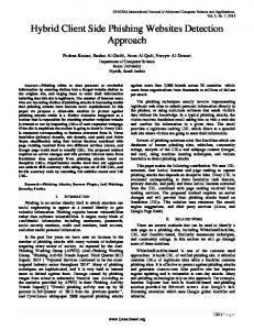
Figure 1. Outline of Fault-Proneness Filtering by Training only Errors
4.2. Training only errors In order to apply our approach to data from a source code repository, we implemented tools n m d “FPT in ” nd “FPCl ssifi ” fo aining and classifying software modules, respectively. The typical procedure for fault-proneness filtering is summarized as follows:
-3-
A Hybrid Fault-Proneness Detection Approach Using Text Filtering and Static Code Analysis Osamu Mizuno, Hideaki Hata
1. 2. 3. 4.
Apply FPClassifier to a newly created software module, Mi, and obtain the probability to be fault-proneness. By the threshold t FP (0 < t FP < 1), classify module Mi into FP or NFP. When the actual fault status (faulty or not-faulty) of Mi is revealed by a fault report, investigate whether the predicted result for Mi was correct or not. If the predicted result was correct, go to step 1; otherwise, apply FPTrainer to Mi to train each corpus and go to step 1.
This p o du is ll d h “T ining only o s (TOE)” p o du b us h ining process is invoked only when classification errors happen. The TOE procedure is quite similar to an actual classification procedure in practice. For example, in an actual e-mail filtering, email messages are classified when they arrive. If some of them are misclassified, each corpus (spam or ham) should be trained. Figure 1 shows an outline of this approach. At this point, we consider that fault -proneness filtering can be applied to the set of software modules developed in the same (or a similar) project. As referred to in [1], fault-prone codes could be spread also on different parts in a class file. We thus used class files of a Java program in each revision as a software module.
4.3. Static code analyzer: PMD PMD is an open source static analysis tool. PMD scans Java source code and looks for potential problems with particular rules. For example, with the unused code rule, it can check for unused fields and unused method parameters. With the basic rule, empty try/catch/finally/if/while blocks can be found. There are a lot of rules that cover various common issues in Java code. PMD reports each problem with its priority. Priorities are defined as follows: P1: Change absolutely required. Behavior is critically faulty. P2: Change highly recommended. Behavior is quite likely to be faulty. P3: Change recommended. Behavior is confusing, perhaps faulty. Priorities P4 and P5 are optional. In this study, we used PMD with following ten rules: r1: basic, r2: braces, r3: code size, r4: coupling, r5: design, r6: naming, r7: optimizations, r8: strict exception, r9: strings, r10: unused code.
4.4. A new approach Our new approach tries to decrease efforts to apply a static code analyzer. To do so, we propose the following procedure: 1. We apply the fault-proneness filtering to source code modules. We then obtain modules that are classified as fault-prone. 2. For fault-prone modules, we evaluate the severity of the module by applying the PMD with pre-selected rules. We can suggest that fault-prone modules with high priority should be removed immediately.
5. Implementation of Fault-proneness Filtering This section describes the implementations of fault-proneness filtering. To begin, we describe basic techniques of fault-proneness filtering based on our observations.
5.1. Observations and techniques 5.1.1. Precise training
-4-
International Journal of Advancements in Computing Technology Volume 2, Number 5, December 2010
In order to take into account of the difference between spam filtering and fault-proneness filtering, we observed training step and classification step. After that, we introduced two techniques, precise training and dynamic change of threshold. We observed that in fault-proneness filtering, there is only small difference between FP and NFP modules. This is because vocabulary is poorer in programming languages than in natural languages. In addition, most part of a module contains no features that distinguish faulty and non-faulty. A bug-introducing change is a modification that introduces bugs into the source code. If a module contains bug-introducing changes, we considered it a faulty module. However in such a faulty module, which we want to detect it is FP module, there must be not bug-introducing changes as well as bug-introducing changes. Because of this observation, we can conclude that we need a more precise training. That is, we need to train each corpus with only features that distinguish FP and NFP. So, we use parts of texts that contain some characterizing features. Only bug-introducing changes are stored in the fault corpus and only bug -fix changes that resolve bug modifications, are stored in the fix corpus. Such input of the FPTrainer allows a bigger difference between the corpora of fault and fix, because a bug-introducing change must not be in not-faulty modules, and a bug-fix change must not be in faulty modules that are related to the bug. 5.1.2. Dynamic change of threshold In spam filtering, if an e-mail message contains many features of ham, it should be classified into ham. However in fault-proneness filtering, if a module contains a bug-introducing change, we need to classify the module into FP even though it contains many features of non-faulty. Because of this observation, we need a more proper classification procedure. To this end, we introduce a dynamic threshold. That is, we change the threshold, after misclassification has happened because of a not proper threshold value. We guessed that the threshold varies depending on the characteristics of modules. We also guessed that more accurate classification might be obtained with the dynamic threshold. We thus define the way to change the threshold according to the types of modules. The way of changing the threshold is simple as follows: If an actual not-faulty module was misclassified as FP, then the threshold moves higher. That is, more modules are detected as NFP. If an actual faulty module was misclassified into NFP, then the threshold moves lower. That is, more modules are detected as FP. This is because we can avoid misclassification of not-faulty modules if the threshold is sufficiently high. Contrary to that, we can avoid misclassification of faulty modules if the threshold is sufficiently low.
5.2. Finding modified lines x
At first, we need to identify bug-introducing changes and bug-fix changes. These changes are d s h ng d lin s. W ll su h h ng s s “modifi d lin s”. In his p p , w ll
lines of bug-in odu ing h ng “f ul lin s”, nd lin s of bug fix h ng s “fix lin s”. A set of fault lines and fix lines can be extracted after one bug is resolved. We collect sets of fault lines and fix lines to train fault and fix corpora. Both fault lines and fix lines are extracted from source code repositories b s d on n lgo i hm p opos d by liw sski, Zimmermann, and Zeller (the SZZ algorithm) [24]. The following restriction and assumption exist in this collection method: Restriction: We seek fault lines and fix lines by examining CVS logs. Therefore, faults that do not appear in the CVS logs cannot be considered. That is, the set of FP modules used in this study is not complete. Assumption: We assume that faults are reported just after they are injected in the software.
-5-
A Hybrid Fault-Proneness Detection Approach Using Text Filtering and Static Code Analysis Osamu Mizuno, Hideaki Hata
Next, we collected the following information from a bug database of a target project such as Bugzilla. FLT : A set of faults found in a bug database. fi: Each fault in FLT. date(fi): Date in which a fault fi is reported. Here, we consider a line of source code Lj with dj, where dj is the last modified date of Lj. We then start mining a source code repository according to the following algorithm to extract fault lines and fix lines. 1. For each fault fi, find a certain revision of class CRFixedRev in which the fault has just been fixed by checking all revision logs. 2. Take the difference with each CRFixedRev and just previous revision of the same class. 3. For each line Lm in a CRFixedRev, Lm is a fix line if it is changed or added. 4. For each previous changing or deleting line Ln in the just previous revision class, examine dn, if dn < date(fi), Ln is a fault line. This algorithm collects a pair of fault lines and fix lines. An illustrated example of collecting fault lines and fix lines is shown in Figure 2. In this example, assume that the class that has the fixed revision classes CRFixedRev has revisions 1.1, 1.2, ..., 1.9, and revision logs are appended when each revision is committed. First, a fault f100 is found on 24th December, 2007. By searching all revision logs, assume that the fixed point is found at revision 1.9 of the class CRFixedRev (Shown as (1) in Figure 2). Then, take the difference between revision 1.8 and 1.9 (Shown as (2) in Figure 2). In the CRFixedRev, lines i and j are changed, and a line k is added, that is they are bug-fix change lines. So these 3 lines are fix lines. Lines a, g, and f in revision 1.8 of the class are prospective fault lines since changes or deletions occur in the next revision. In prospective fault lines, by searching revision differences, we find lines that have not been modified since the 24th of December, 2007. This is the purpose of removing prospective fault lines not being related to the f100. After checking the last modified date of each prospective fault line, lines a and f are accepted as fault lines, b ut line g is not. We implemented a prototype tool to track bugs in the CVS and Subversion repository. The inpu s of h ool CM sys m’s posi o y of h g p oj nd bug po o k. The outputs of the tool are sets of fault lines and fix lines.
Figure 2. Collection of fault and fix lines
-6-
International Journal of Advancements in Computing Technology Volume 2, Number 5, December 2010
6. Experiments 6.1. Target projects For the experiment, we selected open source software projects that can track faults. For this reason, we targeted three projects: Eclipse BIRT (BIRT), Groovy, a nd JRuby. Table1 shows the context of each target project. These projects are constructed in Java language, and revisions are maintained by CVS or Subversion. We also obtained a fault report from the bug database of each projects. We extracted faults from the bug database, Bugzilla or JIRA, under the following conditions: The type of these f ul s is “bugs”, h fo h s f ul s do no in lud ny nh n m n s o fun ion l p h s. Th s us of f ul s is “ solv d”, “v ifi d”, o “ los d”, nd h solu ion of f ul s is “fix d”. This means that the collected faults have already been fixed and been resolved, and thus fixed revision should be included in the entire repository. The severity of the faults was either blocker, critical, major, or normal, minor, trivial. Using our faulty modules collection tool, we collected both faulty and not -faulty modules from these three projects. The result of the collection is shown in Table 2.
Project (a) BIRT (b) Groovy (c) JRuby
Table 1. Target projects Size of repository (period) # of bug IDs (period) 685MB (01/2005-07/2008) 387MB (09/2003-07/2008) 68MB (09/2002-07/2008)
9,585 (02/2005-08/2008) 1,345 (10/2003-08/2008) 1,819 (07/2006-08/2008)
Table 2. Result of module collection for target projects Project Faulty modules Not-faulty modules (a) BIRT (b) Groovy (c) JRuby
23,947 2,494 7,680
32,600 8,827 5,586
6.2. Result of fault-proneness filtering For the evaluation of the experiments, we define several evaluation measures. Table 3 shows a legend of tables for experimental result. In Table 3, n1 shows the number of modules that are predicted as NFP, and are actually not-faulty modules. n2 shows the number of modules that are predicted as FP but are actually not-faulty modules. Usually, n2 is called a false positive. On the contrary, n3 shows the number of modules that are predicted as NFP, but are actually faulty modules. n3 is called a false negative. Finally, n 4 shows the number of modules that are predicted as FP and are actually faulty modules. Table 3. Legend of classification matrix Prediction NFP FP Actual
Not-faulty Faulty
n1 n3
n2 n4
For evaluation purposes, we used three measures: recall, precision, and F1. Recall is the ratio of modules correctly predicted as FP to the number of entire module s actually faulty. Recall is defined as follows: n4 recall n3 n4
-7-
A Hybrid Fault-Proneness Detection Approach Using Text Filtering and Static Code Analysis Osamu Mizuno, Hideaki Hata
Intuitively speaking, recall implies the reliability of the approach because a large recall denotes that actual FP modules can be covered by the predicted FP modules. Precision is th e ratio of modules correctly predicted as FP to the number of entire modules predicted as FP. Precision is defined as follows: n4 precision n2 n4 Intuitively speaking, precision implies the cost of the approach because a small precision requires much effort to find actual FP modules from the predicted FP modules. and precision. F1 is defined as follows: F1 is used to combine recall
F1
2 recall precision recall precision
In this definition, recall and precision are evenly weighted. Table 4 shows the detailed classification results for three projects at the final point of the TOE application. The evaluation measures at the end of the TOE procedure for each projects is shown in Table 5. As referred in [10], when ratio of faulty modules is low, like Groovy, recall, pre cision, and F1 are relatively low. Otherwise, if there are enough faulty modules (over 40 %), like BIRT and JRuby, recall, precision, and F1 are over 0.80. Table 4. Classification matrix in the TOE experiment (a) BIRT Prediction NFP FP Actual
Not-faulty Faulty
26,545 2,919
5,240 20,934
(b) Groovy Prediction Actual
Not-faulty Faulty
NFP
FP
8,000 872
661 1,622
(c) JRuby Prediction Actual
Not-faulty Faulty
NFP
FP
4,202
933
775
6,902
Table 5. Prediction accuracy in each project Project Recall Precision F1 (a) BIRT (b) Groovy (c) JRuby
0.878 0.650 0.899
0.800 0.710 0.881
0.837 0.679 0.890
Table 6. Target modules for PMD comparison Project # of modules Period (a) BIRT (b) Groovy (c) JRuby
1,282 1,197 1,112
6.3. Comparison with PMD
-8-
09/2007 – 10/2007 09/2007 – 12/2007 09/2007 – 10/2007
International Journal of Advancements in Computing Technology Volume 2, Number 5, December 2010
In order to compare fault-proneness filtering and PMD, we extract modules in three projects. Table 6 shows the number of modules and each extracted period. To compare with PMD, we have to investigate the output of PMD for each module manually. That is why we extracted about 1,000 modules from each project. We applied PMD of ten rules to these modules and compared the result of fault-proneness filtering. Table 7 shows the results of three projects. n1, n2, n3, and n4 are defined in subsection 6.2. n1 and n2 modules are not-faulty modules. n3 and n4 modules are faulty modules. Each row represents a category classified by fault-proneness filtering, and each number in each cell is the number of modules alerted by PMD. This means that PMD alerts with priorities, P1, P2, or P3. The ratio of alerted modules is shown in parentheses. Ratios larger than 50% are shown in bold.
Rules r1 r2 r3 r4 r5 r6 r7 r8 r9 r10
Rules r1 r2 r3 r4 r5 r6 r7 r8 r9 r10
Rules r1 r2 r3 r4 r5 r6 r7 r8 r9 r10
Table 7. Result of fault-proneness filtering and PMD (a) BIRT n1 = 441 n2 = 165 n3 = 68 78 (17.7%) 207 (46.9%) 160 (36.3%) 65 (14.7%) 300 (68.0%) 301 (68.3%) 389 (88.2%) 56 (12.7%) 73 (16.6%) 24 (5.4%)
n1 = 847 234 (27.6%) 382 (45.1%) 369 (43.6%) 130 (15.3%) 578 (68.2%) 636 (75.1%) 778 (91.9%) 181 (21.4%) 140 (16.5%) 215 (25.4%)
n1 = 228 28 (12.3%) 53 (23.2%) 77 (33.8%) 13 (5.7%) 124 (54.4%) 138 (60.5%) 189 (82.9%) 23 (10.1%) 40 (17.5%) 31 (13.6%)
66 (40.0%) 86 (52.1%) 77 (46.7%) 34 (20.6%) 128 (77.6%) 119 (72.1%) 151 (91.5%) 14 (8.5%) 32 (19.4%) 14 (8.5%)
(b) Groovy n2 = 96 53 (55.2%) 70 (72.9%) 61 (63.5%) 41 (57.8%) 77 (80.2%) 84 (87.5%) 92 (95.8%) 46 (47.9%) 39 (40.6%) 52 (54.2%)
(c) JRuby n2 = 99 40 (40.4%) 57 (57.6%) 66 (66.7%) 22 (22.2%) 89 (89.9%) 88 (88.9%) 96 (97.0%) 43 (43.4%) 59 (59.6%) 19 (19.2%)
34 (50.0%) 48 (70.6%) 41 (60.3%) 21 (30.9%) 62 (91.2%) 54 (79.4%) 68 (100%) 7 (10.3%) 17 (25.0%) 7 (10.3%)
n4 = 608 429 (70.6%) 456 (75.0%) 493 (81.1%) 341 (56.1%) 585 (96.2%) 561 (92.3%) 599 (98.5%) 88 (14.5%) 200 (32.9%) 169 (27.8%)
n3 = 152
n4 = 102
114 (75.0%) 146 (96.1%) 139 (91.4%) 73 (48.0%) 150 (98.7%) 151 (99.3%) 152 (100%) 65 (42.8%) 103 (67.8%) 63 (41.4%)
67 (65.7%) 87 (85.3%) 97 (95.1%) 59 (57.8%) 99 (97.1%) 102 (100%) 102 (100%) 64 (62.7%) 41 (40.2%) 26 (25.5%)
n3 = 61
n4 = 724
12 (19.7%) 28 (45.9%) 24 (39.3%) 8 (13.1%) 51 (83.6%) 55 (90.2%) 61 (100%) 7 (11.5%) 16 (26.2%) 13 (21.3%)
330 (45.6%) 546 (75.4%) 643 (88.8%) 258 (35.6%) 649 (89.6%) 708 (97.8%) 706 (97.5%) 194 (26.8%) 490 (67.7%) 231 (31.9%)
We can classify rules into three types as follows: 1. On rules, r5 (design), r6 (naming), and r7 (optimization), PMD alerts to most modules in all categories. This means that these rules cause false positives, that is, most alerts do not always cause faults. We classify them as the first type. For this type, we guess that false positives can be removed by combining fault-proneness filtering.
-9-
A Hybrid Fault-Proneness Detection Approach Using Text Filtering and Static Code Analysis Osamu Mizuno, Hideaki Hata
2. PMD with rules, r2 (braces) and r3 (code size), runs similarly to fault-proneness filtering. That is, PMD alerts to the most of same modules which fault -proneness filtering predicted as FP. We classify them as the second type. 3. PMD with the other rules, r1 (basic), r4 (coupling), r8 (strict exception), r9 (strings), and r10 (unused code) do not generate alerts much. We classify them as the third type.
6.4. A hybrid approach With the result of the comparison, we propose a hybrid fault -proneness detection approach using fault-proneness filtering and PMD. As shown in subsection 6.2, fault-proneness filtering could classify modules as fault-prone or not-fault-prone well. In order to see what kind of faults the modules predicted as fault -prone have, we apply PMD to them. As analyzed in subsection 6.3, there are three types of rules. First type rules cause high false positives, followed by second type, and third type. This means that third type rules are most significant, followed by second type, and first type. However, PMD with third type rules do not alert much. Therefore, if there are alerts of third type rules, we suggest their alerts to developers. If there is no alert of third type rules, but there are second type rules alerts, we suggest second type rules alerts. And if there is no alert of third or second type rules, but there are first type rules alerts, we suggest first type rules.
6.5. Threats to validity The threats to validity are categorized into 4 threats as recommended in [26]: external, internal, conclusion, and construction validity. In this study, t here are some threats to external and construction validity. One of the external validity threats for our study is the generality of target projects. We must study with more projects and analyze performance across them. In addition, industrial projects may lead to different results. Construction validity threats are identified as follows: The collection of faulty and not -faulty modules from open source software projects is incomplete. The algorithm adopted in this study has a limitation in that faults that are not recorded in a CVS log cannot be collected. To make an accurate collection of FP modules from source code repository, further research is required. The identification of faulty lines and fix lines is also incomplete. With the algorithm we adopt, there is incorrect identification of fault lines(bug-introducing lines) and fix lines(bug-fix lines).These incorrect identification and storing corpora may cause undesirable result. The identification algorithm depends on logs of projects. Therefore, if we ca nnot identify these lines sufficiently, fault-proneness filtering might work well. Smaller granularity of training units, modified lines of code, may be ignoring the context. That is, when certain lines are modified as bug-introducing lines, which may be completely different from another context where the same lines are changed but not introduce a bug. However, bigger granularity of training units may contain much noise. This is a trade-off problem.
7. Conclusion We proposed a hybrid fault-prone module detection method using fault-proneness filtering and a static code analyzer, PMD. Fault-proneness filtering can classify modules as fault-prone or not-fault-prone well. PMD reports rich contents of potential problems about source code modules. Our hybrid method is intended to make use of both merits of two approaches. With our hybrid method, we can reduce false positives and concentrate on significant PMD alerts.
8. Acknowledgements
- 10 -
International Journal of Advancements in Computing Technology Volume 2, Number 5, December 2010
This research is partially supported by the Japan Ministry of Education, Sc ience, Sports and Culture, Grant-in-Aid for Young Scientists (B), 20700025, 2010.
9. References [1] L. Aversano, L. Cerulo, and C. D. Grosso. Learning from bug-introducing changes to prevent fault prone code. In Ninth International Workshop on Principles of of w Evolu ion (IWP E’07), pages 19–26 2007. [2] V. R. Basili, L. C. Briand, and W. L. Melo. A validation of object oriented metrics as quality indicators. IEEE Trans. on Software Engineering, 22(10):751–761, 1996. [3] P. Bellini, I. Bruno, P. Nesi, and D. Rogai. Comparing fault-proneness estimation models. In Proc. of 10th IEEE International Conference on Engineering of Complex Computer Systems (ICECC ’05), p g s 205–214, 2005. [4] L. C. Briand, W. L. Melo, and J. Wust. Assessing the applicability of fault-proneness models across object-oriented software projects. IEEE Trans. on Software Engineering, 28(7):706–720, 2002. [5] G. Denaro and M. Pezze. An empirical evaluation of fault-proneness models. In Proc. of 24th International Conference on Software Engineering (IC E ’02), p g s 241–251, 2002. [6] N. E. Fenton and M. Neil. A critique of software defect prediction models. IEEE Trans. on Software Engineering, 25(5):675–689, 1999. [7] T. L. Graves, A. F. Karr, J. Marron, and H. Siy. Predicting fault incidence using software change history. IEEE Transactions on Software Engineering, 26(7):653–661, 2000. [8] L. Guo, B. Cukic, and H. Singh. Predicting fault prone modules by the dempster-shafer belief networks. In Proc. of 18th IEEE International Conference on Automated Software Engineering (A E’03), p g s 249–252, 2003. [9] A. E. Hassan and R. C. Holt. The top ten list: Dynamic fault prediction. In Proc. of the 21st IEEE In n ion l Conf n on of w M in n n (IC M’05), p g s 263–272, 2005. [10] H. Hata, O. Mizuno, and T. Kikuno. An extension of fault-prone filtering using precise training and dynamic threshold. In Proc. of 5th Working Conference on Mining Software Repositories (MSR2008), pages 89–97, May 2008. [11] T. M. Khoshgoftaar and N. Seliya. Comparative assessment of software quality classification techniques: An empirical study. Empirical Software Engineering, 9:229–257, 2004. [12] S. Kim, J. E. James Whitehead, and Y. Zhang. Classifying software changes: Clean or buggy? IEEE Transactions on Software Engineering, 34(2):181–196, March/April 2008. [13] S. Kim and M. D. Ernst. Which warnings should i fix first? In The 6th joint meeting of the European Software Engineering Conference and the ACM SIGSOFT Symposium on the Foundations of Software Engineering (ESEC/FSE2007), pages 45–54, 2007. [14] S. Kim, T. Zimmermann, E. J. W. Jr., and A. Zeller. Predicting faults from cached history. In Proc. of the 29th International Conference on Software Engineering (ICSE2007), pages 489–498, 2007. [15] J. Madhavan and E. Whitehead Jr. Predicting buggy changes inside an integrated development environment. Proc. of the 2007 OOPSLA workshop on eclipse technology eXchange, pages 36–40, 2007. [16] T. Menzies, J. Greenwald, and A. Frank. Data mining static code attributes to learn defect predictors. IEEE Trans. on Software Engineering, 33(1):2–13, January 2007. [17] O. Mizuno and T. Kikuno. Training on errors experiment to detect fault-prone software modules by spam filter. In The 6th joint meeting of the European Software Engineering Conference and the ACM SIGSOFT Symposium on the Foundations of Software Engineering (ESEC/FSE2007), pages 405–414, 2007. [18] J. C. Munson and T. M. Khoshgoftaar. The detection of fault-prone programs. IEEE Trans. on Software Engineering, 18(5):423–433, 1992. [19] N. Nagappan and T. Ball. Use of relative code churn measures to predict system defect density. In Proc. of the 27th International Conference on Software Engineering (ICSE2005), pages 284–292, 2005.
- 11 -
A Hybrid Fault-Proneness Detection Approach Using Text Filtering and Static Code Analysis Osamu Mizuno, Hideaki Hata
[20] S. Neuhaus, T. Zimmermann, C. Holler, and A. Zeller. Predicting vulnerable software components. In Proc. of h 14 h ACM Conf n on Compu nd Communi ions u i y (CC ’07), pages 529–540, 2007. [21] N. Rutar, C. B. Almazan, and J. S. Foster. A comparison of bug finding tools for java. In Proc. of the 15th International Symposium on Software Reliability Engineering (ISSRE2004), pages 245– 256, 2004. [22] A. h , T. Zimmermann, and A. Zeller. Predicting component failures at design time. In Proc. of the 2006 ACM/IEEE International Symposium on Empirical Software Engineering (ISESE06), pages 18–27, 2006. ACM. [23] N. Seliya, T. M. Khoshgoftaar, and S. Zhong. Analyzing software quality with limited faultproneness defect data. In Proc. of Ninth IEEE International Symposium on High-Assurance ys ms Engin ing (HA E’05), p g s 89–98, 2005. [24] J. liw ski, T. Zimmermann, and A. Zeller. When do changes induce fixes? (on Fridays.). In Proc. of 2nd International Workshop on Mining Software Repositories (MSR2005), pages 24–28, 2005. [25] M. Stoerzer, B. G. Ryder, X. Ren, and F. Tip. Finding failure-inducing changes in java programs using change classification. In Proc. of 14th ACM SIGSOFT International Symposium on Foundations of Software Engineering (FSE2006), pages 57–68, 2006. [26] C. Wohlin, P. Run son, M. H s , M. C. Ohlsson, . R gn ll, nd A. W ssl n. Experimentation in software engineering: An introduction. Kluwer Academic Publishers, 2000.
- 12 -