A Hybrid Framework for Image Segmentation Using ... - CiteSeerX

A Hybrid Framework for Image Segmentation Using Probabilistic Integration of Heterogeneous Constraints Rui Huang, Vladimir Pavlovic, and Dimitris N. Metaxas Department of Computer Science, Rutgers University, Piscataway, NJ 08854 {ruihuang,vladimir,dnm}@cs.rutgers.edu Abstract. In this paper we present a new framework for image segmentation using probabilistic multinets. We apply this framework to integration of regionbased and contour-based segmentation constraints. A graphical model is constructed to represent the relationship of the observed image pixels, the region labels and the underlying object contour. We then formulate the problem of image segmentation as the one of joint region-contour inference and learning in the graphical model. The joint inference problem is solved approximately in a band area around the estimated contour. Parameters of the model are learned on-line. The fully probabilistic nature of the model allows us to study the utility of different inference methods and schedules. Experimental results show that our new hybrid method outperforms methods that use homogeneous constraints.

1 INTRODUCTION Image segmentation is an example of a challenging clustering/classification problem where image pixels are grouped according to some notion of homogeneity such as intensity, texture, color, motion layers, etc. Unlike many traditional clustering/classification problems, where the class labels of different query points are inferred independently, image segmentation can be viewed as a constrained clustering/classification problem. It is reasonable to expect that class-labels of points that are in spatial proximity of each other will be similar. Moreover, the boundaries of segmented image regions are often smooth, imposing another constraint on the clustering/classification solution. Markov Random Fields (MRFs) have long been used, with various inference techniques, in image analysis, because of their ability to impose the similarity constraints among neighboring image pixels and deal with the noise [1–5]. The MRF-based image segmentation method is an important representative of region-based segmentations, which assign image pixels to a region according to some image property (e.g., region homogeneity). The other major class of image segmentation methods are edge-based segmentations, which generate boundaries of the segmented objects. Among others, deformable models and their variants [6–9] are important representatives of this class. Though one can label regions according to edges or detect edges from regions, the two kinds of methods are naturally different and have respective advantages and disadvantages. The MRF-based methods work well in noisy images, where edges are usually difficult to detect while the region homogeneity is preserved. The disadvantages of these methods are that they may generate rough edges and holes inside the objects, and they do not take account of the shape and topology of the segmented objects. On the other hand, in deformable model-based methods, a prior knowledge of object shape can be

easily incorporated to constrain the segmentation result. While this often leads to sufficiently smooth boundaries, the oversmoothing may be excessive. And these methods rely on edge detecting operators, so they are sensitive to image noise and may need to be initialized close to the actual region boundaries. The real world images, especially medical images, usually have significant, often non-white noise and contain complex high-curvature objects with a strong shape prior, suggesting a hybrid method to take advantages of both MRFs and deformable models. In this paper we propose a fully probabilistic graphical model-based framework to combine the heterogeneous constraints imposed by MRFs and deformable models, thus constraining the image segmentation problem. To tightly couple the two models, we construct a graphical model to represent the relationship of the observed image pixels, the true region labels and the underlying object contour. Unlike traditional graphical models, the links between contour and region nodes are not fixed; rather, they vary according to the state (position) of the contour nodes. This leads to a novel representation similar to Bayesian multinets [10]. We then formulate the problem of image segmentation under heterogeneous constraints as the one of joint region-contour inference and learning in the graphical model. Because the model is fully probabilistic, we are able to use the general tools of probabilistic inference to solve the segmentation problem. We solve this problem in a computationally efficient manner using approximate inference in a band area around the estimated contour. The rest of this paper is organized as follows: section 2 reviews the previous work; section 3 introduces a new integrated model; detailed inference on the coupled model is described in section 4; section 5 shows the experimental results and comparison of alternative inference methods and schedules; and section 6 summarizes the paper and future work.

2 PREVIOUS WORK Because the exact MAP inference in MRF models is computationally infeasible, various techniques for approximating the MAP estimation have been proposed, such as MCMC [1], ICM [2], MPM [3], and two of the more recently developed fast algorithms: Belief Propagation (BP) [4] and Graph Cuts [5]. The estimation of the MRF parameters is often solved using the EM algorithm [11]. However, MRFs do not take account of object shape and may generate rough edges and even holes inside the objects. Since the introduction of Snakes [6], variants of deformable models have been proposed to address problems such as initialization (Balloons [7] and GVF Snakes [9]) and changes in model’s topology [8]. One limitation of the deformable model-based method is its sensitivity to image noise, a common drawback of edge-based methods. Methods for integration of region and contour models were studied in [12, 13] using inside-outside and stochastic Gibbs models. The joint contour-region inference is accomplished using general energy minimization methods, without explicit model parameter learning. Chen et al. proposed a way of integrating MRFs and deformable models in [14] using a loosely coupled combination of MRFs and balloon models. [15] first introduced a more tightly coupled MRF-balloon hybrid model. While the model employs a probabilistic MRF, it still relies on a traditional energy-based balloon inference. The model we propose in this paper differs because it is fully probabilistic, in both the

region and the contour constraints. This unified framework allows for probabilistic inference and machine learning techniques to be applied consistently throughout the full model, and not only to some of its parts, as in [15]. This allows us to systematically study the utility of different inference methods and schedules. Moreover, our formulation opens up the possibility to easily impose more specific constraints, such as the shape priors, by appropriately settings the model’s parameters (or their priors).

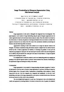
3 INTEGRATED MODEL The integrated MRF-contour model structure is depicted in Fig. 1(a). yi y (image pixels)

pi ( si ) di-1

d i ' +1 ( x d i ' +1 , y d i ' +1 )

ci-1

s (region labels)

sign = '+ '

di

sign = '− '

loc(i ) = ( xi , yi )

ci

di ' ( xdi ' , ydi ' )

c (underlying contour)

(a) Integrated model

|d|

ci ' di+1

(b) Contour

(c) Signed distance

mij ( s j )

si

p ij ( si , s j )

mi ' i ( si )

pii ' ( si , ci ' )

m ii ' ( c i ' )

p i ' j ' ( ci ' , c j ' ) c i '

mi' j' (c j' )

pi ' ( ci ' )

(d) BP Rules

Fig. 1. Structure and definition of the integrated model.

The model consists of three layers: the image pixel layer, the region label layer, and the contour layer. Let n be the number of pixels in the image. A configuration of the observable layer is y = (y1 , ..., yn ), yi ∈ D, i = 1, ..., n, where D is a set of pixel values, e.g., gray values 0-255. Similarly, a configuration of the hidden layer is s = (s1 , ..., sn ), si ∈ L, i = 1, ..., n, where L is a set of region labels, such as L = {inside, outside}. The contour representation c (Fig. 1(b)) is slightly different from the traditional representations used in energy-based models. Let d = (d1 , ..., dm ) be the m contour node positions di = (xdi , ydi ) in the image plane. We define c = (c1 , ..., cm ) as ci = (di , di+1 ), i = 1, ..., m − 1, cm = (dm , d1 ). That is, each node ci in our model is a segment of the actual contour. The edges between the s layer and the c layer are determined based on the distance between the image pixels and the contour segments: each pixel label node si is connected to its nearest contour segment ci0 i ← i0 = arg min dist(i, cj ). j

Hence, the graph structure depends on the state of the contour nodes ci0 . A model of this type is often referred to as a multinet [10]. The segmentation problem can now be viewed as a joint MAP estimation problem: (c, s, θ)M AP = arg max P (c, s, θ|y)

(1)

P (c, s, θ|y) ∝ P (y|s, θ)P (s, c|θ)P (θ).

(2)

c,s,θ

where

Note that we include the estimation of model parameters θ as a part of the segmentation process. To define the joint distribution of the integrated model, we model the image likelihood term P (y|s) identical to the traditional MRF model (we drop the dependency on parameters θ when obvious): ¶ µ Y Y Y (yi − µsi )2 1 p exp − (3) P (y|s) = P (yi |si ) = pi (si ) = 2 i

i

2σsi

2πσs2i

i

where we assume the image pixels are corrupted by white Gaussian noise. The second term P (s, c) models a joint distribution of region labels and the contour. We represent this distribution in terms of two compatibility functions, rather than probabilities: P (s, c) =

1 Ψsc (s, c)Ψc (c). Z(s, c)

(4)

The first term models the compatibility of the region labels with the contour, defined as: Q Q Ψsc (s, c) =

=

ψij (si , sj )

(i,j)

=

Ψsc (si , ci0 )

Ψss (si , sj )

Q

(i,j)

Q i

exp

³

i Q

i δ(si −sj ) σ2

ψii0 (si , ci0 )

´Q

(5)

ψii0 (si , ci0 )

i

where we incorporated a shape c to constrain the region labels s, in addition to the original Gibbs distribution. Note that the dependency between the contour and the region labels is not deterministic. The uncertainty in region labels for a given contour can arise as an attempt to model, e.g., image aliasing and changes in region appearance at boundaries. Since we only segment one specific region at a time, we need only consider the pixels near the contour, and label them either inside or outside the contour. We model the dependency between the contour c and the region labels s using the softmax function: ¡ ¢ (s) ψii0 (si = inside, ci0 ) ∼ 1/ 1 + exp(−d

(i, ci0 ))

(6)

induced by the signed distance of pixel i from the contour segment ci0 (see Fig. 1(c)): d(s) (i, ci0 ) = (di0 − loc(i)) × (di0 +1 − di0 )/|di0 +1 − di0 |

(7)

where loc(i) denotes the spatial coordinates of pixel i. This equation only holds when the pixel is close to the contour, which accords with our assumption. When the contour nodes are ordered counter-clockwise, the sign is positive when pixel i is inside the contour and negative when it is outside. The contour prior term P (c) can be represented as: Y Y Y Y Ψc (c) =

Ψcc (ci0 −1 , ci0 )

i0

Ψb (ci0 ) =

i0

ψi0 −1,i0 (ci0 −1 , ci0 )

(i0 −1,i0 )

ψi0 (ci0 )

(8)

i0

where ψi0 −1,i0 (ci0 −1 , ci0 ) is the contour smoothness term and ψi0 (ci0 ) is used to simulate the balloon force.

Despite the compact graphical representation of the integrated model, the exact inference in the model is computationally intractable. One reason for this is the large state space size of the contour nodes (the 2D image plane). To deal with this problem we restrict the contour searching to a set of normal lines along the current contour, as proposed in [16] (see Fig. 1(b)). That is, the state space of each contour node di is restricted to a small number, e.g., k, distinct values. In turn, the state space of each contour segment ci is of size k 2 . Now we can easily calculate the discretized contour smoothness term: ³ ´ |d −d |2 |d +d −2d |2 ψi0 −1,i0 (ci0 −1 , ci0 ) = e

−ω1

i0 −1 i0 +1 4h2

−ω2

i0 −1

i0 +1 h4

i0

(9)

and simulate the balloon force by defining ψi0 (ci0 ) = [ψi0 ,1 , ..., ψi0 ,k ], where ψi0 ,j is the prior of each state j at the contour node di0 . Lastly, the parameter priors P (θ) are chosen from the appropriate conjugate prior families and are assumed to be uninformative. In this paper we primarily focus on the MRF parameters.

4 MODEL INFERENCE USING BP The whole inference/learning algorithm for the hybrid model can now be summarized as below. The goal of our segmentation method is to find one specific region with a smooth and closed boundary. A seed point is arbitrarily specified and the region containing it is then segmented automatically. Thus, without significant loss of modeling generality, we simplify the MRF model and avoid possible problems caused by segmenting multiple regions simultaneously. Initialize contour c; while (error > maxError) { 1. Calculate a band area B around c. Perform remaining steps inside B; 2. Build links between the s and c layers according to the signed distances; 3. Calculate the discretized states at each contour node along its normal; 4. Estimate the MAP solution (c, s)M AP using BP with schedule S; 5. Update model parameters θM AP and contour position dM AP ; } As mentioned previously, the exact MAP inference even in the MRF model alone is often computationally infeasible. In our significantly more complex but probabilistic model, we resort to using the BP algorithm. BP is an inference method proposed by Pearl [17] to efficiently estimate Bayesian beliefs in the network by the way of iteratively passing messages between neighbors. It is an exact inference method in the network without loops. Even in the network with loops, the method often leads to good approximate and tractable solutions [18]. The implementation of BP in our model is slightly more difficult than the BP algorithm in a traditional pairwise MRF, since the model structure is more complicated. One can solve this by converting the model into an equivalent factor graph, and use the BP algorithm for factor graphs [19, 20]. Here we give the straightforward algorithm for our specific model. Examples of the message passing rules are

 Y

mij (sj ) = max [ψi (si ) si

 mi0 i (si ) = max ψi0 (ci0 ) ci0

mki (si )mi0 i (si )ψij (si , sj )

k∈ℵ(i)\j

Y

(10)



mk0 i0 (ci0 )

k0 ∈ℵ(i0 )

Y

mki0 (ci0 )ψii0 (si , ci0 )

(11)

k∈ℵ0 (i0 )\i

with message definition given in Fig. 1(d). ℵ denotes the set of neighbors from the same layer, and ℵ0 denotes the set of neighbors from a different layer. The rules are based on the max-product scheme. At convergence, the beliefs, e.g., of the pixel labels are Q bi (si ) ∼ ψi (si )

k∈ℵ(i)

mki (si )mi0 i (si ).

(12)

A crucial question in this BP process is that of the “right” message passing schedule [19, 20]. Different schedules may result in different stable/unstable configurations. For instance, it is widely accepted that short graph cycles deteriorate the performance of the BP algorithm. We empirically study this question in Section 5.3 and show that good schedules arise from understanding of the physical processes involved. The BP is evoked only in a band area around current contour. A primary reason for the band-limited BP update is the computational complexity of inference. Moreover, the band-limited update can also be justified by the fact that the region labels of pixels far from the current contour have little influence on the contour estimates. When the BP algorithm converges, the model parameters (i.e., µsi and σsi ) can be updated using following equations: X X X X 2 2 µl =

b(si = l)yi /

i

b(si = l), σl =

i

b(si = l)(yi − µl ) /

i

b(si = l)

(13)

i

where l ∈ {inside, outside} and b(·) denotes the current belief. Because the edges between the s layer and the c layer are determined by the distance between pixels and contour nodes, they also need to be updated in the inference process. This step follows directly after the MAP estimation.

5 EXPERIMENTS Our algorithm was implemented in MATLAB/C, and all the experiments were tested on a 1.5GHz P4 Computer. Most of the experiments took several minutes on the images of size 128×128. 5.1 COMPARISON WITH OTHER METHODS The initial study of properties and utility of our method was conducted on a set of synthetic images. The 64×64 perfect images contain only 2 gray levels representing the ”object” (gray level is 160) and the ”background” (gray level is 100) respectively. We then made the background more complicated by introducing a gray level gradient from 100 to 160, along the normal direction of the object contour to the image boundary (Fig. 2(a)). Fig. 2(b) shows the result of a traditional MRF-based method. The object is segmented correctly, however some regions in the background are misclassified. On the other hand, the deformable model slightly leaked from the high-curvature part of the

object contour, where the gradient in the normal direction is too weak (Fig. 2(c)). Our hybrid method, shown in Fig. 2(d), results in a significantly improved segmentation. We next generated a test image (Fig. 2(e)) by adding zero-mean Gaussian noise with σ 60 to Fig. 2(a). The result of the MRF-based method on the noisy image (Fig. 2(f)) is somewhat similar to that in Fig. 2(b), which shows the MRF can deal with image noise to some extent. But significant misclassification occurred because of the complicated background and noise levels. The deformable model either sticks to spurious edges caused by image noise or leaks (Fig. 2(g)) because of the weakness of the true edges. Unlike the two independent methods, our hybrid algorithm, depicted in Fig. 2(h), correctly identifies the object boundaries despite the excessive image noise. For visualization purposes we superimpose the contour on the original image (Fig. 2(a)) to show the quality of the result in Fig. 2(g) and Fig. 2(h).

(a) Input

(b) MRF

(c) DM

(d) GM

(e) Noisy

(f) MRF

(g) DM

(h) GM

Fig. 2. Experiments on synthetic images

(a)

(b)

(c)

(d)

Fig. 3. Experiments on medical images

Experiments with synthetic images outlined some of the benefits of our hybrid method. The real world images (e.g., medical images) usually have significant, often non-white noise and contain multiple regions and objects, rendering the segmentation task a great deal more difficult. Fig. 3(a) is a good example of difficult images with complicated global properties, requiring the MRF-based method to automatically determine the number of regions and the initial values of the parameters. Fig. 3(b) is obtained by manually specifying the inside/outside regions to get an initial guess of the parameters for the MRF model. Our method avoids this problem by creating and updating an MRF model locally and incrementally. Another problem with MRF-based method is that we can not get a good representation of the segmented object directly from the model. The image is also difficult for deformable models because the boundaries of the objects to be segmented have many high-curvature parts. Fig. 3(c) exemplifies the over-smoothed deformable models. Our method’s results, shown in Fig. 3(d) does not suffer from the problems. For the deformable model method, we started the balloon model at several different initial positions and use the best results for the comparison. On the other hand, our hybrid method is significantly less sensitive to the initialization of the parameters and the initial seed position.

5.2 COMPARISON OF DIFFERENT INFERENCE METHODS We compared our proposed inference method (MAP by BP) with three other similar methods: maximum marginal posterior (MM), iterative conditional modes (ICM), and Gibbs sampling. In the MM method the inference process is accomplished using the sum-product belief propagation algorithm [20]. The algorithm yields approximate marginal posteriors, e.g., P (si |y) that are then maximized on individual basis, e.g., si ∗ = arg maxsi P (si |y). The ICM and Gibbs inference methods, respectively, maximize and sample from the local conditional models, e.g., si ∗ = arg maxsi P (si |Markov Blanket(si )), one variable at a time.

−7000

−7500

−8000

Log Likelihood

−8500

−9000 SumProd −9500

MaxProd ICM

−10000

Gibbs −10500

−11000

−11500

0

5

10

15

20

25 Iteration

30

35

40

45

50

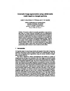
Fig. 4. Top: Final segmentation results of different inference schemes: (a) sum-product, (b) maxproduct, (c) ICM in MRF, sum-product in DM, and (d) Gibbs in MRF, sum-product in DM. Bottom: Changes in log likelihood during iterations of different inference schemes.

In all our experiments there was no substantial visible difference between the segmentation results of MAP and MM estimates, as exemplified by Fig. 4. Comparison of log likelihood profiles during inference revealed small differences—as expected, the sum-product inference outperforms the max-product in noisy situations. On the other hand, the use of ICM and Gibbs inference resulted in significantly worse final segmentation. For instance, when used only in the MRF layer, ICM and Gibbs-driven segmentation lead to final estimates shown in Fig. 4c and Fig.4d. Surprisingly, the differences in the log likelihood estimates appear to be less indicative of this final performance. The use of the two approximate inference methods, not shown here, in the DM layer resulted in very poor segmentation. 5.3 COMPARISON OF DIFFERENT MESSAGE PASSING SCHEDULES The choice of the message passing schedule in the BP algorithm is an interesting and still open problem. We experimented with two different schedules. In the first schedule S1 we first update messages mij (sj ) in s-layer until convergence (this usually takes two or three iterations in our experiments), and then send messages mii0 (ci0 ) once (which is essentially passing messages from s-layer to c-layer). Next, we update messages mi0 j 0 (cj 0 ) in c-layer until convergence (usually in one or two iterations), and finally update messages mi0 i (xi ), i.e., send messages back from c-layer to s-layer. In the other schedule S2 we started from the top of the model, update all the messages mij (sj ),

mii0 (ci0 ), mi0 j 0 (cj 0 ), and mi0 i (si ) in this sequence exactly once and repeat, until convergence. The two message passing schedules were chosen to study the importance of withinmodel (e.g., inside MRF) local consistency (schedule S1 ) and between-models local consistency (S2 ). The former message passing schedule may be intuitively more appealing considering the physical difference of the two models (MRFs and deformable models) we are coupling. Traditional energy-based methods also point in the direction of this schedule; integration of forces is usually first computed in the individual horizontal layers. Moreover, S1 leads to better experimental results. The upper two rows of Fig. 5 show, visually, the segmentation performance of the two schedules. The estimates of the likelihood resulting from the two schedule, displayed in the bottom row of Fig. 5, also indicate that S1 is preferred to S2 . Again, the contour is superimpose on the perfect image for visualization purposes.

Fig. 5. Experiments with different message passing schedule. Top: S1 , Center: S2 , Bottom: Log likelihoods (computed at MAP estimates) using the two different schedules.

6 CONCLUSIONS We proposed a new, fully probabilistic framework to combine two heterogeneous constraints, MRFs and deformable models, for the clustering/classification task of image segmentation. The framework was developed under the auspices of the probabilistic multinet model theory allowing us to employ a well-founded set of statistical estimation and learning techniques. In particular, we employed an approximate, computationally efficient solution to the otherwise intractable constrained inference of image regions. We showed the utility of our hybrid method and different inference schemes. We also presented two different message passing schedules. Finally, we point to the central role of inference schemes and message passing schedules in the segmentation process. We are now working on including a stronger shape prior to the model, in additional to current smoothness term and balloon forces. In our future work we will consider

similarity as well as dissimilarity constraints, specified by users or learned from data, to further reduce the feasible solution spaces in the context of image segmentation.

References 1. S. Geman and D. Geman. Stochastic Relaxation, Gibbs Distributions and the Bayesian Restoration of Images. IEEE Transaction on Pattern Analysis and Machine Intelligence, 6(6), 1984. 2. J. E. Besag. On the Statistical Analysis of Dirty Pictures. Journal of the Royal Statistical Society B, 48(3), 1986. 3. J. Marroquin, S. Mitter, and T. Poggio. Probabilistic Solution of Ill-posed Problems in Computational Vision. Journal of American Statistical Association, 82(397), 1987. 4. W.T. Freeman, E.C. Pasztor, and O.T. Carmichael. Learning Low-Level Vision. International Journal of Computer Vision, 40(1), 2000. 5. Y.Y. Boykov and M.P. Jolly. Interactive Graph Cuts for Optimal Boundary & Region Segmentation of Objects in N-D Images. Proceedings of ICCV, 2001. 6. M. Kass, A. Witkin, and D. Terzopoulos. Snakes: Active contour models. International Journal of Computer Vision, 1(4), 1987. 7. L.D. Cohen. On Active Contour Models and Balloons. Computer Vision, Graphics, and Image Processing: Image Understanding, 53(2), 1991. 8. T. McInerney and D. Terzopoulos. Topologically Adaptable Snakes. Proceedings of ICCV, 1995. 9. C. Xu and J.L. Prince. Gradient Vector Flow: A New External Force for Snakes. Proceedings of CVPR, 1997. 10. D. Geiger and D. Heckerman, Knowledge representation and inference in similarity networks and Bayesian multinets, Artificial Intelligence, 82:45-74, 1996. 11. Y. Zhang, M. Brady, and S. Smith. Segmentation of Brain MR Images Through a Hidden Markov Random Field Model and the Expectation-Maximization Algorithm. IEEE Transaction on Medical Imaging, 20(1), 2001. 12. U. Grenander and M. Miller. Representations of Knowledge in Complex Systems. Journal of the Royal Statistical Society B, 56(4), 1994. 13. S.C. Zhu and A.L. Yuille. Region Competition: Unifying Snakes, Region Growing, and Bayes/MDL for Multiband Image Segmentation. IEEE Transaction on Pattern Analysis and Machine Intelligence, 18(9), 1996. 14. T. Chen, D.N. Metaxas. Image Segmentation Based on the Integration of Markov Random Fields and Deformable Models. Proceedings of MICCAI, 2000. 15. R. Huang, V. Pavlovic, and D.N. Metaxas. A Graphical Model Framework for Coupling MRFs and Deformable Models. Proceedings of CVPR, 2004. 16. Y. Chen, Y. Rui, and T.S. Huang. JPDAF Based HMM for Real-Time Contour Tracking. Proceedings of CVPR, 2001. 17. J. Pearl, Probabilistic Reasoning in Intelligent Systems: Networks of Plausible Inference, Morgan Kaufmann Publishers, 1988. 18. Y. Weiss. Belief Propagation and Revision in Networks with Loops. Technical Report MIT A.I. Memo 1616, 1998. 19. F.R. Kschischang, B.J. Frey, and Hans-Andrea Loeliger. Factor Graphs and the Sum-Product Algorithm. IEEE Transactions on Information Theory, 47(2), 2001. 20. J.S. Yedidia, W.T. Freeman, and Y. Weiss. Understanding Belief Propagation and Its Generalizations. IJCAI 2001 Distinguished Lecture track, 2001