A hybrid heuristic algorithm for the no-wait flowshop ... - IEEE Xplore

A hybrid heuristic algorithm for the no-wait flowshop scheduling problem Vahid Riahi

Morteza Kazemi

Industrial Engineering Department Shiraz University of Technology Shiraz, Iran [email protected]

Industrial Engineering Department Shiraz University of Technology Shiraz, Iran [email protected]

Abstract— the no-wait flowshop scheduling problem (NWFSP) that needs jobs to be processed without interruption between consecutive machines is a NP-hard combinatorial optimization problem, and embodies a significant area in production scheduling. The objective is set to find the scheduling which minimizes the makespan. In this paper, a new hybrid ant colony optimization (ACO) and Simulated Annealing (SA) algorithm is presented to solve NWFSP. The computational results on 29 benchmark instances provided by Carlier and Reeves and comparison with other reported results in the literature approves the efficiency of the proposed algorithm. Keywords— no-wait flowshop scheduling; ant colony optimization; Simulated Annealing; maximum completion time

I. INTRODUCTION Scheduling is an important part of manufacturing systems. Flowshop scheduling problems have an extensive background in industrial applications, including steel production, mining, logistics, chemical industry and food processing. A comprehensive survey on the research and application of nowait flowshop scheduling problem can be found in Hall and Sriskandarayah’s review paper [1]. The general assumption of majority of flowshop applications is the sequencing of the jobs relies on buffers, otherwise they are considered as intermediate storage between machines. The no-wait flowshop scheduling problem (NWFSP) with makespan criterion is considered in this paper. In NWFSP, each job has to be processed from the first machine to the last one without any interruption and the job sequence is unique on all machines. In addition, each machine can handle no more than one job at a time and each job has to visit each machine exactly once. Therefore, the start of a job on the first machine may be delayed in order to meet the no-wait requirement. Given that the release time of all jobs is zero and set-up time on each machine is included in the processing time, the no-wait flowshop problem is to schedule jobs that minimize the makespan over all jobs. According to Garey and Johnson’s research work [2], the no-wait flowshop scheduling problem is NP-hard. In the operations research literature, many elegant mathematical models and solution methods have been developed to cope with real-world problems. Some exact approaches have been proposed to solve the problems optimally, but with the limitations of solving with only small-sized problems.

978-1-4673-9181-8/15/$31.00 ©2015 IEEE

On the other hand, heuristics are based on polynomial time algorithms and they are the most suitable methods to solve large scheduling problems. In general, heuristics yield good and satisfactory (but not necessarily global optimal) solutions in reasonable time [3] . Recently, local search-based methods, including simulated annealing Algorithm [4], Tabu Search algorithm [5], Variable Neighborhood Search [6] and metaheuristics with techniques such as genetic algorithm [7], ant colony algorithm [8], and particle swarm optimization [9] for the considered case have been developed. The ant colony algorithm was first proposed by Colorni, Dorigo, and Maniezzo [10] and has received extensive attention due to its successful applications to many combinatorial optimization problems [11]. For ACO applications in flowshop scheduling, Stutzle [12] applied the max–min ant system (MMAS), proposed by Stutzle and Hoos [13], to the flowshop scheduling problem for minimizing the makespan. Simulated Annealing (SA), is one of the most popular meta-heuristics for addressing combinatorial optimization problems over the past two decades. SA is a neighborhood search technique which lead to achievement of good results for combinatorial problems. Complete overviews of SA’s theoretical and applied developments can be found in Eglese [14]. It has been widely used to solve scheduling problems [15,16,17]. In the current study, the performances of hybrid ant colony optimization (ACO) and simulated annealing to solve the nowait flowshop scheduling problem with the objective of minimizing makespan will be investigated. Indeed, NWFSP has solved by ACO in previous works, however because of local optimum there were some undesired results or situations, so in order to improve results it is required to avoid local optimum, one way of avoiding local optimum is SA algorithm that we want to use it. The rest of the paper is organizes as follows: in section 2 the problem definition is presented. The framework of the proposed algorithm is discussed in section 3. Computational results and conclusions are come in section 4 and 5 respectively. II. THE NO-WAIT FLOWSHOP SCHEDULING PROBLEM The NWFSP can be defined as: a set of jobs are available for processing on machines. Each job has a sequence of operations. Each machine can process one job at a time and

each job must be performed only on one machine at a time. All jobs must be completed without interruption and the jobs should not wait to be scheduled between two successive machines. The problem is finding a schedule in a way that the processing order of jobs is the same on each machine and the maximum completion time is minimized.

1) Pheromone initialization Like PACO proposed by Rajendran and Ziegler [18], an initial differential setting of the trail intensities is considered. In

The following notations are used to formulate the no-wait flowshop problems:

the trail pheromone that calculated by the following formulas:

n

:

number of jobs to be scheduled,

m

:

number of machines in the no-wait flowshop,

ti,j

:

processing time for the ith job on the jth machine,

dj,k

:

minimum delay on the first machine between the start of job j and job k due to the no-wait

[i]

:

the job processed in position i,

C[i]

:

the completion time of the job processed in position.

The minimum delay time dj,k and completion time C[i] can be calculated using the following equations: j

j −1

p=2

p =1

di ,k = ti ,1 + max 2≤ j ≤ m (∑ tip − ∑ tkp , 0) m

C[1] = ∑ t[1], j j =1

C[ i ] =

i

∑d k =2

m

[ k −1],[ k ]

+ ∑ t[ i ], j j =1

III. DESCRIPTION OF THE PROPOSED ACO ALGORITHM In this section, we described the proposed hybrid ACO-SA algorithm for the no-wait flowshop scheduling problem. The ACO algorithm is utilized generate initial scheduling. Then the ACO solutions are improved by using SA method. The explanations of these algorithms are as follows: A. the proposed ACO algorithm The ACO meta-heuristic algorithm, was introduced by Colorni, et al. [9] for the first time, and has been successfully applied to a large number of combinatorial optimization problems. This algorithm is inspired by the behavior of real ants in finding the shortest path from a food source to the nest. In ACO algorithm a feasible solution is usually shown as a path in a graph. In NWFSP, the graph of the problem is shown with a complete graph where the vertices are corresponded to the activities. Each sequence for scheduling the jobs can be shown as a directed path which includes all the vertices in the graph of the problem. Therefore finding a feasible solution leads to finding such directed path.

τ ij

is considered as the intensity of assigning jth job in ith position. This desirability is changed during the running of the ACO algorithm. The main steps of the proposed algorithm for the NWFSP are as follows:

this paper, we consider an upper bound

τ min for

τ max and a lower bound

τ max = ((1 − ρ ) Z best ) −1

τ min = 0.2τ max where Z best denotes the best makespan obtained so far and ρ (0 ≤ ρ ≤ 1) is the parameter of the algorithm and for initially, it equals the makespan of Rajendran’s heuristic [19], so, the initial pheromone are chosen as τ ij = τ max = ((1 − ρ ) Z raj ) −1 for all i and j. 2) Make feasible solution To construct a job sequence, each artificial ant, k, is starting with an empty sequence, then iteratively adding a new job to its path, from the set of jobs has not yet selected, N kj , by using a state transition rule, so-called pseudo-random proportional rule [19] as follows: Ant k at the current position i, generates a random number q between 0 and 1. If q ≤ q0 , where q0 is the parameter of the algorithm, then the job with maximum pheromone trail in N kj will be selected. Otherwise job j in the position i from N kj will be selected by the probability of:

Pijk =

τ ij , i ∈ N kj ∑ τ ij

j∈ N kj

3) Local update of pheromone trail: To avoid premature convergence, a local trail update is performed. The local update reduces the pheromone amount of a new component so that the following ants have less probability to choose this job for the same place. This is achieved by the following local updating rule:

τ ijnew = ρτ ijold Where ρ (0 ≤

ρ ≤ 1)

is the parameter of the algorithm.

4) Global update of pheromone trail: The global updating rule is applied after all ants generate their solutions. The pheromone trails are modified according to the following global updating rule to make the search more directed:

τ ijnew

Zρ ⎧ old ρτ + ij k − best ⎪ c max =⎨ ⎪ ρτ old ⎩ ij

if job j is placed in position i in the best solution found so far Otherwise

where 0 ≤

After modifying the pheromone trail intensities according to the above global updating rule, upper bound and lower bound are updated Then, any pheromone trail out of this range ( τ max and τ min ) should be adjusted, so, in case of

τ ijnew > τ max or τ ijnew < τ min , to τ max or τ min respectively.

the τ ij

new

is

6) Cooling Schedule The cooling schedule temperature Tk has a great impact on the success of the SA optimization algorithm. It decrease after each iteration according to the formula Tk = β × Tk −1 ,

set

B. The SA local search for ACO A standard SA algorithm begins with generating an initial random solution. Then, iteratively produce a neighbor solution. The new solution will be accepted as the new current solution if it has a lower or equal cost; otherwise its acceptance is based on a probability function. The process is repeated until the termination condition is satisfied.

β ≤ 1.

7) Termination conditions In this paper, stopping criteria may be used are the following: •

Reaching a final temperature Tk (if pre-specified final temperature).

Tk is lower than a

•

Achieving a predetermined number of iterations with the improvement in the best found solution.

•

Reaching a fixed number of iterations that solutions are accepted with probability acceptance.

Step 1

Initialization

Step 1.1

Set the initial temperature, parameters, T, final temperature, Tf , and cooling rate, β,

Step 1.2

Obtain an initial solution, S, and set S* =S.

Step 1.3

Set counter=0, temp=0.

Step 2

While not yet frozen, T>Tf ,do the following:

Step 2.1

While (temp0, generate random number, x, from the interval, (0, 1); If x< e-∆/T, set Snew =S and counter = counter +1.

Step 2.1.5

Set T=T* β and counter=0, temp=0.

Step 3

Return the best solution found for (S*).

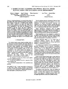
In proposed SA, in order to increase the quality of the solution, some neighborhood generation structures are designed and to increase the searching speed of the proposed SA, some additional termination criteria are presented. The SA algorithm applied in this paper is now described in the fig. 1. For more clarification algorithms, steps are explained bellow:

3) Interchange Techniques (IT) The IT considers exchanges of jobs placed at the ith and jth positions. 4) Insert Neighborhood (IS) The IS inserts the job from the ith position at the jth position. 5) Move Acceptance In order to escape from local minima, the probabilistic acceptance of a non-improving neighbor is used. The probability of accepting a non-improving neighbor is proportional to the temperature T and inversely proportional to the change of the objective function ∆E. So that, the probability of replacing one solution with its neighbor, when ΔE > 0 , is e

−ΔE / Tk

.

Fig. 1. SA proposed algorithm

In this proposed algorithm, SA is used as a local search in ACO algorithm. The Pseudo code of our hybrid algorithm is shown in the fig. 2.

In order to contrast with experimental results in literatures, we conducted a computational experiment by using benchmark problem consist of 29 sets which provided by Carlier and reeves [20-21], and use average relative percentage deviation (ARPD) to measure the solution quality of all algorithms as the following:

Set parameters, initialize pheromone * Cmax =∞

for t=1 to [iteration number] do * Cmax =∞ t

APRD =

for k=1 to [ant-no.] do Repeat

i =1

M ref

*100)

R

As the optimal solution is unknown for the larger instances, the performance of the proposed algorithm is evaluated with a distance from the Rajendran heuristic algorithm [3] and for small instances is evaluated with optimal solutions. The proposed algorithm is compared with 9 other heuristics which can be seen in Table 1-4. DS, DS + M, TS, TS + M and TS + MP are five local search algorithms based on several variants of descending search and tabu search algorithms employed by Garbowski and Pempera [5], the VNS and GA-SA of Schuster and Framinan [6], HPSO represents the results of Liu et al. [22] and HGA of Tseng and Lin [23].

Until ant k make feasible solution k max

: the Object value of generated

k * * k If Cmax then Cmax < Cmax := Cmax t t t t

Apply Local pheromone update end {for} Apply Simulated Annealing Apply Global pheromone update

The results corresponding to the local search based algorithms and the CPU times of them are given in Table I and III, and the results of the population-based algorithms and the CPU times of mentioned algorithms are shown in Table II and IV.

end {for} * Find the best solution value ( Cmax ).

Fig. 2. Pseudo code

IV. COMPUTATIONAL EXPERIMENTS The ACO and ACO-SA algorithm were implemented in Delphi 7.0. Tests were run 15 times for each instances on a dual core 3.6 GH, CPU with 2 GB memory. In the proposed algorithms the parameters were set as follows:

number of ants = 10 ρ = 0.8

q0 =

( M i − M ref )

Where Mi and Mref, were the makespan generated by ACO algorithms and the reference makespan generated by RAJ.

Select item j from N kj with probability Pjk Calculate C feasible loop

R

∑(

( n − 4) ρ n

Table I and II summarizes the computational results reported in [5-6, 22-23] and proposed ACO and ACO-SA algorithms for the small size of instances where optimal solutions are obtained by the branch and bound algorithm. As shown in Table II, the proposed algorithms reach the optimal solution for all of them. In Table III and IV, the computational results reported in [5-6, 22-23] and proposed algorithms are summarized. As illustrated in these Tables, our hybrid algorithm (ACO-SA) is better than all other local search-based algorithms. Most importantly, our algorithm without local search (ACO) is better than three local search-based (GASA, DS, DS+M). Also, analysis of Table IV shows that the performance of ACO-SA algorithm remains competitive. Also, the comparison between ACO and ACO-SA indeed indicate that the SA had very important impact in proposed algorithm, especially in medium and large sizes.

Z =4 Iteration number = 50 T = 40 T f = 0.1 r = 0.85

temp f = 6

counterf = 22

TABLE I. Instance Car01 Car02 Car03 Car04 Car05 Car06 Car07 Car08

M*J 5*11 4*13 5*12 4*14 4*10 9*8 7*7 8*8

optimal 8142 8242 8866 9195 9159 9690 7705 9372

COMPARISON OF LOCAL SEARCH-BASED ALGORITHMS WITH OPTIMAL SOLUTIONS (OPT) VNS

GASA

DS

DS+M

TS

TS+M

TS+MP

PRD

t

PRD

t

PRD

t

PRD

t

PRD

t

PRD

t

PRD

t

0.70 0.20 0.00 1.60 3.50 0.00 0.00 0.00

0 0 0 0 0 0 0 0

0.00 0.00 0.00 0.00 0.00 0.00 0.00 0.00

1 1 1 2 1 1 0 1

0.00 0.62 0.8 2.77 0.00 0.00 0.00 0.00

0.0 0.0 0.0 0.0 0.0 0.0 0.0 0.0

0.00 0.62 0.8 2.77 0.00 0.00 0.00 0.00

0.0 0.0 0.0 0.0 0.0 0.0 0.0 0.0

0.00 0.00 0.00 0.00 0.00 0.00 0.00 0.00

0.1 0.1 0.1 0.1 0.1 0.1 0.1 0.1

0.00 0.00 0.00 0.00 0.00 0.00 0.00 0.00

0.1 0.1 0.1 0.1 0.1 0.1 0.1 0.1

0.00 0.00 0.00 0.00 0.00 0.00 0.00 0.00

0.1 0.1 0.1 0.1 0.1 0.1 0.1 0.1

COMPARISON OF POPULATION-BASED ALGORITHMS WITH OPTIMAL SOLUTIONS (OPT)

TABLE II. Instance

M*J

Name

Car01 Car02 Car03 Car04 Car05 Car06 Car07 Car08

5*11 4*13 5*12 4*14 4*10 9*8 7*7 8*8

HPSO

HGA

ACO

PRD avg

t

PRD avg

t

PRD Min

Avg

t

PRD Min

Avg

t

0.0 0.0 0.0 0.0 0.0 0.0 0.0 0.0

0.4 0.7 0.9 1.4 0.6 0.3 0.2 0.3

0.0 0.0 0.0 0.0 0.0 0.0 0.0 0.0

0.002 0.002 0.002 0.000 0.002 0.000 0.000 0.000

0.00 0.00 0.00 0.00 0.00 0.00 0.00 0.00

0.28 0.27 0.13 0.86 0.00 0.00 0.00 0.00

0.00 0.00 0.00 0.00 0.00 0.00 0.00 0.00

0.00 0.00 0.00 0.00 0.00 0.00 0.00 0.00

0.00 0.00 0.00 0.00 0.00 0.00 0.00 0.00

0.00 0.00 0.00 0.00 0.00 0.00 0.00 0.00

TABLE III. Instance

M*J

RAJ

Name

REC01 REC03 REC05 REC07 REC09 REC11 REC13 REC15 REC17 REC19 REC21 REC23 REC25 REC27 REC29 REC31 REC33 REC35 REC37 REC39 REC41

5*20 5*20 5*20 10*20 10*20 10*20 15*20 15*20 15*20 10*30 10*30 10*30 15*30 15*30 15*30 10*50 10*50 10*50 20*75 20*75 20*75

1590 1457 1637 2119 2141 1946 2709 2691 2740 3157 3015 3030 3835 3655 3583 4631 4770 4718 8979 9158 9344

COMPARISON OF LOCAL SEARCH-BASED ALGORITHMS WITH RAJ

VNS PRD

-2.77 -4.32 -7.03 -2.31 -2.38 -1.54 -5.76 -5.91 -5.15 -7.57 -4.21 -10.76 -5.45 -5.83 -7.23 -4.71 -5.35 -5.51 -10.00 -5.32 -7.41

GASA t

PRD

0 0 0 0 0 0 0 0 0 1 1 0 1 1 1 5 7 7 122 106 110

M*J

RAJ

Name

REC01 REC03 REC05 REC07 REC09 REC11 REC13 REC15 REC17 REC19 REC21 REC23 REC25 REC27 REC29 REC31 REC33 REC35 REC37 REC39 REC41

5*20 5*20 5*20 10*20 10*20 10*20 15*20 15*20 15*20 10*30 10*30 10*30 15*30 15*30 15*30 10*50 10*50 10*50 20*75 20*75 20*75

1590 1457 1637 2119 2141 1946 2709 2691 2740 3157 3015 3030 3835 3655 3583 4631 4770 4718 8979 9158 9344

DS t

-3.96 -4.46 -6.9 -3.45 -4.48 -3.34 -5.65 -6.02 -5.47 -5.45 -2.22 -6.7 -2.69 -2.6 -3.99 2.72 4.78 3.67 5.89 8.80 6.79

TABLE IV. Instance

ACO-SA

6 6 7 12 11 10 17 17 16 34 35 35 55 51 54 147 145 146 907 890 904

DS+M

TS

TS+M

TS+MP

PRD

t

PRD

t

PRD

t

PRD

t

PRD

t

-3.71 -3.43 -5.62 -1.09 -3.6 -1.44 -3.43 -4.83 -5.15 -7.7 -3.68 -7.29 -3.08 -3.64 -7.23 -3.76 -1.97 -4.94 -7.80 -4.97 -6.08

0.00 0.00 0.00 0.00 0.00 0.00 0.00 0.00 0.00 0.00 0.00 0.00 0.00 0.00 0.00 0.10 0.10 0.10 0.10 0.10 0.00

-3.58 -4.43 -5.62 -1.09 -3.6 -1.44 -3.43 -4.83 -5.15 -7.44 -3.68 -7.29 -3.08 -3.64 -7.23 -3.76 -1.97 -4.94 -7.80 -4.97 -6.08

0.00 0.00 0.00 0.00 0.00 0.00 0.00 0.00 0.00 0.00 0.00 0.00 0.00 0.00 0.00 0.00 0.00 0.00 0.00 0.00 0.00

-4.03 -6.59 -7.39 -3.63 -4.62 -3.34 -6.05 -5.91 -5.58 -9.72 -6.31 -10.76 -5.97 -5.64 -7.64 -5.9 -5.51 -6.08 -9.41 -7.00 -8.78

0.2 0.2 0.2 0.2 0.2 0.2 0.3 0.3 0.3 0.4 0.4 0.4 0.5 0.5 0.5 1.1 1.1 1.1 2.5 2.5 2.5

-3.96 -6.59 -7.64 -3.63 -4.58 -3.34 -6.05 -6.02 -5.58 -9.25 -6.3 -10.73 -6.31 -6.1 -8.28 -6.13 -6.31 -6.17 -9.49 -6.99 -8.57

0.2 0.2 0.2 0.2 0.2 0.2 0.3 0.3 0.3 0.4 0.4 0.4 0.5 0.5 0.5 1.1 1.1 1.1 2.6 2.6 2.6

-3.96 -6.59 -7.7 -3.63 -4.58 -3.34 -6.05 -5.91 -5.58 -9.38 -6.17 -10.89 -6.21 -5.83 -7.94 -6.22 -6.37 -5.91 -9.36 -6.91 -8.82

0.2 0.2 0.2 0.2 0.2 0.2 0.3 0.3 0.3 0.4 0.4 0.4 0.5 0.5 0.5 1.1 1.1 1.1 2.6 2.6 2.6

COMPARISON OF POPULATION-BASED ALGORITHMS WITH RAJ HPSO

HGA

PRD

PRD

ACO

ACO-SA

PRD

PRD

avg

t

avg

t

Min

Avg

-3.77 -6.59 -7.39 -3.63 -4.58 -3.34 -6.05 -6.02 -5.58 -9.15 -5.70 -10.8 -5.71 -6.13 -7.81 -5.92 -5.51 -6.02 -8.89 -6.79 -7.94

3.9 4.8 4.1 6.6 6.7 7.0 11.0 8.6 8.6 23.0 24.0 24.0 32.0 39.0 31.0 122.0 116.0 105.0 635.0 897.0 883.0

-4.03 -6.59 -7.70 -3.63 -4.62 -3.34 -6.05 -6.02 -5.58 -9.72 -6.17 -10.89 -6.31 -6.13 -8.15 -6.41 -6.54 -6.23 -9.56 -7.13 -8.98

0.009 0.006 0.008 0.008 0.008 0.008 0.009 0.008 0.008 0.034 0.03 0.025 0.031 0.031 0.031 0.267 0.252 0.225 1.447 1.283 1.073

-3.52 -5.4 -6.96 -3.44 -3.6 -2.98 -5.8 -5.9 -5.47 -8.11 -5.30 -8.81 -5.45 -4.57 -6.67 -4.71 -4.57 -4.3 -7.60 -5.49 -6.30

-3.28 -5.1 -6.33 -3.09 -3.10 -2.46 -5.5 -5.64 -5.27 -7.57 -4.7 -8.58 -4.95 -3.58 -6.21 -4.27 -3.48 -3.7 -7.19 -4.95 -5.81

t

0.01 0.00 0.01 0.00 0.00 0.01 0.01 0.00 0.00 0.05 0.04 0.04 0.03 0.05 0.06 0.011 0.011 0.012 0.026 0.026 0.026

Min

Avg

-4.03 -6.59 -7.68 -3.63 -4.62 -3.34 -6.05 -6.02 -5.58 -9.72 -6.43 -10.89 -6.31 -6.12 -8.15 -6.41 -6.83 -6.42 -9.88 -7.31 -8.92

-4.03 -6.52 -7.64 -3.63 -4.6 -3.34 -6.05 -6.02 -5.55 -9.67 -6.33 -10.78 -6.23 -6.04 -8.08 -6.29 -6.59 -6.29 -9.68 -7.23 -8.79

t

0.029 0.022 0.019 0.022 0.025 0.023 0.026 0.036 0.022 0.048 0.059 0.050 0.093 0.115 0.096 0.39 0.48 0.46 1.581 1.595 1.409

V. CONCLUSIONS In the current research, a no-wait flowshop scheduling problem for minimizing the makespan was discussed. This problem is known to be strongly NP-hard. In this paper, ACO with a local search based on simulated annealing is proposed to solve this problem. Comparison of the proposed algorithm with 9 other heuristics demonstrates the efficiency of the ACO-SA algorithm. Computational results show that the proposed algorithm can reach an optimal solution for the small size problems while in larger size problems; the algorithm is still competitive to the best reported algorithms. REFERENCES [1]

[2] [3] [4] [5]

[6]

[7]

[8]

[9]

[10]

[11] [12] [13]

[14] [15]

[16]

[17]

[18]

N. G. Hall and Sriskandarajah, “A survey of machine scheduling problems with locking and no-wait in process,” Operations Research, vol. 44, pp. 510-525, 1996. M. R. Garay and D. S. Johnson, Computers and Intractability: A Guide to the Theory of NP-Completeness. SanFrancisco: Freedman, 1979. C. Rajendran, “A no-wait flowshop scheduling heuristic to minimize makespan,”Operational Research Societ, vol. 45, pp. 472-478, 1994. A. Fink, S. Voβ, “Solving the continuous flowshop scheduling problem by metaheuristics,” Eur J Oper Res, vol. 151,pp. 400-414, 2003. J. Grabowski and J. Pempera, “Some local search algorithms for no-wait flowshop problem with makespan criterion,” Computers & Operations Research, vol. 32, pp. 2197-2212, 2005. C. J. Schuster and J. M. Framinan, “Approximative procedures for nowait job shop scheduling,” Operations Research Letters, vol. 31, pp. 308-318, 2003. C. L. Chen, R. V. Neppali, and N. Aljaber, “Genetic algorithms applied to the continuous flowshop problem,” Computers & Industrial Engineering, vol. 30, pp. 919-929, 1996. S. J. Shyu, B. M. T. Lin, and P. Y. Yin, “Application of ant colony optimization for no-wait flowshop scheduling problem to minimize the total completion time,” Computers & Industrial Engineering, vol. 47, pp. 181-193, 2004. Q-K. Pan, M. F. Tasgetiren, and Y-C. Liang, “A discrete particle swarm optimization algorithm for the no-wait flowshop scheduling problem,” Computers & Operations Research, vol. 35, pp. 2807-2839, 2008. A. Colorni, M. Dorigo, and Maniezzo, “Distributed optimization by ant colonies,” Proceedings of the First European Conference on Artificial Life, Paris, 1991. M. Dorido and G. DiCaro, and L. M. Gambardella, “Ant algorithms for discrete optimization,” Artificial Life, vol. 5, pp. 137-172, 1999. T. Stutzle, “An ant approach to the flowshop problem,” Proceedings of EUFIT’98, Aachen, pp. 1560-1564, 1998. T. Stutzle and H. Hoos, “The max-min ant system and local search for the traveling salesman problem,” Proceedings of ICEC, vol. 97, pp. 309314, 1997. R. W. Eglese, “simulated annealing: a tool for operational research,” European Journal of Operational Research, vol. 46, pp. 271-281, 1990. P. J. M. Van Laarhoven, E. H. L. Aarts and J. K. Lenstra, “Job shop scheduling by simulated annealing,” Operation Research, vol. 40, pp. 113-125, 1992. S. H. Zegoridi, K. Itoh and T. Enkawa,”Minimization makespan for flowshop scheduling by combining simulated annealing with sequencing knowledge” European Journal of Operational Research, vol. 85, pp. 515-531, 1995. L. Dipak and U. K. Chakraborty,”An efficient hybrid heuristic for makespan minimization in permutation flowshop scheduling” The International Journal of Advanced Manufacturing Technology, vol. 44. pp. 559-569, 2009. C. Rajendran and H. Ziegler, “Ant colony algorithm for permutation flowshop scheduling to minimize makespan/total flowtime of jobs,” European Journal of Operational Research, vol. 155, pp. 426-438, 2004.

[19] D. Merkle and M. Middendorf, “An ant algorithm with a new pheromone evaluation rule for total tardiness problems,” Applied Intelligence, vol. 18, pp. 105-111, 2003. [20] J. Carlier, “Ordonnancements a contraints disjonctives,” RAIRO Recherche operationelle, vol. 12, pp. 331-351, 1978. [21] C. Reeves, “A genetic algorithm for flowshop sequencing,” Computers and Operations Research, vol. 22, pp. 5-13, 1995. [22] B. Liu, L. Wang and Y. H. Jin, “An effective hybrid particle swarm optimization for no-wait flowshop scheduling,” International Journal of Advanced Manufacturing Technology, vol. 31, pp. 1001–1011, 2007. [23] L-Y. Tseng and Y-T. Lin, “A hybrid genetic algorithm for no-wait flowshop scheduling problem,” International Journal of Production Economics, vol. 128, pp. 144-152, 2010.