A hybrid method for computing the smallest eigenvalue of a symmetric

A hybrid method for computing the smallest eigenvalue of a symmetric and positive definite Toeplitz matrix Heinrich Voss∗

Aleksandra Kosti´c

January 15, 2003

Abstract In this paper we suggest a hybrid method for computing the smallest eigenvalue of a symmetric and positive definite Toeplitz matrix which takes advantage of two types of methods, Newton’s method for the characteristic polynomial and projection methods based on rational interpolation of the secular equation.

Keywords: Toeplitz matrix, eigenvalue problem, hybrid method AMS Subject Classification:

1

65F15

Introduction

The problem of finding the smallest eigenvalue λ1 of a real symmetric, positive definite Toeplitz matrix T is of considerable interest in signal processing. Given the covariance sequence of the observed data, Pisarenko [13] suggested a method which determines the sinusoidal frequencies from the eigenvector of the covariance matrix associated with its minimum eigenvalue. Several methods have been reported in the literature for computing the minimum eigenvalue of T , cf. [2], [4], [5], [6], [7], [8], [9], [10], [11], [12], [15], [16], [17], e.g. In their seminal paper Cybenko and Van Loan [2] presented the following method: by bisection they determine an initial approximation µ0 ∈ (λ1 , ω1 ), ∗ Hamburg University of Technology, Department of Mathematics, D-21071 Hamburg, Federal Republic of Germany, ({kostic,voss}@tu-harburg.de)

1

A HYBRID METHOD FOR THE TOEPLITZ EIGENPOBLEM

2

where ω1 denotes the smallest pole of the secular equation f , and they improve µ0 by Newton’s method for f which converges monotonely and quadratically to λ1 . This approach was improved considerably by Mackens and the second author by replacing Newton’s method by a more appropriate root finding method for the secular equation, which is a rational function where the wanted root λ1 and the smallest pole ω1 can be very close to each other. Namely, we used a root finding method based on rational Hermitean interpolation in [8], and since this one turned out to be equivalent to a projection method where the eigenvalue problem for T is projected to a two dimensional subspace it could be improved further in [9]. The root finding phase of the approach usually converges very fast whereas the bisection phase can be very costly since no procedure is known how to obtain an initial value µ0 ∈ (λ1 , ω1 ) efficiently. Mastronardi and Boley [11] suggested Newton’s method for the characteristic polynomial χn of T which can be enhanced by a double step strategy and/or by Hermitean interpolation of the characteristic polynomial (cf. [10]). The advantage of this method upon Cybenko and Van Loan’s approach is its conceptual simplicity, and its monotone convergence from below starting with any lower bound of λ1 , for instance with the initial guess µ0 = 0. However, this convergence usually is slower than that of the root finding method mentioned in the last paragraph. To conclude, for the secular equation Newton’s method requires an expensive preprocessing to obtain a suitable initial value which is not the case for the characteristic polynomial. On the other hand every single step is less expensive for the secular equation, and the convergence usually is faster. It is interesting to note that the dominant share of the cost for each step of both types of methods is the solution of a Yule–Walker system to evaluate the secular equation and its derivative at a guess λ and the characteristic polynomial of T , respectively. This property suggests to combine both methods in a hybrid approach, and to gather information about one method while performing an iteration step of the other one, thus squeezing the most out of a Yule–Walker solve. In this paper we propose a method of this type. We start with Newton’s method for the characteristic polynomial getting lower bounds of the smallest eigenvalue λ1 . Concurrently we obtain upper bounds of λ1 from rational interpolations of the secular equation which then yield a good approximation to λ1 as initial guess for the projection method mentioned above. While evaluating the secular function f in projection steps, at the same time we obtain for free lower bounds of the smallest root ω1 of the characteristic polynomial of the principal submatrix of T of dimension n − 1. A further

A HYBRID METHOD FOR THE TOEPLITZ EIGENPOBLEM

3

rational interpolation of f then yields good lower bounds of λ1 thus gaining an efficient stopping criterion. The paper is organized as follows. Section 2 summarizes properties of the underlying methods using the characteristic polynomial and the secular equation, respectively. Section 3 suggests the new hybrid method including the improved stopping criterion, and Section 4 demonstrates its efficiency by numerical examples. The paper closes with concluding remarks concerning the use of superfast Toeplitz solvers.

2

Basic approaches

Let Tn = (t|i−j| ) ∈ Rn×n be a symmetric and positive definite Toeplitz matrix. We consider the problem to determine the smallest eigenvalue (and corresponding eigenvector) of Tn . In this section we summarize two basic methods which will be used in the next section to form a hybrid method. Mastronardi and Boley suggested to determine the smallest eigenvalue λ1 of Tn by Newton’s method for the characteristic polynomial of Tn . Denote the j-dimensional principal submatrix of Tn by Tj , and the first column of Tj+1 omitting the diagonal entry t0 by t(j) := (t1 , t2 , . . . , tj−1 , tj )T . If λ is not an eigenvalue of Tj then µ ¶µ ¶ 1 0T t0 − λ + (t(j) )T y (j) (λ) −(y (j) (λ))T Tj+1 −λIj+1 = 0 Ij t(j) Tj − λIj where y (j) (λ) denotes the solution of the j-th Yule-Walker system (Tj − λIj )y (j) (λ) = −t(j) . Hence, if λ is not in the spectrum of any of the principal submatrices Tj , j = 1, . . . , n − 1, then the characteristic polynomials χj (λ) := det(Tj − λIj ) of Tj satisfy the recurrence relation χj+1 (λ) = χj (λ)(t0 − λ + (t(j) )T y (j) (λ)) =: χj (λ)βj (λ),

1 ≤ j ≤ n − 1,

and for the derivatives it holds that χ′j+1 (λ) = χ′j (λ)βj (λ) − χj (λ)(1 + ky (j) (λ)k22 ). Durbin’s algorithm (cf.[3], p. 194 ff) for the Yule–Walker system (Tn−1 − λIn−1 )y (n−1) (λ) = −t(n−1)

A HYBRID METHOD FOR THE TOEPLITZ EIGENPOBLEM

4

yields the parameters βj (λ) and the vectors y (j) (λ), j = 1, . . . , n − 1. Hence, the characteristic polynomial χn (λ) can be evaluated using Durbin’s algorithm, and the cost of one evaluation is 2n2 +O(n) flops. With n2 additional flops to determine ky (j) (λ)k22 , j = 1, . . . , n−1 one can evaluate the derivative χ′n (λ) as well. Therefore, one Newton step for the characteristic polynomial requires 3n2 + O(n) flops. For λ < λ1 the characteristic polynomial χn (λ) is convex and monotonically decreasing, and thus for every initial value µ0 < λ1 (for instance µ0 = 0) Newton’s method converges from the left to the smallest eigenvalue of Tn . For the same reason the secant method converges monotonically increasing to λ1 if the initial guesses µ0 , µ1 satisfy µ0 < µ1 ≤ λ1 . Newton’s method and the secant method very often converge slowly in the beginning if the initial value µ0 is far from the smallest root of χn or if the slope of χn is very large. In our numerical examples we observed up to 45 Newton steps to determine the smallest eigenvalue up to a relative error 10−6 , and the secant method converges even slowlier. The global behaviour of both methods can be improved considerably by a double step strategy. Theorem 1 (Stoer and Bulirsch [14], p. 274) Let χ(λ) be a polynomial of degree n > 2, all roots of which are real, λ1 ≤ λ2 ≤ · · · ≤ λn . Let ξ1 be the smallest root of χ′ (λ). Then for every µ < λ1 the numbers µ′ := µ −

χ(µ) χ(µ) χ(ν) , ν := µ − 2 ′ , ν ′ := ν − ′ ′ χ (µ) χ (µ) χ (ν)

are well defined, and they satisfy ν < ξ1 , and µ′ ≤ ν ′ ≤ λ1 . Theorem 1 suggests the following acceleration of Newton’s method: Double steps χn (µk ) µk+1 := µk − 2 ′ χn (µk ) are performed until µk+1 > λ1 , which is signaled by the change of sign of the Newton increment. Then the method switches to the original Newton method. An analogous result holds for the secant method. One drawback of Newton’s method and the secant method is that they take advantage only of the last iterate and the last two iterates, respectively, but they do not use information gained in previous steps. Improvements employing interpolations of previous iterates were proposed in [10]. However, we do not take advantage of these modifications in the hybrid method considered here. A different approach for computing the smallest eigenvalue λ1 of Tn was suggested by Cybenko and Van Loan [2] who determined λ1 as the smallest

A HYBRID METHOD FOR THE TOEPLITZ EIGENPOBLEM

5

root of the secular function f (λ) =

−χn (λ) = −t0 + λ + (t(n−1) )T y (n−1) (λ) = −βn−1 (λ) χn−1 (λ)

which can be evaluated by Durbin’s algorithm as well. Since f ′ (λ) = 1 + ky (n−1) (λ)k2 , the evaluation of f ′ (λ) then essentially comes for free, and for the secular equation a Newton step requires only 2n2 + O(n) flops. Let ω1 denote the smallest eigenvalue of Tn−1 , i.e. the smallest pole of f . Then f is monotonically increasing and convex for λ < ω1 , and therefore Newton’s method for the secular equation converges monotonically decreasing for every initial value µ0 ∈ [λ1 , ω1 ). Cybenko and Van Loan [2] suggested to determine a suitable initial value µ0 by bisection based on Durbin’s algorithm. If µ is not in the spectrum of any of the principal submatrices of Tn −µIn then Durbin’s algorithm applied to Tn − µIn determines a unit left triangular matrix L and a diagonal matrix D such that L(Tn − µIn )LT = D := diag{1, δ1 , . . . , δn−1 }. Hence, from Sylvester’s law of inertia one gets µ < λ1 , if δj > 0 for j = 1, . . . , n − 1, µ ∈ [λ1 , ω1 ), if δj > 0 for j = 1, . . . , n − 2 and δn−1 ≤ 0, and µ > ω1 , if δj < 0 for some j ∈ {1, . . . , n − 2}. Hence, for the secular equation Newton’s method requires an expensive preprocessing to obtain a suitable initial value which is not the case for the characteristic polynomial. On the other hand every single step is less expensive for the secular equation, and the convergence usually is faster. Since both methods use Durbin’s algorithm as a basic building block it is reasonable to combine both methods in a hybrid approach. Actually, we combine the Newton process for the characteristic polynomial with a modification of Cybenko’s and Van Loan’s method. The global convergence behaviour of Newton’s method for the secular equation usually is not satisfactory since the smallest root λ1 and the smallest pole ω1 of the rational function f can be very close to each other. In this situation the initial steps of Newton’s method are extremely slow, at least if the initial guess is close to ω1 . Approximating the secular equation by a suitable rational function the convergence of the method can be improved considerably. f can be rewritten

A HYBRID METHOD FOR THE TOEPLITZ EIGENPOBLEM

6

as (1)

f (λ) = f (0) + λf ′ (0) + λ2

n−1 X j=1

αj2 ωj − λ

where αj are real numbers depending on the eigenvectors of Tn−1 and ωj denote the eigenvalues of Tn−1 ordered by magnitude (cf. [8]), and with a shift µ which is not in the spectrum of Tn−1 it obtains the form (2)

f (λ) = f (µ) + (λ − µ)f ′ (µ) + (λ − µ)2 φ(λ; µ)

where (3)

φ(λ; µ) =

n−1 X j=1

αj2 γj2 , ωj − λ

γj =

ωj . ωj − µ

The representation (1) of f suggests to replace the linearization of f in Newton’s method by a root finding method based on a rational model (4)

g(λ; µ) = f (0) + λf ′ (0) + λ2

b , c−λ

where µ is a given approximation to λ1 and b and c are determined such that (5)

g(µ; µ) = f (µ), g ′ (µ; µ) = f ′ (µ).

For this modification the following convergence result was proved in [8]. Theorem 2: Let g be given by (4) and (5) where µ is not in the spectrum of Tn−1 , and denote by ρ(µ) the smallest positive root of g(·; µ). Then ρ(µ) ≥ λ1 . If µ0 ∈ (λ1 , ω1 ) and µk+1 = ρ(µk ), then the sequence {µk } converges monotonically decreasing to λ1 , the convergence is quadratic, and it is faster than Newton’s method, i.e. if νk+1 = µk − f (µk )/f ′ (µk ) then λ1 ≤ µk+1 ≤ νk+1 . In [9] it was shown that ρ(µ) is the smallest eigenvalue of the projected eigenproblem [q(0), q(µ)]T Tn [q(0), q(µ)]y = κ[q(0), q(µ)]T [q(0), q(µ)]y where q(µ) solves the linear system (Tn − µI)q(µ) = −f (µ)e1 ,

A HYBRID METHOD FOR THE TOEPLITZ EIGENPOBLEM

7

and e1 is the unit vector containing a 1 in its first component and 0 anywhere else. This result suggests to improve the method further by defining µk+1 as the smallest eigenvalue of the projected problem Ak y := QTk Tn Qk y = κQTk Qk y =: κBk y,

for Qk = [q(0), q(µ1 ), . . . , q(µk )]

where µ1 , . . . , µk ∈ (0, ω1 ) are parameters obtained in the course of the algorithm. It is interesting to note that every step essentially requires one YuleWalker solve since ½ ′ f (µ) for µ = ν q(µ)T q(ν) = (f (µ) − f (ν))/(µ − ν) for µ 6= ν and q(µ)T Tn q(ν) = −f (µ) + µq(µ)T q(ν). For this method the following convergence result was proved in [9] by comparison with inverse iteration with Rayleigh quotient shifts. Theorem 3 Let µ1 , . . . , µℓ−1 be not in the spectrum of Tn−1 , let µℓ ∈ (λ1 , ω1 ), and for k ≥ ℓ let µk+1 be the smallest eigenvalue of the projected problem Ak y = κBk y. Then the sequence {µk } converges monotonically decreasing to λ1 , and the convergence is at least cubic.

3

A HYBRID METHOD

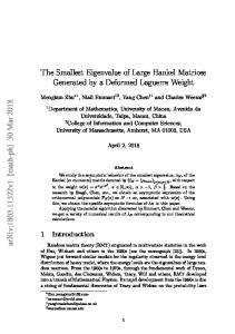
We are now in the position to draft a hybrid algorithm. We start with a Newton step for the characteristic polynomial χn with initial guess µ0 = 0 followed by a secant step yielding the lower bounds µ0 < µ1 < µ2 < λ1 . We evaluate f at µ0 , µ1 and µ2 , where f (µ0 ) and f (µ1 ) come for free, and determine the smallest positive roots ρj of g(·; µj ) for j = 1, 2, and the projected matrices A2 and B2 . Since λ1 is the smallest fixed point of ρ(·) the fixed point µ3 of the linear interpolation of (µ1 , ρ1 ) and (µ2 , ρ2 ) should be a reasonable approximation to λ1 . Figure 1 contains the graph of ρ and the linear interpolation with fixed points λ1 and µ3 , respectively, for 2 examples, a typical one on the left and a less typical one on the right. Although in the example on the right the linear interpolation is far from being a good approximation to ρ its fixed point µ3 is a reasonable approximation to ρ’s fixed point λ1 .

A HYBRID METHOD FOR THE TOEPLITZ EIGENPOBLEM

−3

x 10

8.5 µ1

8

µ2

µ3

7.5

7

6.5

λ1

6 0

1

2

3

4

5

6

7

8 −3

x 10 −5

10

x 10

9.8 9.6

µ1

9.4

µ2 µ

9.2

3

9 8.8 8.6 8.4

λ

1

8.2 0

0.2

0.4

0.6

0.8

1 −4

x 10

Figure 1: Fixed point of ρ(·) and of linear interpolation of ρ(·)

8

A HYBRID METHOD FOR THE TOEPLITZ EIGENPOBLEM

9

Table 1: Accuracy of interpolation / Distance of root and pole dim. 32 64 128 256 512 1024 2048

relative error of µ3 max 9.69E − 02 1.20E − 01 2.87E − 01 1.59E − 01 2.31E − 01 1.93E − 01 2.75E − 01

average 1.01E − 02 1.49E − 02 2.03E − 02 1.89E − 02 2.35E − 02 2.62E − 02 2.61E − 02

rel. distance of λ1 and ω1 min 6.07E − 03 7.31E − 04 5.86E − 04 4.25E − 04 2.70E − 05 1.33E − 05 1.32E − 05

average 3.94E − 01 2.22E − 01 1.32E − 01 7.22E − 02 3.96E − 02 1.94E − 02 1.21E − 02

To test the accuracy of the approximation µ3 to λ1 we considered Toeplitz matrices n X ηk T2πθk , Tθ = (tij ) = (cos(θ(i − j))) T = k=1

where ηk and θk are uniformly distributed random numbers taken from [0, 1] (cf. Cybenko and Van Loan [2]). For each of the dimensions n = 32, 64, 128, 256, 512, 1024 and n = 2048 we considered 100 test problems. On the left hand Table I contains the maximum relative error and the average of relative errors of µ3 . If µ3 is less than ω1 then we update the matrices A2 and B2 and continue with the projection method outlined in Section 2. For µ3 ∈ (λ1 , ω1 ) we then obtain monotone convergence to λ1 . It may happen that µ3 > ω1 or that the smallest eigenvalue µj of Aj−1 y = µBj−1 y for some j ≥ 4 is greater than ω1 . Since Durbin’s algorithm is known to be stable only for a positive definite system matrix (cf. [1]), i.e. since the evaluation of f (µ) is known to be stable only for µ < ω1 , we do not take into consideration parameters µj > ω1 in the projection method. In this case we replace µj by the weighted bisection µj ← 0.1˜ µ + 0.9µj where µ ˜ := max{µk < λ1 : 2 ≤ k ≤ j − 1}. The smallest root λ1 and the smallest pole ω1 may be very close to each other (Table I on the right contains the minimum relative distance and the average of relative distances in our test examples), and it may happen that the method bounces between lower bounds of λ1 obtained from the weighted bisection and upper bounds of ω1 obtained as smallest eigenvalues of projected problems. We remedy this behaviour by the following tie break rule which was introduced in [8] for the method based on root finding by

A HYBRID METHOD FOR THE TOEPLITZ EIGENPOBLEM

10

rational Hermitean interpolation. If µj < λ1 then we evaluate f (µj ) and f ′ (µj ) to update Aj−1 and Bj−1 , and we determine µj+1 as smallest eigenvalue of Aj y = µBj y. It is obvious that we get for free a further upper bound µ ˜j+1 = µj − f (µj )/f ′ (µj ) from Newton’s method, where both approximations, µ ˜j+1 and µj+1 correspond to quadratically or even cubically convergent processes. If the relative distance of these two bounds is not small then µj cannot be a good approximation to λ1 , and it is not unlikely that µj+1 > ω1 . Hence, if |µj+1 − µ ˜j+1 |/µj+1 > 0.01 then we replace µj+1 by µj+1 ← 0.1µj + 0.9µj+1 . Until now we applied the characteristic polynomial of Tn only to construct an initial guess for the projection method. While evaluating f (µk ) in subsequent steps of the projection method we make further use of the characteristic polynomial χn−1 (µk ) of the principal submatrix Tn−1 (which comes for free) to terminate the method efficiently. The termination is based on the following Theorem which yields a lower bound of λ1 using a further rational interpolation of the secular equation. In distinction to the rational approximation of f in (4) and (5) here the pole is a fixed lower bound of ω1 . Theorem 4: Let κ ∈ (0, λ1 ), µ ∈ (κ, ω1 ) and p ∈ (κ, ω1 ). Let h(λ) := f (µ) + f ′ (µ)(λ − µ) + (λ − µ)2

b , p−λ

where b is determined such that the interpolation condition h(κ) = f (κ) holds. Then b > 0, i.e. h is strictly monotonically increasing and strictly convex in (0, p), and the unique root of h in (0, p) is a lower bound of λ1 . Proof: From equation (2) and from the interpolation condition h(κ) = f (κ) we obtain b = (p − κ)φ(κ; µ) > 0. ˜ of h in (0, p) is a lower bound of λ1 is obvious for That the unique root λ p ≤ λ1 . For p > λ1 we have to show h(λ1 ) > 0. This follows from equations (2) and (3):

A HYBRID METHOD FOR THE TOEPLITZ EIGENPOBLEM

11

b h(λ1 ) = f (µ) + f ′ (µ)(λ1 − µ) + (λ1 − µ)2 p − λ1 ¶ µ (p − κ)φ(κ; µ) 2 = f (λ1 ) − (λ1 − µ) φ(λ1 ; µ) − p − λ1 2 (λ1 − µ) ((p − κ)φ(κ; µ) − (p − λ1 )φ(λ1 ; µ)) = p − λ1 µ ¶ n−1 (λ1 − µ)2 X 2 2 p − κ p − λ1 = − αj γj p − λ1 ωj − κ ωj − λ 1 j=1

=

n−1 µ)2 X

(λ1 − p − λ1

j=1

αj2 γj2

(ωj − p)(λ1 − κ) > 0. ¤ (ωj − κ)(ωj − λ1 )

Since the algorithm eventually enters the interval (λ1 , ω1 ) we obtain a suitable lower bound p of ω1 in the course of the algorithm. We can even do a little better. ω1 is the smallest root of the characteristic polynomial χn−1 of Tn−1 , all roots of which are real. Hence, given two lower bounds µk and µk+1 of ω1 a secant step for χn−1 with these parameters yields a lower bound of ω1 , too, which is bigger than max{µk , µk+1 }. Notice that evaluating f by Durbin’s algorithm at some µ we get χn−1 (µ) for free. Putting these considerations together we end up with Algorithm 1.

4

NUMERICAL EXPERIMENTS

We applied the hybrid method to the test examples mentioned in the last section. Table II contains the average number of flops and the average number of Durbin steps needed to determine the smallest eigenvalue in 100 test problems where the iteration was terminated if the error was guaranteed to be less than 10−6 . For comparison we added the cost of the projection method in [9], and a Newton type method for the characteristic polynomial in [10] which uses previous iterations in a Hermitean interpolation. Notice that every step of the projection method and the hybrid method requires 2n2 + O(n) flops whereas every step of the Newton type method requires 3n2 + O(n) flops. We already mentioned in Section 2 that Newton’s method and the secant iteration for the characteristic polynomial can be accelerated using double steps, and of course these can be introduced in the initial phase of the hybrid method, too. However, then it may happen that after the first double

A HYBRID METHOD FOR THE TOEPLITZ EIGENPOBLEM

Algorithm 1 Hybrid method for computing the smallest eigenvalue 1: Initial guess µ0 = 0 2: Determine µ1 by Newton’s method and µ2 by secant method for χn simultaneously for j = 1, 2 determine roots ρj of g(·; µj ) simultaneously determine matrices A2 and B2 store best known lower bound λℓ = µ2 and minimum eigenvalue of A2 y = µB2 y as upper bound λu of λ1 determine lower bound p of ω1 by secant step for χn−1 3: Determine fixed point µ3 of linear interpolation of (µj , ρj ), j = 1, 2 4: for k = 3, 4, . . . until convergence do 5: Evaluate f (µk ), f ′ (µk ), χn−1 (µk ) by Durbin’s algorithm and decide whether µk < λ1 or µk ∈ (λ1 , ω1 ) or µk > ω1 6: if µk > ω1 then 7: λu = min{λu , µk } 8: µk ← 0.1 ∗ λℓ + 0.9 ∗ λu 9: else 10: update Ak−1 → Ak and Bk−1 → Bk 11: determine smallest eigenvalue ν of Ak y = µBk y 12: λu = min{λu , ν} 13: determine new lower bound p of ω1 by secant step for χn−1 and new lower bound λℓ of λ1 using Theorem 4 14: if µk ∈ (λ1 , ω1 ) then 15: µk+1 = λu 16: else 17: λnewton = µk − f (µk )/f ′ (µk ) 18: if |λnewton − ν|/ν| < 0.01 then 19: µk+1 = ν 20: else 21: µk+1 = 0.1 ∗ λℓ + 0.9 ∗ ν 22: end if 23: end if 24: end if 25: end for

12

A HYBRID METHOD FOR THE TOEPLITZ EIGENPOBLEM

13

Table 2: Average number of flops and Durbin calls dim. 32 64 128 256 512 1024 2048

projection flops 1.226E04 4.716E04 1.871E05 8.242E05 3.582E06 1.523E07 6.588E07

Newton type

steps 4.49 5.08 5.41 6.13 6.75 7.22 7.83

flops 1.759E04 6.171E04 2.113E05 8.861E05 3.968E06 1.627E07 6.593E07

steps 4.01 4.36 4.10 4.42 5.00 5.15 5.23

hybrid flops 1.418E4 5.248E4 2.047E5 8.295E5 3.456E6 1.463E7 5.728E7

steps 4.92 5.27 5.46 5.69 6.02 6.44 6.31

Table 3: Cost of hybrid method and its modification dim. 32 64 128 256 512 1024 2048

hybrid flops 1.418E4 5.248E4 2.047E5 8.295E5 3.456E6 1.463E7 5.728E7

modification steps 4.92 5.27 5.46 5.69 6.02 6.44 6.31

flops 1.308E4 4.992E4 1.880E5 7.666E5 3.180E6 1.339E7 5.459E7

steps 4.48 4.98 4.97 5.22 5.50 5.85 5.99

Newton step µ1 > ω1 or λ1 < µ1 < ω1 . In both cases we continue directly with the projection method where for µ1 > ω1 we first replace µ1 by µ1 ← 0.5µ1 , i.e. the single Newton step. Similarly, if µ1 < λ1 and the iterate µ2 of a double secant step satisfies µ2 > λ1 then we continue directly with the projection method, and again we replace µ2 by the result of a single secant step if µ2 > ω1 . If µ1 < µ2 < λ1 then we determine µ3 by linear interpolation of ρ and proceed as in the hybrid method above. These modifications yield a further improvement of the method. Table III contains the average number of flops and Durbin calls for the hybrid method and its modification.

5

CONCLUDING REMARKS

We have presented a hybrid method for computing the smallest eigenvalue of a symmetric and positive definite Toeplitz matrix taking advantage of

A HYBRID METHOD FOR THE TOEPLITZ EIGENPOBLEM

14

both types of methods, Newton’s method for the characteristic polynomial and projection methods based on rational approximations of the secular equation. At least for high dimensions these methods yield noteworthy improvements over the underlying approaches. We used Durbin’s method to solve the occurring Yule-Walker equations and to determine the Schur parameters δj requiring 2n2 + O(n) flops. Of course this could have been done by superfast Toeplitz solvers the complexity of which is only O(n log2 n) operations. Notice however, that this pays only if the dimension n is larger than 512. In a similar way as in [15] the method can be further enhanced taking advantage of symmetry properties of the eigenvectors of a symmetric Toeplitz matrix.

References [1] Cybenko G. The numerical stability of the Levinson-Durbin algorithm for Toeplitz systems of equations. SIAM J. Sci. Stat. Comput. 1980; 1: 303–309 [2] Cybenko G, Van Loan CF. Computing the minimum eigenvalue of a symmetric positive definite Toeplitz matrix. SIAM J. Sci. Stat. Comput. 1986; 7: 123–131 [3] Golub GH, Van Loan CF. Matrix Computations (3rd edn). The John Hopkins University Press: Baltimore and London 1996 [4] Hu YH, Kung SY. Toeplitz eigensystem solver. IEEE Trans. Acoustics, Speech, Signal Processing 1985; 33: 1264–1271 [5] Huckle T. Computing the minimum eigenvalue of a symmetric positive definite Toeplitz matrix with spectral transformation Lanczos method. In Numerical Treatment of Eigenvalue Problems, Vol. 5 Albrecht J, Collatz L, Hagedorn P, Velte W (eds). Birkh¨auser: Basel 1991; 109–115 [6] Huckle T. Circulant and skewcirculant matrices for solving Toeplitz matrices. SIAM J. Matr. Anal. Appl. 1992; 13: 767–777 √ [7] Kosti´c A, Voss H. A method of order 1 + 3 for computing the smallest eigenvalue of a symmetric Toeplitz matrix. WSEAS Transactions on Mathematics 2002; 1: 1–6 [8] Mackens W, Voss H. The minimum eigenvalue of a symmetric positive definite Toeplitz matrix and rational Hermitian interpolation. SIAM J. Matr. Anal. Appl. 1997; 18: 521–534

A HYBRID METHOD FOR THE TOEPLITZ EIGENPOBLEM

15

[9] Mackens W, Voss H. A projection method for computing the minimum eigenvalue of a symmetric positive definite Toeplitz matrix. Lin. Alg. Appl. 1998; 275–276: 401–415 [10] Mackens W, Voss H. Computing the minimum eigenvalue of a symmetric positive definite Toeplitz matrix by Newton type methods. SIAM J. Sci. Comput. 2000: 21: 1650–1656 [11] Mastronardi N, Boley D. Computing the smallest eigenpair of a symmetric positive definite Toeplitz matrix. SIAM J. Sci. Comput. 1999; 20: 1921–1927 [12] Melman A. Extreme eigenvalues of real symmetric Toeplitz matrices. Math. Comp. 2000; 70: 649–669 [13] Pisarenko VF. The retrieval of harmonics from a covariance function. Geophys. J. R. astr. Soc. 1973; 33: 347–366 [14] Stoer J, Bulirsch R. Introduction to Numerical Analysis. Springer: New York 1980 [15] Voss H. Symmetric schemes for computing the minimum eigenvalue of a symmetric Toeplitz matrix. Lin. Alg. Appl. 1999; 287: 359–371 [16] Voss H. A symmetry exploiting Lanczos method for symmetric Toeplitz matrices. Numerical Algorithms 2000; 25: 377–385 [17] Voss H. A variant of the inverted Lanczos method. BIT Numerical Analysis 2001; 41: 1111–1120