A Hybrid Multi-population Framework for Dynamic Environments ...

Soft Computing Journal manuscript No. (will be inserted by the editor)

A Hybrid Multi-population Framework for Dynamic Environments Combining Online and Offline Learning ¨ G¨ on¨ ul Uluda˘ g · Berna Kiraz · A. S ¸ ima Etaner-Uyar · Ender Ozcan

Received: date / Accepted: date

Abstract Population based incremental learning algorithms and selection hyper-heuristics are highly adaptive methods which can handle different types of dynamism that may occur while a given problem is being solved. In this study, we present an approach based on a framework hybridizing these approaches to solve dynamic environment problems. A key feature of this hybrid approach is that it also incorporates online learning, which takes place during the search process for a high quality solution to a given instance, mixing it with offline learning which takes place during the training session prior to dealing with the instance. The performance of the approach along with the influence of different heuristic selection methods used within the selection hyper-heuristic is investigated over a range of dynamic environments produced by a well known benchmark generator. The empirical results show that the proposed approach using a particular hyper-heuristic

A preliminary version of this study was presented in UKCI 2012: 12th Annual Workshop on Computational Intelligence G¨ on¨ ul Uluda˘ g and Berna Kiraz Institute of Science and Technology Istanbul Technical University Maslak, Istanbul, Turkey 34469 E-mail: [email protected] E-mail: [email protected] A. S ¸ ima Etaner-Uyar Department of Computer Engineering Istanbul Technical University Maslak, Istanbul, Turkey 34469 E-mail: [email protected] ¨ Ender Ozcan School of Computer Science University of Nottingham Nottingham, UK NG8 1BB E-mail: [email protected]

outperforms some of the top approaches in literature for dynamic environment problems. Keywords Heuristic · Metaheuristic · Hyperheuristic · Estimation of Distribution Algorithm · Dynamic Environment

1 Introduction One of the challenges in combinatorial optimization is to develop a solution method for dynamic environment problems in which the environment changes over time during the optimization/search process. There is a variety of heuristic search methodologies, such as tabu search and evolutionary algorithms to choose from to solve static combinatorial optimization problems (Burke and Kendall, 2005). When performing a search for the best solution in dynamic environments, the dynamism is often ignored and generic search methodologies are utilized. However, the key to success for a search algorithm in dynamic environments is its adaptation ability and speed to react whenever a change occurs. There is a range of approaches in literature proposed for solving dynamic environment problems (Branke, 2002; Cruz et al, 2011; Yang et al, 2007). Often, a given approach performs better than some others for handling a particular type of dynamism in the environment. This implies that the properties of the dynamism need to be known beforehand, if the most appropriate approach is to be chosen. However, even this may be impossible depending on the relevant dynamism associated with the problem. In this study, we use propose a hybrid approach to deal with a variety of dynamic environment problems regardless of the nature of their dynamism. Most of the approaches for dynamic environments are either online or offline learning approaches. The on-

2

line learning approaches get feedback/guidance during the search process while a problem instance is being solved. The offline approaches make use of a training session using a set of test instances to learn how to deal with unseen instances. Statistical Model-based Optimization Algorithms (SMOAs) are known to be highly adaptive and thus are expected to be able to track the changes, if and when they occur. They are potentially viable approaches for solving dynamic environment problems. Consequently, their use has been growing in the recent years. Probabilistic model-based techniques, for example Estimation of Distribution Algorithms (EDAs) are among the most common ones used within these approaches (Larra˜ naga and Lozano, 2002). EDAs are population based search methodologies in which new candidate solutions are produced using the probabilistic distribution model learned from the current best candidate solutions. Univariate marginal distribution algorithm (UMDA) (Ghosh and Muehlenbein, 2004), Bayesian optimization algorithm (BOA) (Kobliha et al, 2006) and population based incremental learning (PBIL) (Yang and Yao, 2005) are among the most commonly used EDAs in literature. There is a growing number of studies which apply improved variants of EDAs in dynamic environments (Barlow and Smith, 2009; Fernandes et al, 2008a; Wu et al, 2010b; Yang and Richter, 2009; Peng et al, 2011; Yang and Yao, 2008; Yuan et al, 2008). Heuristic and many meta-heuristic approaches operate directly on the solution space and utilize problem domain specific information. Hyper-heuristics (Burke et al, 2012), on the other hand, are described as more general methodologies as compared to such approaches, since they are designed for solving a range of computationally difficult problems without requiring any modification. They conduct search over the space formed by a set of low-level heuristics which perturb or construct a (set of) candidate solution(s) (Cowling et al, ¨ 2000; Ozcan et al, 2008). Hyper-heuristics operate at a higher level, communicating with the problem domain through a domain barrier as they perform search over the heuristics space. Any type of problem specific information is filtered through the domain barrier. Due to this feature, a hyper-heuristic can be directly employed in various problem domains without requiring any change, of course, through the use of appropriate domain specific low-level heuristics. This gives hyper-heuristics an increased level of generality. There are two main types of hyper-heuristics; methodologies that generate and select heuristics (Ross, 2005; Burke et al, 2012). This study focuses on the selection hyperheuristic methodologies. There is strong empirical evidence showing that selection hyper-heuristics are able

¨ Uluda˘ g,Kiraz,Etaner-Uyar,Ozcan

to quickly adapt without any external intervention in a given dynamic environment providing effective solutions (Kiraz and Topcuoglu, 2010; Kiraz et al, 2011). In order to exploit the advantages of approaches with learning and those with model-building features in dynamic environments, we proposed a hybridization of EDAs with hyper-heuristics in the form of a two-phase framework, combining offline and online learning mechanisms in Uluda˘g et al (2012a). A list of probability vectors for generating good solutions is learned in an offline manner in the first phase. In the second phase, two subpopulations are maintained. A sub-population is sampled using an EDA, while the other one uses a hyperheuristic for sampling appropriate probability vectors from the previously learned list in an online manner. In this study, we extend our previous studies and perform exhaustive tests to empirically analyze and explain the behavior of such an EDA and hyper-heuristic hybrid and try to determine a selection method which performs well within the proposed framework. We also try to decrease the computational requirements of the approach while maintaining its high performance through the use of adaptive mechanisms. The rest of the paper is organized as follows. Section 2 provides an overview of selection hyper-heuristics, components used in the experiments and related studies on dynamic environments. Section 3 describes the proposed multi-phase hybrid approach which combines online and offline learning via a framework hybridizing multi-population EDAs and hyper-heuristics. The empirical analysis of this hybrid approach over a set of dynamic environment benchmark problems and the experimental design are provided in section 4. Finally, section 5 discusses the conclusion and future work.

2 Background and Related Work 2.1 Selection Hyper-heuristics An iterative selection hyper-heuristic based on a single point search framework, in general, consists of heuris¨ tic selection and move acceptance components (Ozcan et al, 2008). Previous studies show that different combinations of these components yield selection hyperheuristics with differing performances. A selection hyperheuristic operates at a high level and controls a set of predefined low level heuristics. At each step, a (set of) current solution(s) is modified through the application of a heuristic, which is chosen by the heuristic selection method. Then the new (set of) solution(s) is accepted or rejected using the move acceptance method. This process continues until the termination criteria are

A Hybrid Multi-population Framework

satisfied. In this section, we provide an overview of the selection hyper-heuristic components used in this study. There are many heuristic selection methods proposed in literature. Some of these methods were introduced in Cowling et al (2000) including Simple Random (SR), Random Descent (RD), Random Permutation (RP), Random Permutation Descent (RPD), Greedy (GR) and Choice Function (CF). In Simple Random, a low-level heuristic is randomly selected and applied to the candidate solution once. In Random Descent, a randomly selected heuristic is applied repeatedly to the candidate solution as long as the solution improves. In Random Permutation, a permutation of all low-level heuristics is generated at random and each heuristic is applied successively once. In Random Permutation Descent, a heuristic is selected in the same way as Random Permutation, but it is applied repeatedly to the candidate solution as long as the solution improves. In Greedy, all low-level heuristics are applied to the candidate solution and the one generating the best solution is selected. Choice Function maintains a score for each heuristic, which is based on a weighted average of three measures: the performance of each individual heuristic, the pairwise performance between the heuristic and the previously selected heuristic and the elapsed time since the heuristic was last used. The heuristic with the maximum score is selected at each iteration. The score of each heuristic is updated after the heuristic selection process. Nareyek (2004) used Reinforcement Learning (RL) to choose from a set of neighborhoods. Reinforcement Learning employs a notion of reward/punishment to maintain the performance of a heuristic which yields an improving/worsening solution after it is chosen and is applied to a solution at hand. In Reinforcement Learning, each heuristic is initialized with the same utility score. After a heuristic is selected and applied to a candidate solution, its score is increased or decreased at a certain rate depending on change (improvement or worsening) in the solution quality. At each iteration, the low level heuristic with the maximum score is selected as in Choice Function.

3

considered as learning mechanisms with an extremely short term memory. A recent learning heuristic selection method, Antbased Selection (AbS), was proposed in Kiraz et al (2013b). As in ant colony optimization approaches, Antbased Selection uses a matrix of pheromone trail values (τhi ,hj ). A pheromone trail value (τhi ,hj ) shows the desirability of selecting heuristic hj after the selection of heuristic hi . All pheromone trails are initialized with a small value τ0 . In the first step, a low-level heuristic is randomly selected. Then, the most appropriate lowlevel heuristic is selected based on pheromone trail values. In Ant-based Selection (Kiraz et al, 2013b), there are two successive stages: heuristic selection and pheromone update stages. In the heuristic selection stage, Antbased Selection chooses the heuristic hs with the highest pheromone trail (hs = maxi=1..k τhc ,hj ) with a probability of q0 where hc is the previously invoked heuristic. Otherwise, the authors consider two different methods to decide the next heuristic to invoke. The first method selects the next heuristic based on probabilities proportional to the pheromone trail of each heuristic pair. This method is analogous to the roulette wheel selection of evolutionary computation. In the second method, the next heuristic is selected based on tournament selection. After the selection process, the pheromone matrix is updated. First, all values in the pheromone matrix are decreased by a constant factor (evaporation) (τhi ,hj = (1−ρ)τhi ,hj where 0 < ρ ≤ 1 is the pheromone evaporation rate). Then, only the pheromone trail value between the previously selected heuristic and the last selected heuristic is increased by using Equation 1. τhc ,hs = τhc ,hs + ∆τ

(1)

where hc is the previously selected heuristic and hs is the last selected heuristic. ∆τ is the amount of pheromone trail value to be added and is defined as ∆τ = 1/fc where fc is the fitness value of the new solution generated by applying the last selected heuristic hs . Kiraz and Topcuoglu (2010) tested { Simple Random, Random Descent, Random Permutation, Random Permutation Descent, Choice Function } across dynamic generalized assignment problem instances, extending a memory-based evolutionary algorithm with the use of A heuristic selection method incorporates online learn- hyper-heuristics. The results showed that Choice Funcing, if the method receives some feedback during the tion combined with the method which accepts all moves, search process and makes its decisions accordingly. In outperformed the generic memory-based evolutionary this respect, Random Descent, Random Permutation algorithm. Kiraz et al (2011, 2013a) investigated the Descent, Greedy, Choice Function and Reinforcement behavior of hyper-heuristics using a range of heuristic Learning are all learning heuristic selection methods. selection methods in combination with various move Random Descent, Random Permutation Descent and acceptance schemes on dynamic environment instances Greedy also receive a feedback during the search progenerated using the moving peaks benchmark generacess, that is whether or not a given heuristic makes an tor. The results indicated the success of Choice Funcimprovement (or largest improvement). So, they can be tion across a variety of change dynamics, once again.


4

However, this time, the best move acceptance method, used together with Choice Function, accepted those new solution candidates which were better than or equal to the current solution candidate. A major difference between our approach and previous studies is that our approach uses a population of operators to create solutions, not a population of solutions directly. More on selection hyper-heuristics including their categorization, different components, application areas can be found in ¨ Ozcan et al (2008); Chakhlevitch and Cowling (2008); Burke et al (2012)

2.2 Dynamic Environments A dynamic environment problem contains one or more components which may change in time individually or simultaneously. For example, constraints of a given problem instance, objectives, or both may change in time. Branke (2002) identified the following criteria to categorize the change dynamics in an environment: – Frequency of change indicates how often a change occurs, – Severity of change is the magnitude of the change, – Predictability of change is a measure of correlation between the changes, – Cycle length/cycle accuracy is a characteristic defining whether an optimum returns exactly to previous locations or close to them in the search space, periodically. In order to handle different types of change properties in the environment, a variety of strategies have been utilized which can be grouped under four main categories (Yaochu and Branke, 2005): – – – –

strategies strategies strategies strategies

which maintain diversity at all times, which increase diversity after a change, which use implicit or explicit memory, that work with multiple populations.

Most of the existing approaches for solving dynamic environment problems are based on evolutionary algorithms. The use of memory in evolutionary algorithms has been proposed to allow the algorithm to remember solutions which have been successful in previous environments. Commonly memory schemes used in evolutionary algorithms are either implicit, e.g. as in (Lewis et al, 1998; Uyar and Harmanci, 2005), or explicit, e.g. as in (Branke, 1999; Yang, 2007). The main benefit of using memory in an evolutionary algorithm is to enable the algorithm to detect and track changes in a given environment rapidly if the changes are periodic. For similar reasons, some algorithms make use of multiple populations, e.g. as in (Branke et al, 2000;

Ursem, 2000; Wineberg and Oppacher, 2000). These approaches explore different regions of the search space by dividing the population into sub-populations. Each sub-population tracks several optima simultaneously in different parts of the search space. The sentinel-based genetic algorithm (GA) (Morrison, 2004) is another multi-population approach to dynamic environments which makes use of solutions referred to as sentinels, uniformly distributed over the search space for maintaining diversity. Sentinels are fixed at the beginning of the search and in general, are not mutated or replaced during the search. Sentinels can be selected for mating and used during crossover. Due to having the sentinels distributed uniformly over the search space, the algorithm can recover quickly when the environment changes and the optimum moves to another location in the search space. Sentinels were reported to be effective in detecting and following the changes in the environment. There is a growing interest in Statistical Modelbased Optimization Algorithms which are adaptive and, thus, have the potential to react quickly to changes in the environment and track them. For example, EDAs, such as, Univariate marginal distribution algorithm (Ghosh and Muehlenbein, 2004), Bayesian optimization algorithm (Kobliha et al, 2006), and PBIL (Yang and Yao, 2005), are among the most common Statistical Modelbased Optimization Algorithms used in dynamic environments. There are also some studies based on Statistical Model-based Optimization Algorithms for dynamic environments to estimate both time and direction (pattern) of changes (Simões and Costa, 2008a,b, 2009b,a). The standard PBIL (PBIL) algorithm was first introduced by Baluja (1994). PBIL builds a probability distribution model based on a probability vector, − → P using a selected set of promising solutions to estimate a new set of candidate solutions. Learning and sampling are the key steps in PBIL. The initial population is sampled from the central probability vector, − → P central . During the search process, the probability − → vector P (t) = {p1 , p2 , ..., pl } (l is the length) is learnt − → by using the best sample(s) B (t) at each t iteration as pi (t+1) := (1−α)pi (t)+αBi (t), i = {1, 2, ..., l}, where α is the learning rate. A bitwise mutation is applied to the probability vector for maintaining diversity. Then a set S(t) of n candidate solutions are sampled from the updated probability vector as follows. For each locus i, if a randomly created number r = rand(0.0, 1.0) < pi , it is set to 1; otherwise, it is set to 0. The process is repeated until the termination criteria are met. In literature, several PBIL variants were proposed for dynamic environments (Yang, 2005b; Yang and Yao, 2005, 2008). One of them is a dual population PBIL


(PBIL2) introduced in Yang and Yao (2005). In PBIL2, the population is divided into two sub-populations. Each sub-population has its own probability vector. Both vectors are maintained in parallel. As in PBIL, the first − → probability vector P 1 is initialized based on the central probability vector, while the second probability vector − → P 2 is initialized randomly. The sizes of the initial subpopulations are equal. Thus, half of the population is − → − → initialized using P 1 , and the other half using P 2 . After all candidate solutions are evaluated, sub-population sample sizes are slightly adjusted. Then, each probability vector is learnt towards the best solution(s) in the relevant sub-population. Similar to PBIL, a bitwise mutation is applied to both probability vectors before sampling them to obtain the new set of candidate solutions. Yang (2005b) proposed an explicit associative memory-based PBIL (MPBIL) approach. In memory-based PBIL, the best candidate solution along with the corresponding environmental information, i.e. the probabil− → ity vector P (t) at a given time, is stored in the memory and it is retrieved when a new environment is encountered. The memory is updated every t generations using a stochastic time pattern based on tM = t+rand(5, 10), where tM is the next memory update time. Whenever the memory is full and needs to be updated, first the − → memory point with its sample B M (t) closest to the − → best candidate solution B (t) in terms of Hamming distances, is found. If the best candidate solution has a higher fitness than this memory sample, it is replaced by the candidate solution; otherwise, memory remains → − unchanged. When the best candidate solution B (t) is stored in the memory, the current working probabil→ − ity vector P (t) is also stored in the memory and is → − associated with B (t). Likewise, when replacing a memory point, the best candidate solution and the working probability vector replace both the sample and the associated probability vector within the memory point, respectively. The memory is re-evaluated every iteration in order to detect environment changes. When an environment change is detected, the memory probability vector associated with the best re-evaluated memory sample replaces the current working probability vector if the best memory sample is fitter than the best candidate solution created by the current working probability vector. If no environment change is detected, memorybased PBIL progresses just as the standard PBIL does. Another PBIL variant; dual population memorybased PBIL (MPBIL2) was introduced by Yang and Yao (2008). This scheme employs both memory and − → multi-population approaches. Similar to PBIL2, P 1 is initialized with the central probability vector, and the − → second probability vector P 2 is initialized randomly.

5

The size of each population in dual population memorybased PBIL is adjusted according to its individual performance. When it is time to update the memory, the working probability vector that creates the best over→ − → − all sample, i.e., the winner of P 1 and P 2 , is stored together with the best sample in the memory, if it is fitter than the closest memory sample. The memory is re-evaluated every iteration. When an environment − → change is detected, only P 1 is replaced by the best memory probability vector, if the associated memory sample is fitter than the best candidate solution gener− → − → − → ated by P 1 . This is to avoid having P 1 and P 2 converge to the same values. All variants of PBILs using restart and random immigrant schemes were investigated in Yang and Yao (2008). According to the experimental results, the dual population memory-based PBIL approach with restart outperforms other techniques. Cao and Luo (2010) introduced different associative memory updating strategies inspired from memory-based PBIL (Yang and Yao, 2008). The empirical results indicate that the environmental information based updating strategy gives better results only in cyclic dynamic environments. A direct memory scheme and its interaction with random immigrants is examined for Univariate marginal distribution algorithm in Yang (2005a). Yang and Richter (2009) introduced a hyper-learning scheme using restart and hypermutation in PBIL. Moreover, a multi-population scheme is applied successfully to Univariate marginal distribution algorithm by (Wu et al, 2010a,b). Xingguang et al (2011) investigated an environment-triggered population diversity control approach for memory enhanced Univariate marginal distribution algorithm, while Peng et al (2011) examined an environment identificationbased memory management scheme for binary coded EDAs. An EDA based approach in continuous domains has been implemented based on online Gaussian mixture model by Goncalves and Zuben (2011). The proposed online learning approach outperformed mainly in highfrequency changing environments. Yuan et al (2008) implemented continuous Gaussian model EDAs and investigated their potential for solving dynamic optimization problems. Bosman (2005) investigated online timelinkage real valued problems and analyzed how remembering information from the past can help to find new solutions. EDAs have been applied with good results to some real world problems, such as inventory management problems (Bosman, 2005), the dynamic task allocation problem (Barlow and Smith, 2009) and the dynamic pricing model (Shakya et al, 2007). The main drawback of the EDA-based approaches, such as Univariate

6

marginal distribution algorithm and PBIL, is diversity loss. Some strategies are used to cope with converging to local optima. Fernandes et al (2008b) proposed a new update strategy for the probability model in Univariate marginal distribution algorithm, based on Ant Colony Optimization transition probability equations. The experimental results showed that the proposed strategies increase the adaptation ability of Univariate marginal distribution algorithm in uncertain environments. Li et al (2011) introduced a new Univariate marginal distribution algorithm, referred to as transfer model to enhance the diversity of the population. The results show that the proposed algorithm can adapt in dynamic environments, rapidly. There are different benchmark generators in literature for dynamic environments. The Moving Peaks Benchmark generator (Branke, 2002) is commonly used in continuous domains, while in discrete domains the XOR dynamic problem generator (Yang, 2004, 2005a) is preferred. In this study, we use the XOR dynamic problem generator for creating dynamic environment problems with various degrees of difficulty from any binaryencoded stationary problem using a bitwise exclusive-or (XOR) operator. Given a function f (x) in a stationary environment and x ∈ {0, 1}l , the fitness value of the x at a given generation g is calculated as f (x, g) = f (x ⊕ mk ), where mk is a binary mask for k th stationary environment and ⊕ is the XOR operator. Firstly, the mask m is initialized with a zero vector. Then, every τ generations, the mask mk is changed as mk = mk−1 ⊕ tk , where tk is a binary template.


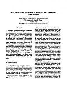
HH-EDA2 consists of two main phases: offline learning and online learning. In the offline learning phase, a number of masks to be used in the XOR generator are sampled over the search space. The search space is divided into M sub-spaces and a set of masks is generated randomly in each sub-space, thus making the masks distributed well over the landscape. For the XOR generator, each mask corresponds to a different environment. Then, for each environment (represented by each mask) PBIL is executed. As a result of this, good prob→ − ability vectors P list corresponding to a set of different environments are learned in an offline manner. These learned probability vectors are stored for later use during the online learning phase of HH-EDA2. In the online learning phase, the probability vectors − → P list, serve as the low-level heuristics, which a selection hyper-heuristic manages. Figure 1 shows a simple diagram illustrating the structure and execution of HHEDA2.

3 A Hybrid Framework for Dynamic Environments

Fig. 1 The framework of HH-EDA2

In this section, we describe our multi-phase hybrid framework, referred to as hyper-heuristic based dual population EDA (HH-EDA2), for solving dynamic environment problems. Our initial investigations in (Uluda˘g et al, 2012a,b) indicated that this framework has potential for solving dynamic environment problems. Therefore, in this paper, we extend our studies further and provide an analysis of this framework across a variety of dynamic environment problems with different change properties produced by the XOR dynamic problem generator and explore further enhancements and modifications. Although we chose PBIL2 as the EDA component in our studies, the proposed hybrid framework can combine any multi-population EDA with any selection hyperheuristic in order to exploit the strengths of both approaches.

The online learning phase of the HH-EDA2 framework uses the PBIL2 approach, explained in Section 2. Similar to PBIL2, the population is divided into two sub-populations and two probability vectors, one for each sub-population, are used simultaneously. As seen in Figure 1, pop1 represents the first sub-population − → and P 1 is its corresponding probability vector; pop2 − → represents the second sub-population and P 2 is its corresponding probability vector. HH Select shows selec− → tion of P 2 in Plist using heuristic selection methods. The pseudocode of the proposed HH-EDA2 is shown in Algorithm 1. − → In HH-EDA2, the first probability vector P 1 is ini− → tialized to P central , and the second probability vector − → P 2 is initialized to a randomly selected vector from − → P list. Initial sub-populations of equal sizes are sampled independently from their own probability vectors. Af-


Algorithm 1 Pseudocode of the proposed HH-EDA2 approach 1: 2: 3: 4: 5: 6: 7: 8: 9: 10: 11: 12: 13: 14: 15:

t := 0 − → − → initialize P 1 (0) := 0.5 − → − → P 2 (0) is selected from P list − → − → S1 (0) := sample( P 1 (0)) and S2 (0) := sample( P 2 (0)) while (termination criteria not fulfilled) do evaluate S1 (t) and evaluate S2 (t) − → − → adjust next population sizes for P 1 (t) and P 2 (t) respectively − → place k best samples from S1 (t) and S2 (t) into B (t) send best fitness from whole/second population to heuristic selection component − → − → learn P 1 (t) toward B (t) − → mutate P 1 (t) − → P 2 (t) is selected using heuristic selection − → − → S1 (t) := sample( P 1 (t)) and S2 (t) := sample( P 2 (t)) t := t + 1 end while

ter the fitness evaluation process, sub-population sample sizes are slightly adjusted within the range [0.3 ∗ n, 0.7∗n] according to their best fitness values. At each iteration, if the best candidate solution of the first subpopulation is better than the best candidate solution of the second sub-population, the sample size of the first sub-population, n1 is determined by min(n1 + 0.05 ∗ n, 0.7 ∗ n); otherwise n1 is defined by min(n1 − 0.05 ∗ − → n, 0.3 ∗ n). While, P 1 is learned towards the best solution candidate(s) in the whole population and mutation − → − → is applied to P 1 , P 2 is selected using the heuristic se→ − lection methods from P list. No mutation is applied to − → P 2 . Then, the two sub-populations are sampled based on their respective probability vectors. The approach repeats this cycle until some termination criteria are met. In the HH-EDA2 framework, different heuristic selection methods can be used for selecting the second → − probability vector from P list.

4 Experiments In this study, we performed four groups of experiments. In the first group, we investigated the influence of different heuristic selection methods on the performance of the proposed framework, to determine the most suitable one for dynamic environment problems. In the second group of experiments, the proposed framework, incorporating the chosen heuristic selection scheme, is compared to similar methods from literature. The third and fourth group of experiments focus on the offline and online learning components of the framework, respectively. We explore the influence of the time spent for offline learning on the performance of the overall approach. For the online learning component, we explore

7

the effects of the learning parameter on the overall performance and then propose and analyze an adaptive version.

4.1 Experimental Design and Settings In this subsection, we explain the dynamic environment problems used in the experiments and present the general parameter settings for all experiments. Moreover, approaches from literature that are implemented for comparisons and the details of their settings are also provided in this section. Further parameter settings specific to each experiment will be given in the relevant subsections. 4.1.1 Benchmark Problems and Settings of Algorithms We use three Decomposable Unitation-Based Functions (DUFs) Yang and Yao (2008) within the XOR generator. All Decomposable Unitation-Based Functions are composed of 25 copies of 4-bit building blocks. Each building block is denoted as a unitation-based function u(x) which gives the number of ones in the corresponding building block. Its maximum value is 4. The fitness of a bit string is calculated as the sum of the u(x) values of the building blocks. The optimum fitness value for all Decomposable Unitation-Based Functions is 100. DUF1 is the OneMax problem whose objective is to maximize the number of ones in a bit string. DUF2 has a unique optimal solution surrounded by four local optima and a wide plateau with eleven points having a fitness of zero. DUF2 is more difficult than DUF1. DUF3 is fully deceptive. The mathematical formulations of the Decomposable Unitation-Based Functions, as given in Yang and Yao (2008), can be seen below. fDU F 1 = u(x)   4 , if u(x) = 4 fDU F 2 = 2 , if u(x) = 3  0 , if u(x) < 3 { 4 , if u(x) = 4 fDU F 3 = 3 − u(x) , if u(x) < 4

(2) (3)

(4)

In the offline learning phase, first a set of M XOR masks are generated. In order to have the XOR masks distributed uniformly on the search space, an approach similar to stratified sampling is used. Then, for each mask, PBIL is executed for 100 independent runs where each run consists of G generations. During offline learning, each environment is stationary and 3 best candidate solutions are used to learn probability vectors. The population size is set to 100. At the end of the


8

offline learning stage, the probability vector producing the best solution found so far over all runs for each en− → vironment, is stored in P list. The parameter settings for PBIL used in this stage is given in Table 1 Table 1 Parameter settings for PBILs Parameter Solution length Population size Number of runs

Setting 100 100 100

Parameter Mutation rate Pm Mutation shift δm Learning rate α

Setting 0.02 0.05 0.25

After the offline learning stage, we experiment with four main types of dynamic environments: randomly changing environments (Random), environments with cyclic changes of type 1 (Cyclic1), environments with cyclic changes of type 1 with noise (Cyclic1-with-Noise) and environments with cyclic changes of type 2 (Cyclic2). In the Cyclic1 type environments, the masks representing the environments, which repeat in a cycle, are selected from among the sampled M masks used in the offline learning phase of HH-EDA2. To construct Cyclic1with-Noise type environments, we added a random bitwise noise to the masks used in the Cyclic1 type environments. In Cyclic2 type environments, the masks representing the environments, which repeat in a cycle, are generated randomly. To generate dynamic environments showing different dynamism properties, we consider different change frequencies τ , change severities ρ and cycle lengths CL. We determined the change periods which correspond to low frequency (LF), medium frequency (MF) and high frequency (HF) changes as a result of some preliminary experiments where we executed PBIL on stationary versions of all the Decomposable Unitation-Based Functions. The corresponding convergence plots for the Decomposable Unitation-Based Functions are given in Figure 4. As can be seen in the plots, the selected settings for low frequency, medium frequency and high frequency for each Decomposable Unitation-Based Function correspond respectively to stages where the PBIL algorithm has been converged for some time, where it has not yet fully converged and where it is very early on in the search. Table 2 shows the determined change periods for each Decomposable Unitation-Based Function. Table 2 The value of the change periods Functions DUF1 DUF2 DUF3

LF 50 50 100

MF 25 25 35

HF 5 5 10

In the Random type environments, the severity of changes are determined based on the definition of the XOR generator and are chosen as 0.1 for low severity (LS), 0.2 for medium severity (MS), 0.5 for high severity (HS), and 0.75 for very high severity (VHS) changes. For all types of cyclic environments, the cycle lengths CL are selected as 2, 4 and 8. Except for Cyclic1-withNoise type of environments, the environments return to their exact previous locations. In our previous study Uluda˘g et al (2012b), we explored the effects of restart schemes for HH-EDA2. Our experiments showed that a restart scheme significantly improves the performance of HH-EDA2. In the best performing restart scheme for HH-EDA2, only the first → − − → probability vector P 1 is reset to the to P central , whenever an environment change is detected. Since HH-EDA2 is a multi-population approach, which also uses a kind of memory, for our comparison experiments, we focused on memory based approaches as well as multi-population ones which were shown in literature to be successful in dynamic environments. Therefore, we used different variants of PBILs with restart schemes and a sentinel-based genetic algorithm. In Yang and Yao (2008), experiments show that a restart scheme combined with the multi-population PBIL, significantly outperforms dual population memorybased PBIL on most Decomposable Unitation-Based Functions in different kinds of dynamic environments. In the version of PBIL that utilizes a restart scheme − → − → (PBILr), the probability vector P is reset to P central when an environment change is detected. In the version of PBIL2 that utilizes a restart scheme (PBIL2r), whenever an environment change is detected, only the − → → − first probability vector P 1 is reset to P central . In the restart variant for memory-based PBIL (MPBILr), the − → − → probability vector P is reset to P central when change is detected. The parameter settings of memory-based PBIL with restart are the same as the PBIL used in the offline learning phase 1. In the dual population memory-based PBIL approach with a restart scheme (MPBIL2r), whenever an environment change is de− → tected, the second probability vector P 2 is reset to − → P central . The population size n is set to 100 and the memory size is fixed to 0.1∗n = 10. Initial sub-populations are 0.45 ∗ n = 45 and sub-population sample sizes are slightly adjusted within the range of [30, 60]. The memory is updated using a stochastic time pattern. After each memory update, the next memory updating time is set as tM = t + rand(5, 10). For the sentinel-based genetic algorithm, we used tournament selection where the tournament size is 2, uniform crossover with a probability of 1.0, mutation with a mutation rate of 1/l where l is the chromosome


9

length. The population size is set to 100. We tested two different values for the number of sentinels: 8 and 16. These values are chosen for two reasons. First of all, (Morrison, 2004) suggests working with 10% of the population as sentinels. Secondly, in our previous study, we experimented with storing M = 8 and M = 16 proba→ − bility vectors in P list for HH-EDA2 and found M = 8 to be better. At the beginning of the search, sentinels are initialized to locations of the masks representing different parts of the search space. For HH-EDA2, the masks used in the offline learning stage were chosen in such a way as to ensure that they are distributed uniformly on the search space. Therefore M = 8 or M = 16 masks are used as the sentinels. Both in PBIL2 and HH-EDA2, each sub-population size is initialized as 50 and adjusted within the range of [30, 70]. In Reinforcement Learning, score of each heuristic is initialized to 15 and is allowed to vary between 0 and 30. If the selected heuristic yields a solution with an improved fitness, its score is increased by 1, otherwise it is decreased by 1. The Reinforcement Learning settings ¨ are taken as recommended in Ozcan et al (2010). In (Kiraz et al, 2013b), the results show that Antbased Selection with roulette wheel selection is better than the version with tournament selection. Therefore, we work Ant-based Selection with roulette wheel selection in this paper. In (Kiraz et al, 2013b), ∆τ is calculated as ∆τ = 0.1 ∗ (1/fc ) so that pheromone values increase gradually. For Ant-based Selection, q0 and ρ are set to 0.5 and 0.1, respectively. These are the settings recommended in (Kiraz et al, 2013b). For each run of the algorithms, 128 changes occur after the initial environment. Therefore, the total number of generations in a run is calculated as maxGenerations = changeF requency ∗ changeCount. 4.1.2 Performance Evaluation Criteria In order to compare the performance of the algorithms, the results are reported in terms of offline error Branke (2002), which is calculated as the cumulative average of the differences between the best values found so far and the optimum value at each time step, as given below. T 1∑ | optt − et ∗ | T t=1

of each approach under a variety of change frequencyseverity pair settings in randomly changing environments and under different cycle length and change frequency settings in cyclic environments for three Decomposable Unitation-Based Functions. Each column shows the performance of all the approaches for the corresponding change frequency-severity pair settings in randomly changing environments and for the cycle length-change frequency pair settings in cyclic environments. In addition, in all the tables, the best performing approach(es) in each row is marked in bold. We also perform One-way ANOVA and Tukey HSD tests at a confidence level of 95% for testing whether the differences between the approaches are statistically significant or not. To provide a summary of the statistical comparison results, we count the number of times an approach obtains a significance state over the others on the three Decomposable Unitation-Based Functions for different change severity and frequency settings in randomly changing environments and for different cycle length and change frequency settings in cyclic environments. In the tables providing the summary of statistical comparisons, s+ shows the total number of times the corresponding approach performs statistically better than the others and s− shows the vice versa; ≥ shows the total number of times the corresponding approach performs slightly better than the others, however, the performance difference is not statistically significant and ≤ shows the vice versa. To compare the performance of approaches over different dynamic environments, the approaches are scored in the same way as in the CHeSC competition 1 . The scoring system in CHeSC is based on the Formula 1 scoring system used before 2010. For each approach, median, best and average values over 100 runs are calculated. Then, the results of the approaches are sorted with respect to these values. The top 8 approaches eventually get the following points for each problem instance: 10, 8, 6, 5, 4, 3, 2 and 1, respectively. The sum of scores over all problem instances is the final score of an algorithm. Considering random and cyclic environments, there are 117 problem instances, therefore, 1170 is the maximum overall score that an algorithm can get in this scoring system.

(5)

e∗t = max(eτ , eτ +1 , ..., et ) where T is the total number of evaluations and τ is the last time step (τ < t) when change occurred. In the result tables, each entry shows the average offline error values averaged over 100 independent runs. In the rows of the tables, we can see the performance

4.2 Results In this subsection, we provide and discuss the results of each group of experiments separately. 1

http://www.asap.cs.nott.ac.uk/external/chesc2011/


10

4.2.1 Comparison of heuristic selection methods

process. For example, the use of reinforcement learning in the selection hyper-heuristic (RL) yields the worst In this set of experiments, we test different heuristic average performance. Random Permutation as a nonselection methods within the proposed framework. The learning heuristic selection combines the learnt probtested heuristic selection methods are Simple Random ability vectors effectively yielding an improved perfor(SR), Random Descent (RD), Random Permutation (RP), mance which outperforms Simple Random. Random Permutation Descent (RPD), Reinforcement For randomly changing environments, all heuristic Learning (RL) and Ant-based Selection (AbS). We use selection schemes performed well and there were no all change frequency and severity settings for the Ranstatistically significant differences between the results. dom dynamic environments; we also use all change freThe results show that for DUF1 and DUF2, in the quency and cycle length settings for the Cyclic1, Cylic1tested cyclic environments, Random Permutation perwith-Noise and Cyclic2 type dynamic environments. Tests forms the best as a heuristic selection method in the are performed on all Decomposable Unitation-Based HH-EDA2 framework. For DUF3, Random PermutaFunctions, i.e. DUF1, DUF2 and DUF3. The results tion Descent seems to produce better results than Ranare summarized in Table 3 and 4. Table 3 provides the dom Permutation, however this performance difference statistical comparison summary, whereas Table 4 shows is not statistically significant and actual offline error the ranking results obtained based on median, best and values from Random Permutation are close to the ones average offline error values. produced by Random Permutation Descent. Due to space limitations, these results are omitted here. Table 3 Overall (s+, s−, ≥ and ≤) counts for the different heuristic selection schemes. Heuristic Selection RP RPD SR AbS RD RL

s+ 247 196 139 129 91 52

s− 58 68 123 173 181 251

≥ 192 122 197 148 144 98

≤ 88 199 126 135 169 184

Table 4 The overall score according to the Formula 1 ranking based on median, best and average offline error values for the different heuristic selection schemes. Heuristic Selection RP SR RPD AbS RD RL

Median 930 738 737 668 602 537

Best 908 706 767 626 626 579

Average 927 733 731 688 605 528

As seen in Table 3, Random Permutation generates the best average performance across all dynamic environment problems, performing significantly/slightly better than the rest for 247/192 instances. The second best approach is Random Permutation Descent on average. Random Permutation is still the best approach if the median and best performances are considered as well (Table 4) based on the Formula 1 ranking. It can be seen from the table that Random Permutation scores 930 and 908, respectively. Learning via the PBIL process helps, but using an additional learning mechanism on top of that turns out to be misleading for the search

4.2.2 Comparisons to selected approaches from literature In this set of experiments, we compare our approach to some well known and successful previously proposed approaches from literature as described in Section 4.1.1. As a result of the experiments in Subsection 4.2.1, we fixed the heuristic selection component as Random Permutation during these experiments and used the same problems, change settings and dynamic environment types as in Subsection 4.2.1. In a randomly changing environment, HH-EDA2 outperforms the rest of the previously proposed approaches on DUF1 and DUF2 regardless of the frequency or severity of the changes as illustrated in Tables 5 and 6, based on average offline error values, respectively. The same phenomenon is observed for DUF3, except for the low frequency cases (see Table 7). HH-EDA2 performs the best only when the changes occur at a low frequency and a very high severity on DUF3. On the other hand, sentinel-based genetic algorithm with 16 sentinels performs the best for the low and high severity change cases, while memory-based PBIL approaches with restart perform the best for the changes with medium severity on DUF3. In a cyclically changing environment of type 1 with and without noise, HH-EDA2 again outperforms the rest of the previously proposed approaches on DUF1 and DUF2 regardless of the cycle length or frequency of change as illustrated in Tables 8 and 9 based on average offline error values, respectively. For the Cyclic2 case, HH-EDA2 still performs the best on DUF1, except when the changes occur at a high frequency and


11

Table 5 Offline errors generated by different approaches averaged over 100 runs, on the DUF1 for different change severity and frequency settings in randomly changing environments. Algorithm HH-EDA2 PBILr PBIL2r MPBILr MPBIL2r Sentinel8 Sentinel16

LF LS

MS

HS

VHS

0.06 4.13 3.47 0.56 0.67 20.11 7.26

0.06 7.84 7.20 0.67 0.81 20.20 9.10

0.08 16.71 16.16 0.91 1.02 4.40 2.21

0.09 21.75 20.76 0.09 0.11 0.78 1.19

MF MS HS Random 0.17 0.25 0.86 9.51 16.24 26.68 9.04 15.80 25.95 1.84 2.21 2.78 4.85 4.30 4.32 22.84 23.00 11.83 12.35 15.10 12.42 LS

HF VHS

LS

MS

HS

VHS

0.99 30.44 29.14 1.29 2.83 9.21 12.36

21.94 27.91 27.56 26.88 26.98 28.29 24.36

23.60 33.91 33.32 28.66 29.70 29.43 27.56

26.79 38.02 37.23 30.33 31.52 32.12 31.91

28.26 38.76 38.11 30.41 31.60 33.91 33.57

Table 6 Offline errors generated by different approaches averaged over 100 runs, on the DUF2 for different change severity and frequency settings in randomly changing environments. Algorithm

HH-EDA2 PBILr PBIL2r MPBILr MPBIL2r Sentinel8 Sentinel16

LF LS

MS

HS

VHS

0.12 8.96 7.66 0.98 1.51 39.11 16.00

0.16 18.45 17.29 1.23 1.74 38.87 20.25

0.49 38.93 37.03 1.81 2.14 13.82 8.75

0.53 45.80 42.99 1.92 1.97 3.33 5.08

MF MS HS Random 0.43 0.85 4.13 20.58 34.65 51.43 19.51 33.58 49.67 4.81 5.48 6.78 12.28 10.50 10.40 43.52 42.72 27.69 25.71 30.43 28.11 LS

HF VHS

LS

MS

HS

VHS

4.54 54.83 52.67 7.07 10.61 23.73 28.38

42.92 52.69 51.55 51.11 51.50 51.33 45.78

45.74 60.41 59.38 53.81 55.02 52.93 50.67

50.86 65.11 64.05 55.77 57.46 57.52 57.41

52.95 65.70 64.46 56.25 57.94 59.64 59.49

Table 7 Offline errors generated by different approaches averaged over 100 runs, on the DUF3 for different change severity and frequency settings in randomly changing environments. Algorithm


LF LS

MS

HS

VHS

19.44 25.44 24.98 17.10 18.18 36.98 14.66

18.46 25.85 25.23 17.01 18.04 33.85 20.51

16.04 23.96 23.15 17.02 17.48 17.59 14.05

14.18 19.49 18.55 16.91 17.24 22.54 17.26

MF LS MS HS Random 19.75 18.99 17.26 30.06 33.11 35.27 29.38 32.42 34.37 19.20 19.26 19.34 24.07 23.18 21.60 40.04 36.56 26.88 31.04 31.22 30.94

the cycle length is low (2 and 4). For those problem instances, PBIL with restart approaches perform better. For DUF2 of type Cyclic2, HH-EDA2 is the best approach when the frequency of change is medium. HH-EDA2 delivers a poor performance on DUF3 for all cases, except for the high frequency cases for Cyclic1 with and without noise (see Table 10). The advantage of combining offline learning and online learning mechanisms disappear when the problem being solved is deceptive. The use of sentinels produces a better performance on DUF3 for a change type of Cyclic2. It should be noted that only for the sentinel-based genetic algorithm schemes and HH-EDA2, cyclic environments of type 1 and type 2 are different. In cyclic environments of type 1, the environment cycles between environments represented by the masks used in the of-

HF VHS

LS

MS

HS

VHS

15.49 31.56 30.73 19.04 21.87 28.13 27.82

38.44 40.11 39.55 44.67 41.18 43.07 38.94

39.99 44.48 43.66 45.78 44.93 41.79 42.76

41.29 47.18 46.41 46.28 46.49 43.88 46.20

40.75 45.85 45.07 46.08 45.82 41.74 45.59

fline learning stage. These masks are used as sentinels in the sentinel-based genetic algorithm schemes and the probability vectors obtained as a result of training on these masks are used as low level heuristics in HHEDA2. An overall comparison of all approaches are provided in Tables 11 and 12. HH-EDA2 generates the best average performance across all dynamic environment problems (Table 11) performing significantly/slightly better than the rest for 609/18 instances. The second best approach is memory-based PBIL using a single population and restart. Moreover, HH-EDA2 is the top approach if the median and best performances are considered as well (see Table 12) based on Formula 1 rankings, scoring 1035 and 998, respectively. The closest competitor accumulates a score of 711 and 639 for its


12

Table 8 Offline errors generated by different approaches averaged over 100 runs, on the DUF1 for different cycle length and change frequency settings in different cyclic dynamic environments. CL=2

LF CL=4


0.03 11.96 10.65 0.08 0.12 2.54 9.04

0.02 14.69 13.78 0.08 0.11 6.02 1.33


0.02 11.93 10.64 0.08 0.12 2.49 9.05

0.02 14.59 13.78 0.08 0.11 5.97 1.35


0.08 11.67 10.44 0.08 0.12 0.50 1.17

0.08 15.75 14.94 0.08 0.11 4.79 1.31

Algorithm

MF CL=2 CL=4 Cyclic1 0.02 0.05 0.04 17.09 15.47 19.11 16.53 12.10 17.76 1.76 1.30 1.29 1.98 3.98 3.36 4.94 19.02 14.05 3.55 14.81 11.96 Cyclic1-with-Noise 0.02 0.05 0.04 17.06 15.50 19.09 16.48 12.03 17.75 1.76 1.29 1.29 1.98 3.97 3.36 4.93 19.11 13.97 3.59 14.80 11.92 Cyclic2 0.08 0.85 0.86 17.18 15.16 21.39 16.63 11.91 20.03 0.08 1.30 1.29 0.11 4.03 3.03 5.11 19.89 17.65 1.73 14.70 12.08

CL=8

CL=8

CL=2

HF CL=4

CL=8

0.05 25.64 24.54 4.59 6.18 10.19 13.19

14.20 18.73 19.02 30.42 19.85 23.30 19.37

13.82 20.59 20.44 30.39 21.61 24.21 33.08

14.59 28.65 28.43 30.30 29.53 31.88 32.96

0.05 25.70 24.52 4.59 6.16 10.18 13.24

14.48 18.69 19.12 30.40 19.99 23.23 19.37

13.86 20.57 20.51 30.40 21.50 24.11 33.05

14.66 28.54 28.41 30.29 29.47 31.93 32.93

0.89 25.60 24.36 1.30 2.83 11.81 12.36

25.83 18.39 18.82 30.39 19.54 25.38 22.11

26.80 24.77 24.63 30.40 25.88 28.02 33.36

26.98 30.15 29.85 30.43 30.55 33.17 33.34


LF CL=4


0.04 23.57 19.97 0.23 0.51 33.16 21.11

0.04 32.85 30.46 14.39 11.68 15.29 6.21


0.04 23.56 19.89 0.24 0.53 33.12 21.16

0.04 32.79 30.42 14.38 11.74 15.61 6.24


0.45 24.00 20.20 0.25 0.51 4.79 5.04

0.46 34.29 32.08 0.24 0.39 12.58 5.81

Algorithm


CL=8

CL=8

CL=2

HF CL=4

CL=8

0.08 47.93 45.52 11.89 14.95 23.56 28.85

27.33 29.92 30.76 55.93 32.37 39.09 35.43

27.38 38.36 38.50 55.31 39.73 46.03 58.80

26.53 50.70 50.45 55.35 51.32 57.70 59.14

0.09 47.94 45.64 11.96 14.88 23.58 28.78

26.96 29.63 30.79 55.97 32.57 39.27 35.36

26.37 38.33 38.54 55.33 39.81 45.97 58.79

27.34 50.66 50.35 55.36 51.39 57.65 59.11

4.25 49.84 47.46 7.36 10.87 27.94 28.38

49.34 30.39 31.04 55.95 32.74 41.23 39.86

50.82 43.54 43.69 55.92 45.69 51.41 59.35

51.20 53.57 53.02 55.62 53.97 58.90 59.36


13


LF CL=4


10.09 24.11 23.37 16.76 17.54 2.51 3.21

11.36 24.34 23.60 16.79 17.25 2.19 3.38


10.09 24.05 23.40 16.81 17.50 2.49 3.17

11.35 24.38 23.62 16.78 17.23 2.20 3.39


16.27 24.86 24.10 16.80 17.32 2.27 3.36

16.60 24.61 23.86 16.80 17.27 2.24 3.58

Algorithm


CL=8

median and best performances, respectively. These results also indicate that the use of a dual population and the selection hyper-heuristic both improves the performance of the overall algorithm. Table 11 Overall (s+, s−, ≥ and ≤) counts for the algorithms used Algorithm HH-EDA2 MPBILr MPBIL2r Sentinel16 Sentinel8 PBIL2r PBILr

s+ 609 390 367 335 298 236 132

s− 72 278 297 346 384 442 548

≥ 18 20 7 5 15 14 11

≤ 3 14 31 16 5 10 11

4.2.3 Duration of offline learning In this set of experiments, we look into the effect of the offline learning phase. In normal operation, for each problem (DUF1, DUF2 and DUF3 in this paper), before running the algorithm we execute an offline learning phase. In the XORing generator, each different environment is represented with an XOR mask which is applied to the solution candidate during fitness evaluations. We sample the space of the XOR masks, gener-

CL=8

CL=2

HF CL=4

CL=8

11.58 33.94 33.02 18.88 21.45 9.05 11.04

22.23 26.72 26.43 46.64 27.67 24.22 24.78

22.42 37.40 36.52 46.63 38.32 24.87 24.95

22.76 41.63 40.57 46.59 42.24 24.91 24.93

11.59 33.91 33.00 18.86 21.45 9.11 10.94

22.21 26.71 26.35 46.62 28.13 24.30 24.74

23.20 37.61 36.38 46.70 38.21 24.89 24.95

23.20 41.54 40.53 46.60 42.23 24.90 24.93

17.24 35.22 34.34 19.85 21.96 7.80 11.10

40.67 27.22 27.03 46.69 28.31 24.80 24.89

41.19 37.87 37.23 46.67 38.60 24.90 24.96

41.34 42.89 41.72 45.78 43.25 24.90 24.95

Table 12 The overall score according to the Formula 1 ranking based on median, best and average offline error values for the algorithms used Algorithm HH-EDA2 MPBILr MPBIL2r Sentinel16 Sentinel8 PBIL2r PBILr

Median 1035 711 608 606 598 498 390

Best 998 639 812 581 583 468 365

Average 1035 709 611 606 598 497 390

ating M of them which are distributed uniformly over the landscape. Then for each environment, represented by each mask, we train an PBIL algorithm for G iterations to learn a good probability vector for that environment. In this set of experiments, we explore the effect of the number of iterations G performed during the offline learning stage. In the experiments we choose M = 8 masks to represent 8 environments. We train PBIL for various the number of iteration G settings as: G = {0, 1, 5, 10, 20, 25, 30, 40, 50, 75, 100, 150, 200, 250,500, 1000, 10000}. Then, we execute HH-EDA2 incorporating the Random Permutation heuristic selection, using the set of probability vectors created by each the number of iteration G setting and record the final offline errors. For these experiments, we use all change

14

frequency and severity settings for the Random type dynamic environments; we also use all change frequency and cycle length settings for the Cyclic1 and Cyclic1with-Noise type dynamic environments. The tests are performed using DUF1, DUF2 and DUF3. If the number of iteration G is 0, then this indicates that there is no offline learning. Although offline learning improves the performance of the overall algorithm slightly for any given problem, the value of the number of iteration G does not matter much if the environment changes randomly. Figure 2 illustrates this phenomenon on the Decomposable Unitation-Based Functions for medium frequency and medium severity changes (MFMS). We can observe that small G values is sufficient to handle any type of dynamic environment. Figure 3 illustrates that the number of iteration G should be set larger than or equal to 20 for an improved performance to solve DUF1 and DUF2 when the frequency of change is medium, the type is Cyclic1 and the cycle length is 4, while the choice of values greater than 50 for the number of iteration G is sufficient on DUF3. Due to lack of space, the plots for other dynamic environment instances are not provided here, however, similar observations were made for those cases too. Figure 4 illustrates the convergence behavior of PBIL on the stationary versions of the Decomposable UnitationBased Functions. The frequency levels corresponding to low frequency, medium frequency and high frequency were determined using these plots. It is interesting to note that the values of the number of iteration G which are seen to be sufficient for good performance, approximately coincide with our medium frequency settings for the different Decomposable Unitation-Based Functions. This shows that, since for random type changes, the value of the number of iteration G does not make a difference, to achieve a good level of performance, offline learning should be done until PBIL partially converges. This will provide a heuristic way to determine a good the number of iteration G value for other types of problems encountered in the future. 4.2.4 Adaptive online learning and mutation rates During the tests in Uluda˘g et al (2012b), we experimented with different learning rates α and mutation rates Pm . The experiments showed that the selection of these rates are important for algorithm performance. According to our experiments, a good value for learning rate α is 0.1 and for Pm is 0.35 for the tested dynamic environment problems. To be able to decrease the number of parameters needing to be tuned, thus making our approach more general, here we propose adaptive versions for the mutation rate parameter and the learning


rate parameter. We use the same adaptive approach for both parameters as given in Equation 6 and Equation 7.  t−1 , if ∆E < 0  βα αt = αt−1 , if ∆E = 0 (6)  1 t−1 α , if ∆E > 0 β where, E t is the error value for the generation t. ∆E = E t − E t−1 is the difference between the current and the former error value. β is the learning factor and γ is the mutation factor. The lower and upper bounds of the interval for learning rate α is chosen as 0.25 ≤ α ≤ 0.75 and for mutation rate Pm as 0.05 ≤ Pm ≤ 0.3.  t−1 , if ∆E < 0  γPm t−1 t , if ∆E = 0 Pm = Pm (7) 1 t−1 , if ∆E > 0 γ Pm The initial values of these parameters (t = 0) are 0 chosen as α0 = 0.75 and Pm = 0.3. Throughout the generations, if the values become less than the lower bound or greater than the upper bound, learning rate α and mutation rate Pm are reset to their tuned values (α = 0.35, Pm = 0.1), found in our previous study Uluda˘g et al (2012b). To see the effects of adaptive learning rate α and adaptive mutation rate Pm separately, we perform the same set of experiments three times: with only adaptive α and fixed mutation rate Pm ; with only adaptive mutation rate Pm and fixed learning rate α; with both adaptive learning rate α and mutation rate Pm . For the first set, we fixed the mutation rate value to Pm = 0.1. For the second set, we fixed the learning rate value to α = 0.35. For the third set, both parameters are allowed to vary between their predetermined lower and upper bounds. For the learning factor β and the mutation factor γ, we experimented with various setting combinations between 0.8 and 0.99 and we chose an acceptable one as being β = 0.99 and γ = 0.99. We did not perform extensive experiments to set these parameters, since we did not want to fine tune too much, as this would contradict our initial aim of trying to decrease the amount of fine tuning required. Besides, our results showed that the settings for these parameters are not very sensitive. For this experiment also, we used the same problems, change settings and dynamic environment types as those used in Subsection 4.2.3. The results of these experiments are provided in Tables 13 and 14. The results in Table 13 and Table 14 show that having only one of the parameters as adaptive decreases solution quality. However, the cases where both parameters are adaptive, produces results which are equivalent to those obtained when the parameters are fixed


15

0.3

1

19.6

19.5

0.29 0.95

19.4

0.28

19.3

0.26

0.25

0.24

Offline Error

0.9

Offline Error

Offline Error

0.27

0.85

19.2

19.1

19

0.8 18.9

0.23

18.8 0.75

0.22

18.7

0.21

0

1

5

10

20

25

30

40

50

75

0.7

100 150 250 500 100010000

0

1

5

10

20

(a) DUF1

25

30

40

50

75

18.6

100 150 250 500 100010000

0

1

5

10

20

(b) DUF2

25

30

40

50

75

100 150 250 500 100010000

(c) DUF3

Fig. 2 Error bar of different the number of iteration G settings for all Decomposable Unitation-Based Functions in random environment 1

4.5

19

0.9

4

18

3.5

17

3

16

0.8

0.6

0.5

0.4

Offline Error

Offline Error

Offline Error

0.7

2.5

2

15

14

1.5

13

1

12

0.1

0.5

11

0

0

0.3

0.2

0

1

5

10

20

25

30

40

50

75

100 150 250 500 100010000

0

1

5

10

(a) DUF1

20

25

30

40

50

75

100 150 250 500 100010000

10

0

1

5

10

(b) DUF2

20

25

30

40

50

75

100 150 250 500 100010000

(c) DUF3

Fig. 3 Error bar of different the number of iteration G settings for all Decomposable Unitation-Based Functions in cyclic environment

90 80 70 60 50 40

90 80 70 60 50 40

30

30

20

20 0

20

40

60

80

100 120 140

Number of generations

(a) DUF1

110

DUF2

100 Mean Best Fitness

Mean Best Fitness

110

DUF1

100

DUF3

100 Mean Best Fitness

110

90 80 70 60 50 40 30 20

0

20

40

60

80

100 120 140


(b) DUF2

0

20

40

60

80

100 120 140


(c) DUF3

Fig. 4 Convergence of mean (100 runs) of best fitness in each generation for all Decomposable Unitation-Based Functions

as a result of initial fine tuning experiments. This observation fails for high frequency change cases both for random and cyclic type of environments. The mutation rate Pm value is set initially to its upper bound value. Since the stationary periods between the changes is very short in the high frequency cases, with a decrease rate of γ = 0.99, the mutation rate Pm value does not decrease much before the environment changes and the solution quality drops, causing an increase in the mutation rate Pm value. A higher mutation rate seems to help in high frequency change cases. This needs to be further explored. However, overall, the results shows that an adaptive learning rate α and an adaptive mu-

tation rate Pm approach can be used within HH-EDA2 without performance loss. 5 Conclusion and Future Work In this study, we investigated the performance of a framework which enables hybridization of EDAs and selection hyper-heuristics based on online and offline learning mechanisms for solving dynamic environment problems (Uluda˘g et al, 2012a). A dual population approach is implemented, referred to as HH-EDA2 which uses PBIL as the EDA. The performance of the overall algorithm is tested using different heuristic selection methods to determine the best one for HH-EDA2. The


16

Table 13 Offline errors generated by HH-EDA2 using the tuned α = 0.35, Pm = 0.1 settings and HH-PBIL2 with the various adaptive schemes for α and Pm , averaged over 100 runs, on the three Decomposable Unitation-Based Functions for different change severity and frequency settings in randomly changing environments. Algorithm

LF LS

MS

HS

VHS

Tuned Adp. α & Pm Adp. α Adp. Pm

0.06 0.06 0.91 0.07

0.06 0.06 0.95 0.12

0.08 0.08 1.03 0.38

0.09 0.09 1.05 0.41


0.12 0.13 1.89 0.28

0.16 0.16 1.99 1.04

0.49 0.49 2.30 7.15

0.53 0.53 2.35 7.29


19.44 19.46 19.77 22.12

18.46 18.39 19.30 20.93

16.04 16.10 17.90 16.81

14.18 14.17 16.56 14.09

MF LS MS HS DUF1 0.17 0.25 0.86 0.17 0.26 0.85 2.85 3.19 4.20 0.52 1.29 4.02 DUF2 0.43 0.85 4.13 0.43 0.84 4.12 6.30 7.22 10.43 1.36 4.27 15.54 DUF3 19.75 18.99 17.26 19.77 18.98 17.29 22.86 23.04 23.04 22.44 21.46 18.30

HF VHS

LS

MS

HS

VHS

0.99 0.98 4.42 4.27

21.94 21.92 23.67 7.68

23.60 23.64 25.04 13.96

26.79 26.77 27.45 23.85

28.26 28.24 28.70 25.99

4.54 4.53 10.99 16.20

42.92 42.87 45.70 16.33

45.74 45.74 47.95 29.14

50.86 50.83 51.87 45.20

52.95 52.88 53.64 48.23

15.49 15.50 22.11 15.62

38.44 38.44 42.49 24.47

39.99 39.98 43.43 26.53

41.29 41.33 44.13 27.97

40.75 40.70 43.85 25.50

Table 14 Offline errors generated by HH-EDA2 using the tuned α = 0.35, Pm = 0.1 settings and HH-EDA2 with the various adaptive schemes for α and Pm , averaged over 100 runs, on the three Decomposable Unitation-Based Functions for different change severity and frequency settings in cyclic environments of type 1 (Cyclic1). CL=2

LF CL=4

CL=8


0.03 0.03 0.43 0.02

0.02 0.02 0.26 0.02

0.02 0.02 0.33 0.02


0.04 0.04 0.54 0.04

0.04 0.04 0.51 0.04

0.04 0.04 0.62 0.04


10.09 10.10 11.11 10.06

11.36 11.36 11.99 11.26

11.33 11.33 12.07 11.26

Algorithm

CL=2 DUF1 0.05 0.05 0.95 0.05 DUF2 0.09 0.09 1.33 0.08 DUF3 10.35 10.35 12.25 10.23

results revealed that, contrary to our initial intuition, the heuristic selection mechanism with learning isn’t the most successful one for the HH-EDA2 framework. The selection scheme that relies on a fixed permutation of the underlying low-level heuristics (Random Permutation) is the most successful one. For the cases when the change period is long enough to allow all the vectors in the permutation to be applied at least once, the Random Permutation heuristic selection mechanism becomes equivalent to Greedy Selection. In HH-EDA2, the move acceptance stage of a hyper-heuristic is not used. This is the same as using the Accept All Moves strategy. This move acceptance scheme is known to perform

MF CL=4

CL=8

CL=2

HF CL=4

CL=8

0.04 0.05 0.61 0.04

0.05 0.05 0.77 0.04

14.20 14.20 14.58 8.07

13.82 13.47 14.48 7.76

14.59 14.01 15.60 7.72

0.08 0.08 1.27 0.08

0.08 0.09 1.50 0.07

27.33 26.63 27.92 14.37

27.38 28.48 28.44 14.13

26.53 27.13 28.70 14.66

11.60 11.61 12.72 11.38

11.58 11.57 12.96 11.37

22.23 22.34 24.26 12.39

22.42 22.49 23.97 13.07

22.76 23.01 24.03 13.21

the best with the Greedy Selection method Kiraz et al (2011). HH-EDA2 is in general capable of adapting itself to the changes rapidly whether the change is random or cyclic. Even though the hybrid method provides good performance in the overall, it generates an outstanding performance particularly in cyclic environments. This is somewhat expected, since the hybridization technique based on a dual population acts similar to a memory scheme, which is already known to be successful in cyclic dynamic environments Yang and Yao (2008). The use of offline learning and then the us of online learning mechanism works and provides sufficient amount of diversification needed during the search process even un-


der different change dynamics. The overall performance of the algorithm worsens if the offline learning phase is ignored. HH-EDA2 outperforms well know approaches from the literature for almost all cases, except for some deceptive problems. As future work, we will experiment with the other types of more complex EDA based methods, in particular Bayesian optimization algorithm within the proposed framework. We will also verify our findings in a real-world problem domain, for example the dynamic vehicle routing problem.

A Appendix Table 15 summarizes the list of abbreviations used mostly in the paper.

Table 15 List of Abbreviations EDA PBIL PBIL2 HH-EDA2 PBILr PBIL2r MPBILr MPBIL2r Sentinel8 Sentinel16 LF MF HF LS MS HS VHS CL

Estimation of Distribution Algorithms Population Based Incremental Learning Dual Population PBIL Hyper-heuristic Based Dual Population EDA PBIL with restart PBIL2 with restart Memory-based PBIL with restart Dual Population Memory-based PBIL with restart Sentinel-based Genetic Algorithm with 8 sentinels Sentinel-based Genetic Algorithm with 16 sentinels Low Frequency Medium Frequency High Frequency Low Severity Medium Severity High Severity Very High Severity Cycle Length

Acknowledgements This work is supported in part by the EPSRC, grant EP/F033214/1 (The LANCS Initiative Postdoctoral Training Scheme) and Berna Kiraz is supported by the TUBITAK 2211-National Scholarship Programme for PhD students.

References Baluja S (1994) Population-based incremental learning: A method for integrating genetic search based function optimization and competitive learning. Tech. rep., Computer Science Department, Carnegie Mellon University, Pittsburgh, PA, USA Barlow GJ, Smith SF (2009) Using memory models to improve adaptive efficiency in dynamic problems. In: IEEE Symposium on Computational Intelligence in Scheduling, , CISCHED, p 714 Bosman PAN (2005) Learning, anticipation and timedeception in evolutionary online dynamic optimization. In: Proc. of the 2005 workshops on genetic and evolutionary computation, ACM, GECCO ’05, pp 39–47 Branke J (1999) Memory enhanced evolutionary algorithms for changing optimization problems. In: In Congress on

17 Evolutionary Computation CEC 99, IEEE, vol 3, pp 1875– 1882 Branke J (2002) Evolutionary optimization in dynamic environments. Kluwer Branke J, Kauler T, Schmidt C, Schmeck H (2000) A multipopulation approach to dynamic optimization problems. In: 4th Int. Conference on Adaptive Computing in Design and Manufacture (ACDM 2000), Springer, pp 299–308 Burke E, Kendall G (eds) (2005) Search Methodologies: Introductory Tutorials in Optimization and Decision Support Techniques. Springer Burke EK, Gendreau M, Hyde MR, Kendall G, Ochoa G, ¨ Ozcan E, Qu R (2012) Hyper-heuristics: A survey of the state of the art. to appear in the Journal of the Operational Research Society Cao Y, Luo W (2010) A novel updating strategy for associative memory scheme in cyclic dynamic environments. In: Advanced Computational Intelligence (IWACI), 2010 3rd Int. Workshop on, Suzhou, Jiangsu, pp 32–39 Chakhlevitch K, Cowling P (2008) Hyperheuristics: Recent developments. In: Cotta C, Sevaux M, Sirensen K (eds) Adaptive and Multilevel Metaheuristics, Studies in Computational Intelligence, vol 136, Springer, pp 3–29 Cowling PI, Kendall G, Soubeiga E (2000) A hyper-heuristic approach to scheduling a sales summit. In: Practice and Theory of Automated Timetabling III : 3rd Int. Conference, PATAT 2000, Springer, LNCS, vol 2079 Cruz C, Gonzalez J, Pelta D (2011) Optimization in dynamic environments: a survey on problems, methods and measures. Soft Computing - A Fusion of Foundations, Methodologies and Applications 15:1427–1448 Fernandes CM, Lima C, Rosa AC (2008a) Umdas for dynamic optimization problems. In: Proc. of the 10th conference on genetic and evolutionary computation, ACM, GECCO ’08, pp 399–406 Fernandes CM, Lima C, Rosa AC (2008b) Umdas for dynamic optimization problems. In: Proceedings of the 10th annual conference on Genetic and evolutionary computation, ACM, New York, NY, USA, GECCO ’08, pp 399–406 Ghosh A, Muehlenbein H (2004) Univariate marginal distribution algorithms for non-stationary optimization problems. Int J Know-Based Intell Eng Syst 8(3):129–138 Goncalves AR, Zuben FJV (2011) Online learning in estimation of distribution algorithms for dynamic environments. In: IEEE Congress on Evolutionary Computation, IEEE, pp 62–69 Kiraz B, Topcuoglu HR (2010) Hyper-heuristic approaches for the dynamic generalized assignment problem. In: Intelligent Systems Design and Applications (ISDA), 2010 10th International Conference on, pp 1487–1492 ¨ Kiraz B, S ¸ ima Uyar, Ozcan E (2011) An investigation of selection hyper-heuristics in dynamic environments. In: Proc. of EvoApplications 2011, Springer, LNCS, vol 6624 ¨ Kiraz B, S ¸ ima Etaner-Uyar A, Ozcan E (2013a) Selection hyper-heuristics in dynamic environments. Journal of the Operational Research Society, to appear ¨ Kiraz B, S ¸ ima Uyar, Ozcan E (2013b) An ant-based selection hyper-heuristic for dynamic environments. In: EvoApplications 2013, Under review Kobliha M, Schwarz J, Oˇ cen´ aˇsek J (2006) Bayesian optimization algorithms for dynamic problems. In: EvoWorkshops, Springer, Lecture Notes in Computer Science, vol 3907, pp 800–804 Larra˜ naga P, Lozano JA (eds) (2002) Estimation of Distribution Algorithms: A New Tool for Evolutionary Computation. Kluwer, Boston, MA

18 Lewis J, Hart E, Ritchie G (1998) A comparison of dominance mechanisms and simple mutation on nonstationary problems. In: Proc. of Parallel Problem Solving from Nature, pp 139–148 Li X, Mabu S, Mainali M, Hirasawa K (2011) Probabilistic model building genetic network programming using multiple probability vectors. In: TENCON 2010 - IEEE Region 10 Conference, IEEE Region Conference, Fukuoka, pp 1398–1403 Morrison RW (2004) Designing evolutionary algorithms for dynamic environments. Springer Nareyek A (2004) Metaheuristics. Kluwer, pp 523–544 ¨ Ozcan E, Bilgin B, Korkmaz EE (2008) A comprehensive analysis of hyper-heuristics. Intelligent Data Analysis 12:3– 23 ¨ Ozcan E, Misir M, Ochoa G, Burke EK (2010) A reinforcement learning - great-deluge hyper-heuristic for examination timetabling. International Journal of Applied Metaheuristic Computing 1(1):39–59 Peng X, Gao X, Yang S (2011) Environment identificationbased memory scheme for estimation of distribution algorithms in dynamic environments. Soft Comput 15:311–326 Ross P (2005) Hyper-heuristics. In: Burke EK, Kendall G (eds) Search Methodologies: Introductory Tutorials in Optimization and Decision Support Techniques, Springer, chap 17, pp 529–556 Shakya S, Oliveira F, Owusu G (2007) An application of eda and ga to dynamic pricing. In: Proc. of the 9th annual conference on Genetic and evolutionary computation, New York, NY, USA, GECCO ’07, pp 585–592 Sim˜ oes A, Costa E (2008a) Evolutionary algorithms for dynamic environments: Prediction using linear regression and markov chains. In: Proceedings of the 10th international conference on Parallel Problem Solving from Nature: PPSN X, Springer-Verlag, Berlin, Heidelberg, pp 306–315 Sim˜ oes A, Costa E (2008b) Evolutionary algorithms for dynamic environments: Prediction using linear regression and markov chains. Tech. rep., Coimbra, Portugal Sim˜ oes A, Costa E (2009a) Improving prediction in evolutionary algorithms for dynamic environments. In: Proceedings of the 11th Annual conference on Genetic and evolutionary computation, ACM, New York, NY, USA, GECCO ’09 Sim˜ oes A, Costa E (2009b) Prediction in evolutionary algorithms for dynamic environments using markov chains and nonlinear regression. In: Proceedings of the 11th Annual conference on Genetic and evolutionary computation, ACM, New York, NY, USA, GECCO ’09, pp 883–890 ¨ Uluda˘ g G, Kiraz B, S ¸ ima Etaner Uyar A, Ozcan E (2012a) A framework to hybridise PBIL and a hyper-heuristic for dynamic environments. In: PPSN 2012: 12th International Conference on Parallel Problem Solving from Nature, Springer, vol 7492, pp 358–367 ¨ Uluda˘ g G, Kiraz B, S ¸ ima Etaner Uyar A, Ozcan E (2012b) Heuristic selection in a multi-phase hybrid approach for dynamic environments. In: 12th UK Workshop on Computational Intelligence, Edinburgh, Scotland, UKCI12 Ursem RK (2000) Multinational GA optimization techniques in dynamic environments. In: Proc. of the Genetic Evol. Comput. Conf., pp 19–26 Uyar c, Harmanci E (2005) A new population based adaptive domination change mechanism for diploid genetic algorithms in dynamic environments. Soft Comput 9(11):803– 814 Wineberg M, Oppacher F (2000) Enhancing the GA’s Ability to Cope with Dynamic Environments. In: Whitley (ed) Genetic and Evolutionary Computation Conference, Morgan

¨ Uluda˘ g,Kiraz,Etaner-Uyar,Ozcan Kaufmann, pp 3–10 Wu Y, Wang Y, Liu X (2010a) Multi-population based univariate marginal distribution algorithm for dynamic optimization problems. Journal of Intelligent and Robotic Systems 59(2):127–144 Wu Y, Wang Y, Liu X, Ye J (2010b) Multi-population and diffusion umda for dynamic multimodal problems. Journal of Systems Engineering and Electronics 21(5):777–783 Xingguang P, Demin X, Fubin Z (2011) On the effect of environment-triggered population diversity compensation methods for memory enhanced umda. In: Proc. of the 30th Chinese Control Conference, pp 5430–5435 Yang S (2004) Constructing dynamic test environments for genetic algorithms based on problem difficulty. In: In Proc. of the 2004 Congress on Evolutionary Computation, pp 1262–1269 Yang S (2005a) Memory-enhanced univariate marginal distribution algorithms for dynamic optimization problems. In: Proc. of the 2005 Congress on Evol. Comput, pp 2560–2567 Yang S (2005b) Population-based incremental learning with memory scheme for changing environments. In: Proceedings of the 2005 conference on Genetic and evolutionary computation, ACM, New York, NY, USA, GECCO ’05, pp 711–718 Yang S (2007) Explicit Memory Schemes for Evolutionary Algorithms in Dynamic Environments. In: Evolutionary Computation in Dynamic and Uncertain Environments, chap 1, pp 3–28 Yang S, Richter H (2009) Hyper-learning for populationbased incremental learning in dynamic environments. In: in Proc. 2009 Congr. Evol. Comput, pp 682–689 Yang S, Yao X (2005) Experimental study on populationbased incremental learning algorithms for dynamic optimization problems. Soft Comput 9(11):815–834 Yang S, Yao X (2008) Population-based incremental learning with associative memory for dynamic environments. IEEE Trans on Evolutionary Comp 12:542–561 Yang S, Ong YS, Jin Y (eds) (2007) Evolutionary Computation in Dynamic and Uncertain Environments, Studies in Computational Int., vol 51. Springer Yaochu J, Branke J (2005) Evolutionary optimization in uncertain environments-a survey. IEEE Trans on Evolutionary Comp 9(3):303–317 Yuan B, Orlowska ME, Sadiq SW (2008) Extending a class of continuous estimation of distribution algorithms to dynamic problems. Optimization Letters 2(3):433–443

A Hybrid Multi-population Framework for Dynamic Environments ...

A Hybrid Multi-population Framework for Dynamic Environments ...

Suggest Documents

A Dynamic Web Service Registry Framework for Mobile Environments

DIT - University of Trento A FRAMEWORK FOR DYNAMIC HYBRID

A Dynamic Hybrid Framework for Constrained Evolutionary Optimization

A Hybrid, Dynamic Logic for Hybrid-Dynamic Information Flow

A Framework for Designing Collaborative Learning Environments

SoCQ: a Framework for Pervasive Environments - CNRS

A conceptual framework for ubiquitous mobile environments.

A Framework for Ontology-based Authoring Environments

A Framework for Mobile Collaborative Environments - CiteSeerX

A Framework for Designing 3D Virtual Environments

An Optimization Framework for Dynamic Hybrid Energy Systems

A Competitive Multipopulation Evolutionary Algorithm for Ship

An Optimization Framework for Dynamic Hybrid Energy Systems

Hybrid Learning Environments - OECD.org

A Framework for Hybrid Intrusion Detection Systems

A hybrid analysis framework for detecting web

A Hybrid Systems Modeling Framework for

Hybrid Learning Environments - OECD

A Framework for Hybrid Warfare: Threats, Challenges

A Framework for Solving Hybrid Influence

An authentication framework for a hybrid satellite

A Hybrid System Framework for Unified Impedance

A hybrid business model framework for IoT

Service-oriented Middleware for Hybrid Environments