A Hybrid Systems Modeling Framework for Embedded Computing Ricardo G. Sanfelice
CCDC, Department of ECE, University of California, Santa Barbara, California.
[email protected]
Ryan Kastner
Department of ECE, University of California, Santa Barbara, California.
[email protected]
ABSTRACT Hybrid systems define a modeling framework with interacting continuous-time and discrete-time dynamics that arise in many engineering applications. Embedded computing systems are naturally represented as hybrid systems using discrete model(s) for the digital components and continuous model(s) for the environment and analog components. We propose a general model for embedded systems that is based on the theory of hybrid systems. This establishes a mathematical structure for the systematic analysis, robust design, and simulation of real-time embedded systems. Our framework contains independent models for the environment and the components of the digital system. We describe how several common models for embedded computing easily fit within the framework. We illustrate the modeling ideas by examples.
Keywords embedded systems modeling, embedded computing, hybrid systems
1. INTRODUCTION Computing devices have permeated our lives. They aid our transportation (luxury cars contain close to 100 microprocessors), communication (digital signal processors are the core of every cell phone) and physical well being (microcontrollers run pacemakers, hearing aids, etc.). These embedded computers differ significantly from traditional desktop computers. They constitute a portion of a larger object that often is not considered a computer. They are rarely controlled through a keyboard, mouse and display; rather they interface with sensors, actuators, antennas and other peripherals that connect to a physical environment. They frequently work autonomously and interact with an environment that is not well defined or precisely specified. Failure of such systems may cause serious harm. All of this
Research partially supported by the Army Research Office under Grant no. DAAD19-03-1-0144, the National Science Foundation under Grant no. CCR-0311084 and Grant no. ECS-0324679, and by the Air Force Office of Scientific Research under Grant no. F49620-03-1-0203.
Andrew R. Teel
CCDC, Department of ECE University of California, Santa Barbara, California.
[email protected]
makes the modeling and design of embedded systems an extremely difficult, yet immensely important problem. We consider embedded systems as the combination of an environment with digital systems for a particular application. In our model, the digital systems interact with the environment (e.g. a human operator, a communication channel, a device to be controlled, etc.) and consist of embedded computers (e.g. general purpose processors, microcontrollers, digital signal processors) and analog-to-digital/ digital-to-analog converters (or equivalently, sample and hold devices). This structural definition of embedded systems is depicted in Figure 1. To solidify the understanding of our model, consider the following applications: • Digital communication system: the environment consists of the communication channel, wired or wireless, between transmitters and receivers while the digital system is given by analog-to-digital (ADC) and digital-to-analog (DAC) converters that translate the information between the communication channel, and the transmitters and receivers that are implemented in the embedded computer. • Embedded control system: the environment consists of a controllable system including analog sensors and actuators, while the digital system is given by ADC and DAC converters, which provide the interface between the environment and an embedded computer. The computer runs a control algorithm that processes the samples of the environment and transforms the environment through the DAC converters connected to actuators. • Sensor network: the environment consists of the links between the nodes of the sensors in the network while the digital system is given by the ADC and DAC converters and the embedded computers in each node implementing the sensing communication protocol. Models of computation [16] are often used as a framework for understanding, simulating, and reasoning about an embedded system. Models of computation govern the interaction between the modules of an embedded system. In other words, they define the semantics of the composition of the modules in these systems. The composition of digital systems with the surrounding environment that arises in embedded systems can be also interpreted as a hybrid system [1],[13]. Hybrid systems are dynamical systems with interacting continuous-time and
discrete-time dynamics. In hybrid systems, the continuoustime dynamics define the “flows” of the hybrid system, while the discrete-time dynamics define the “jumps” (or discrete transitions). For general hybrid systems, the flows are modeled by differential equations (or inclusions) and the jumps are modeled by difference equations (or inclusions); both are enabled when the state of the hybrid system satisfies certain conditions. Embedded systems can be modeled with the hybrid system framework: the continuous-time dynamics of the hybrid system model the dynamics of the analog devices, and the discrete-time dynamics model the dynamics of the digital devices in an embedded system.
Figure 1: Components of an embedded system: the environment and the digital system. The analog-todigital/digital-to-analog converters (ADC/DAC) and the embedded computer conform the digital system. In this paper, we propose a hybrid system model for embedded systems that defines a formal mathematical framework for the analysis, design, and simulation of embedded systems. This allows us to import the theory of hybrid systems, which can address important problems in the area of embedded systems like design of controllers with unmodeled dynamics, time delays, and quantization, among others. Here, we take a first step in this direction by introducing a hybrid system model for embedded systems that not only includes the dynamics of the environment and the embedded computer but also the dynamics of the analogto-digital/digital-to-analog converters. To the best of our knowledge, such a complete model in mathematical terms is missing from the literature. Moreover, our models for the embedded computer and the converters allow for unsynchronized events like analog-to-digital/digital-to-analog conversions and delays from computation time, which are typical in real-world scenarios. We also consider a general model for the embedded computer that permits the implementation of models of computation such as finite-state machines and dataflow, as well as differential and difference equations. In this way, with the proposed modeling framework for embedded systems and with the intention to reduce the gap between the embedded and hybrid systems areas, we relate models for embedded systems to models for hybrid systems. The paper is organized as follows. In Section 2, we review previous work on modeling of embedded and hybrid systems. We present our hybrid system model in Section 3. We introduce the model of the environment and of the digital system and its components: the analog-to-digital/digital-to-analog
converters and the embedded computer. In Section 4, we describe how to implement finite-state machines, finite-state machines with dataflow, and differential/difference equations in the model of the embedded computer. In Section 5, we present two examples of embedded systems that illustrate the application of our hybrid system model. Finally, in Section 6 we discuss the importance of the proposed hybrid system model for embedded systems and the type of problems that can be addressed with such a framework.
2.
RELATED WORK
The hybrid system model for embedded systems proposed in this paper relates to previous work on modeling and analysis of both embedded and hybrid systems. Regarding embedded systems, several modeling approaches have been proposed in the literature; see [7] for a survey. The approach that has been most used to model each of the components of an embedded system and their interactions is the description by models of computations. Models of computation for embedded systems include finite state machines, state charts, dataflow, event-driven systems, synchronous/reactive models, differential and difference equations, among others. (See [16] for a more detailed list.) Two essential properties of models of computation are concurrency and time [17]. However, the sequential nature of computer programs makes concurrency a challenging property to achieve in the implementation of embedded systems. Additionally, the modeling of time in models of computation is also blurred by the uncertainty in the computation time of functions implemented in software. Additional complexity in the modeling of embedded systems with models of computations arise due to their natural heterogeneity: embedded systems are in general heterogeneous in the sense that they are composed of modules that perform functions of different nature and with different types of dynamics in almost every application. In the light of this, in [8], the authors propose a novel hierarchically heterogeneous implementable model for the composition of several models of computation for embedded systems. The semantics for this model are such that embedded systems modeled in this way can be implemented in the Ptolemy II software package [15]. The analysis and design of embedded systems is, in general, carried out by numerical simulations. Ptolemy II [15] consists of a general design and analysis simulation platform for concurrent, real-time, embedded systems. Alur et al. [2] present a modeling language for the design of embedded control software called CHARON, and discuss its semantics and the simulation techniques implemented in their toolkit. The analysis tools in CHARON are accurate event detection for simulation, efficient simulation, and reachability analysis to detect violations of safety requirements. Other work [3] presents a novel verification procedure for simulation-based design of embedded systems. By using HYTECH, a modeling language and simulator from Cornell University, it is shown how to implement the verification procedure to check properties of the embedded system like safety, liveness, etc. Regarding hybrid systems (dynamical systems with both continuous-time (flows) and discrete-time (jumps) dynamics) several models have been proposed in the literature. Initiated by the work of Tavernini in [24] and followed by the work of Branicky et al. [4], Henzinger et al. [1], Lygeros et al. [21], Goebel et al. [10], among others, hybrid systems have been considered as hybrid automata, impulsive differ-
ential inclusions, and differential/difference inclusions1 . Generally speaking, a hybrid system H with state variable x is specified by a function f that defines the differential equation that governs the flows, a function g that defines the jumps or discrete-time transitions of the hybrid system, and two sets, C and D, where flows and jumps occur, respectively. At times, we write H in the compact form x˙ = f (x) x ∈ C H x+ ∈ g(x) x ∈ D . In the dynamical systems literature, researchers have focused on concepts of solutions [4, 21, 10], stability [5, 21, 11], control design [5, 21, 11], simulation [22, 20], and validation and verification [25]. In the computer science literature, special attention has been given to semantics [18], verification [1, 3, 12, 13], and simulation [19, 18] of hybrid systems. The main feature of hybrid systems is that they are ideal for systematic analysis and design. This feature has been intensely exploited in the dynamical systems literature. For example, from a dynamical point of view, one crucial property for the design of systems is robustness to external and internal perturbations. Controllers that are modeled as hybrid systems have been shown to be successful at achieving robustness properties in certain applications in a systematic manner; see e.g. [23]. Unfortunately, the lack of a mathematical framework for the modeling of embedded systems has not allowed similar systematic analysis and design tools for embedded systems.
3. MODELING OF EMBEDDED SYSTEMS AS HYBRID SYSTEMS In this paper, we define embedded systems as the interconnection of a digital system with the environment that it interacts with. This interconnection is depicted in Figure 1. A digital system is any device or group of devices with the capability of performing computations, has inputs and outputs. Examples are computer systems, microcontrollers, digital signal processors, and Field-Programmable Gate Arrays (FPGAs). Additionally, the digital system includes the interface through which the digital system and the environment exchange data. In general, the interface corresponds to analog-to-digital/digital-to-analog converters. The environment is the physical or analog world that the digital system interacts with. We now present a complete hybrid system model for embedded systems. We start by introducing mathematical models for each component of an embedded system. Before we get into the details of our model, let us first introduce some notation. Below Rn denotes the n-Euclidean space, R≥0 denotes the set of nonnegative real numbers, N denotes the set of nonnegative integers, × denotes the inner product between spaces (e.g. R × R = R2 ), xT denotes the vector transpose of x, x+ denotes the value of x after a discrete transition or jump, and \ denotes set subtraction (e.g. [−1, 1] \ [−1, 0] = (0, 1]).
3.1 Environment The environment consists of the physical or analog world that the digital system interacts with. As in most cases, 1 As mentioned in [9, 16, 18], hybrid systems can be considered as a concurrent model of computation.
see [16], we will model the environment with differential equations. This type of semantic is very common in modeling continuous-time systems where the time variable t takes value in R≥0 and parameterizes the state of the system. For example, differential equations arise when studying the physics of systems like analog devices, electro-mechanical systems, chemical systems, etc. We denote the state variable of the environment by xp in the state space Rn . Its dynamics are defined by a differential equation with function fp . We let up be the input of the environment, up ∈ Rm , and yp to be the output, yp ∈ Rp , defined by the output function hp which is a function of the state xp and of the input up . With these definitions, the mathematical description of the environment is given by x˙ p = fp (xp , up ), yp
=
hp (xp , up ) n
(1)
m
where fp and hp are functions from R × R mapping into Rn and Rp , respectively, where yp is the output. We assume that the model of the environment given above also includes the analog filters, sensors, and actuators in equation (1). Note that even though in most cases differential equations are sufficient to model the environment, if it is needed, it is possible to extend the model of the environment to include discrete-time dynamics.
3.2
Digital System
In an embedded system, the exchange of information between the environment and the embedded computer is performed by an interface. In other words, the interface translates information from analog to digital and vice versa. We model the interface by one subsystem, the analog-to-digital converters, carrying out the conversion from analog to digital and another subsystem, the digital-to-analog converters, performing the conversion from digital to analog. We will not include additional dynamics like digital quantization and digital filtering since those can be included in the model of the embedded computer.
3.2.1
Analog-to-Digital Converters
We consider analog-to-digital converters (ADCs) or samplers to be the interface between the environment and the embedded computer. Their main function is to sample their input (usually the output of the sensors, yp ) at a given periodic rate Ts and to make the samples available to the embedded computer. A basic model for the ADCs consists of a timer state and a sample state. When the timer reaches the value of the sampling time Ts , the timer is reset to zero and the sample state is updated with the inputs to the ADC. In practice, there exists a time, usually called ADC acquisition time, between the triggering of the ADC and the update of its output. Such a delay limits the number of samples per second (SPS) that the ADC can provide. Additionally, an ADC can only store in the sample state finite-length digital words causing quantization. In order to keep the model simple, we will omit acquisition delays and quantization effects. Following the discussion above, the model for the ADCs we propose, denoted by HADC , has both continuous and discrete dynamics and consequently, it is a hybrid system itself. If the timer state has not reached Ts , then the dynamics are such that the timer state increases continuously with a constant of unitary rate. When Ts is reached, the timer state is reset to zero and the sample state is mapped to the inputs of the ADC. Denoting the timer state by τs ∈ R≥0 , the sample
state by zs ∈ Rp , p > 0 (note that the value of p indicates the number of ADCs in the interface), and the inputs by us ∈ Rp , the hybrid system model HADC is given by τ˙s = 1 z˙s = 0
when
τ s ≤ Ts
τs+ = 0 zs+ = us
when
τ s ≥ Ts .
The notation τs+ = 0 means that the state τs is reset to zero when HADC has a jump, i.e. every Ts units of time.
3.2.2
Digital-to-Analog Converter
One of the most common models for a digital-to-analog converter (DAC) is the zero-order hold model (ZOH). Generally, a ZOH transfers its input to its output at every sampling time and retains it until the next sampling time. We will model the DAC as a ZOH device. Let τh ∈ R≥0 be the timer state, zh ∈ Rm be the sample state (note that the value of h indicates the number of DACs in the interface), and uh ∈ Rm be the inputs of the DAC. Its operation is as follows: when τh ≥ Th , the timer state is reset to zero and the sample state is updated with uc (usually the output of the embedded computer). A model that captures this behavior is given by the following hybrid system model HDAC τ˙h = 1, z˙h = 0 τh+
3.2.3
= 0,
zh+
= uh
when
τ h ≤ Th
when
τ h ≥ Th .
Embedded Computer
In embedded systems applications, the task to compute is given through a specification. The specification is translated into software that programs the embedded computer. The software makes decisions and acts on the environment through the ADC/ DACs, such that the specification is satisfied. Several models of computation are available for the specification of the embedded software. A partial list includes finite-state machines, dataflow, difference/differential equations, discrete events, synchronous/reactive systems, etc. To be able to implement the embedded software in the digital system, we propose a general hybrid system model for the embedded computer which we denote by Hc . We assume that, based on the samples of the environment through the ADC, the embedded computer can make decisions on the environment only at discrete time instants. Therefore, if the embedded software to be implemented contains functions that are supposed to be executed continuously in time, which we call continuous-time dynamics, those functions need to be discretized before hand. Clearly, functions in the embedded software that are to be executed at discrete events, which we call discrete-time dynamics, can be modeled directly in the embedded computer. Let xc be the state, xc ∈ Rnc ; uc be the inputs, uc ∈ Rp ; and yc be outputs, yc := hc (xc , uc ) ∈ Rm where hc is a function that defines the outputs. In general, the execution of the embedded software depends on the state (its variables), the inputs, and the outputs of the embedded computer. To allow for continuous-time (after a proper discretization) and discrete-time dynamics in the embedded software, let Cc and Dc be subsets of Rnc × Rp and let gCc and gDc be discretetime mappings defined on Rnc × Rp that map to Rnc for each (xc , uc ) in Cc and Dc , respectively, where • the discrete-time mapping gCc corresponds to the discretization of the continuous-time dynamics of the embedded software, and is active when (xc , uc ) ∈ Cc ;
• the discrete-time mapping gDc corresponds to the discrete dynamics of the embedded software, and is active when (xc , uc ) ∈ Dc . Additionally, we model the rate of the computations in the embedded computer by adding a timer state τc with timer constant Tc > 0 which is independent of the timers τs , τh in the ADC/DAC converters, respectively. We model Hc as follows. When the state xc and the inputs uc are in the set Cc (and not in the set Dc ) and the timer τc has run for at least Tc units of time, i.e. (xc , uc ) ∈ Cc \ Dc and τc ≥ Tc , the update law for xc and τc is given by the difference equations x+ c = gCc (xc , uc ),
τc+ = 0
(2)
while when the state xc and the inputs uc are in the set Dc (and not in the set Cc ) and the timer τc has run for at least Tc units of time, i.e. (xc , uc ) ∈ Dc \ Cc and τc ≥ Tc , the update law is given by x+ c = gDc (xc , uc ),
τc+ = 0 .
(3)
In the case that the state xc and the inputs uc are in the set Cc ∩ Dc and the timer τc has run for at least Tc units of time, i.e. (xc , uc ) ∈ Cc ∩ Dc and τc ≥ Tc , then both update laws are possible. This is written as x+ c ∈ {gCc (xc , uc ), gDc (xc , uc )},
τc+ = 0 .
The addition of the timer τc incorporates the following continuous-time dynamics to Hc when τc ≤ Tc τ˙c = 1,
x˙ c = 0 .
Hence, the complete model of the hybrid model Hc for the embedded computer is given by τ˙c = 1 x˙ c = 0
when
τ c ≤ Tc ,
and when τc ≥ Tc by τc+ x+ c
= 0 = gCc (xc , uc )
ff when (xc , uc ) ∈ Cc \ Dc
τc+ x+ c
= 0 = gDc (xc , uc )
ff when (xc , uc ) ∈ Dc \ Cc
τc+ x+ c
= 0 ∈ {gCc (xc , uc ), gDc (xc , uc )}
ff when (xc , uc ) ∈ Cc ∩ Dc (4)
The models for the ADCs, DACs, and embedded computer above are independent of each other an unsynchronized. This means that the update of the samples of the environment, the update of the input of the environment, and the computations can be performed at different times since they can be triggered by disjoint conditions since the timers are independents of each other. In Section 4, we will discuss the implementation in Hc of several models for embedded computing.
3.3
Hybrid Systems Model for Embedded Systems
With the models given in the previous sections for the environment and the digital system, the embedded system in Figure 1 assumes the structure depicted in Figure 2. To write the embedded system in Figure 2 as a hybrid system,
With the model of the embedded computer in Section 3.2, when τc ≥ Tc only xc and τc are updated: 3 2 2 3+ xp xp 6g Hc 7 6 xc 7 7 6 6 7 6 0 7 6 τc 7 7 6 6 7 ∈ 6 zs 7 =: g3 (x) 6 zs 7 7 6 6 7 6 τs 7 6 τs 7 4z 5 4z 5 h h τh τh where gHc is defined by the update laws of xc in (4) that is written in the following compact form
Figure 2: Diagram of an embedded system: the environment is modeled as a differential equation, the interface consists of analog-to-digital converter (ADC) and digital-to-analog converter (DAC), and the digital system performs computations and makes decisions to satisfy the specification.
denoted by H, we combine the state xp of the environment, the state xc and τc of the digital system Hc , the states zs and τs of the ADC system HADC , and the states zh and τh of the DAC system HDAC to define the state of the embedded system, denoted by H, as x := [xTp , xTc , τc , zsT , τs , zhT , τh ]T . Note that the interconnection in Figure 2 establishes uc ≡ z s ,
uh ≡ y c ,
up ≡ z h ,
us ≡ y p .
From the models HADC , HDAC , and Hc of each of the subsystems of the embedded system H, three possible events can occur 1. Acquisition of the environment: it occurs when τs ≥ Ts . This corresponds to the jumps of HADC . 2. Update of input to the environment: it happens when τh ≥ Th . This corresponds to the jumps of HDAC . 3. Computation step: triggered when τc ≥ Tc . This corresponds to the jumps of Hc . At every occasion of these events, the state x is updated. Based on the model for the ADC converter in Section 3.2.1, when τs ≥ Ts only zs and τs are updated: 3+ 2 3 xp xp 6 xc 7 6 xc 7 6 7 6 7 6 τc 7 6 τc 7 6 7 6 7 6 zs 7 = 6 x 7 =: g1 (x) . 607 6τ 7 6 7 6 s7 4z 5 4z 5 h h τh τh 2
Following the model for the DAC converter in Section 3.2.2, when τh ≥ Th only zh and τh are updated: 3+
xp 6 xc 7 6 7 6 τc 7 6 7 6 zs 7 6 7 6 τs 7 4z 5 h τh 2
2 3 xp 6 xc 7 6 7 6 τc 7 6 7 = 6 zs 7 =: g2 (x) . 6 7 6 τs 7 4y 5 c 0
gHc (xc , zs ) := 8 (xc , zs ) ∈ Cc \ Dc < gCc (xc , zs ) (xc , zs ) ∈ Dc \ Cc gDc (xc , zs ) : {g (x , z ), g (x , z )} (x , z ) ∈ C ∩ D . c s c s c c c s Dc Cc
When two of these events occur at the same time, say i and j, i, j ∈ {1, 2, 3}, the update law for x is x+ ∈ {gi (x), gj (x)} and when the three events happen simultaneously (τs ≥ Ts , τh ≥ Th , and τc ≥ Tc ) then x+ ∈ {g1 (x), g2 (x), g3 (x)} When none of the events occur (τs ≤ Ts , τh ≤ Th , and τc ≤ Tc ) then the following differential equation governs the dynamics of H: 3 2 2 3 fp (xp , zh ) x˙ p 0 7 6 6x˙ c 7 7 6 6 7 1 7 6 6 τ˙c 7 7 6 6 7 0 7 =: f (x) . 6 z˙s 7 = 6 7 6 6 τ˙ 7 1 7 6 6 s7 5 4 4z˙ 5 0 h 1 τ˙h Note that we have added the condition x˙ c = 0 for the dynamics of the digital system since xc should remain constant when it is not updated by the embedded software. The resulting hybrid system model H for embedded systems is x˙ = f (x) x ∈ C H (5) x+ ∈ g(x) x∈D where C is the set of all points with τs ≤ Ts , τh ≤ Th , τc ≤ Tc ; g(x) is equal to • g1 (x), g2 (x), or g3 (x) if the only timer that has elapsed more than its respective timer constant is τs , τh , or τc , respectively; • {gi (x), gj (x)} if only two timers have elapsed more than their respective timer constant where for example i = 1 if τs ≥ Ts and j = 2 if τh ≥ Th , or j = 3 if τc ≥ T c ; • {g1 (x), g2 (x), g3 (x)} if the three timers have elapsed more than their respective timer constant, i.e. τs ≥ Ts , τh ≥ T h , τc ≥ T c ; and D is the set of all points with τs ≤ Ts , or τh ≤ Th , or τc ≤ Tc . In Figure 3 we depict the resulting hybrid system model H for the embedded system. The hybrid system model H for embedded systems is given in the compact form in (5) for analysis and design purposes.
we propose here, denoted by HcF SM , we include a timer state τc with timer constant Tc > 0 to model that timing condition. Let us define xc to be the stack of the mode q and the output r of the FSM, i.e. xc := [q, r T ]T . Since the FSM will exhibit a jump when uc ∈ Σ and τc ≥ Tc , the update law for xc can be written as x+ c = ρ(q, uc )
when uc ∈ Σ and τc ≥ Tc .
Following the setting in Section 3.2.3 for the hybrid model of the embedded computer, to model FSM as the hybrid model Hc given in (4) , the update laws for xc in equations (2) and (3) can be taken to be gCc (xc , uc ) = 0, Figure 3: Hybrid system model H for embedded systems. We have included the hybrid system models of the ADC (HADC ) and DAC (HDAC ), and the model of the embedded computer (Hc ). The interconnection of the blocks in the gray area consist of the digital system.
As discussed in [10] and later shown in [11], the structural properties of H depend on the properties of f, g, C, and D. The properties of f and C depend mainly on the dynamics of the environment and the timer constants. The properties of g and D depend on the embedded software implemented in the embedded computer and the timer constants of the ADC, DAC, and the embedded computer.
4. MODELS FOR EMBEDDED COMPUTATION In this section, we illustrate how several common models of embedded computing fit into our model for embedded systems.
4.1 Finite-State Machines A finite-state machine (FSM) is a purely discrete-time system with inputs, states, outputs, and with discrete transitions or jumps that are triggered by conditions on its inputs. At every jump, the states and the outputs of the finite state machine are updated. Let uc denote the inputs, q denote the states or mode, and r denote the outputs of the finite state machine. Following the definition in [14], a finite state machine consists of • a set of input symbols Σ where uc takes value; • a set of finite states Q where q takes value; • a set of output symbols ∆ where r takes value; and • a transition function ρ : Q×Σ → Q×∆ which is defined for each state q ∈ Q and each input uc ∈ Σ. Given an initial state q 0 ∈ Q, when an input uc ∈ Σ is applied to the FSM, a jump to a future state, denoted by q 1 , will occur with output r ∈ ∆ by the rule (q 1 , r) = ρ(q 0 , uc ). When implemented, the jumps of a FSM are triggered when its inputs belong to the input alphabet Σ and an external timing condition, usually the clock of the digital system where the FSM is implemented. As a difference to the model for the FSM in [14] where the timing condition is not explicitly included, in the hybrid system model for the FSM that
gDc (xc , uc ) = ρ(quc ),
the sets Cc = ∅ and Dc = Q×∆×Σ, and the output function hc to be hc (xc , uc ) = r. Note that gCc ≡ 0 and Cc is the empty set since the FSM is purely discrete. However, the addition of the time τc incorporates continuous dynamics to HcF SM that are given by τ˙c = 1, x˙ c = 0 when τc ≤ Tc . With the above discussion, the complete model HcF SM of the FSM can be written as τ˙c = 1, x˙ c = 0 when ff = 0 when = ρ(q, uc )
τc+ x+ c
4.2
τ c ≤ Tc (q, r, uc ) ∈ Q × ∆ × Σ and τc ≥ Tc
Finite-State Machines with Dataflow
In many applications, it is desired that the jumps of the FSM are triggered based on conditional structures. As discussed in [9], in order to model conditional structures in FSM with real-valued inputs, the input alphabet Σ has to be of infinite size. For instance, the comparison uc < 0 where uc takes value in R and evolves continuously consists of an infinite number of transitions when implemented with transition functions ρ as in FSM discussed in the previous section. As pointed out in [9], the dataflow (DF) model of computation is appropriate for combining with FSM to allow for jumps triggered by conditional structures. For the comparison uc < 0 this accounts to externally compute in a DF model the conditional statement and based on its result, either true or false, trigger a jump of the FSM. The finite state machine with data flow is a powerful model as it can be used to describe a control data flow graph (CDFG). CDFGs are a common intermediate representation in software compilation. Therefore, many programming languages are translated into a CDFG during their translation to assembly code. The CDFG is also a common model in hardware compilation; it is frequently used as an entry model into behavioral/high-level synthesis. To include conditional structures in the FSM model, let the function ` : Q × ∆ × Σ → R be a testing function for the condition on the transition for each mode q ∈ Q. Assume that the value of `(q, r, uc ) for the given mode q is larger than zero if the condition involving the current inputs and outputs is not satisfied, and is less or equal than zero if it is satisfied. Let ρ˜ : Q × ∆ × Σ → Q × ∆ be a transition function that defines the destination state and the output r when `(q, r, uc ) ≤ 0 and let ρ˜c : Q × ∆ × Σ → Q × ∆ be a transition function that defines the destination state and the output r when `(q, r, uc ) ≥ 0. Let xc be the state of the hybrid model of the finite-state machine with dataflow F SM/DF , consisting of the stack (FSM/DF), denoted by Hc
of the state q and the output r, i.e. xc := [q, r T ]T . Then, when τc ≥ 0, we can write the update law for xc as follows x+ ˜(xc , uc ) c = ρ c = ρ ˜ (xc , uc ) x+ c
when (xc , uc ) ∈ Dq when (xc , uc ) ∈ Dqc
s is a parameter that defines the step size of the discretization routine. For example, if fCT (xc , uc ) = x2c + u2c then its forward Euler discretization with step size s is given by s fCT = xc + s(xc + u2c ). Then, the discretization of the embedded software in (6) is given by
where the sets Dq and Dqc are defined as
s x+ c = fCT (xc , uc ) .
Dq := {(p, s, v) ∈ Q × ∆ × Σ | p = q and `(p, v) ≤ 0 } , Dqc := {(p, s, v) ∈ Q × ∆ × Σ | p = q and `(p, v) ≥ 0 } .
Since (7) is a discrete-time map, it can be implemented in our model for the digital system by taking
The sets above overlap when `(q, uc ) = 0. Under this condition, the semantics are such that either transition is possible. Then, the update laws of the hybrid model of the FSM/DF given in (2) and (3) can be taken to be gCc (xc , uc ) ≡ 0, gDc (xc , uc ) = 8 < ρ˜(xc , uc ) ρ˜c (xc , uc ) : {˜ ρ(xc , uc ), ρ˜c (xc , uc )}
s gCc (xc , uc ) = fCT (xc , uc ),
x˙ c = 0 . F SM/DF
Hence, the complete model of Hc
is given by
τ˙c = 1, x˙ c = 0 when τc ≤ Tc
τ˙c = 1, x˙ c = 0
4.3.2
τc ≤ s
when τc ≥ s .
Discrete-time controller
Discrete-time controllers are directly given by difference equations. In general, the design method of discrete-time controllers involves the discretization of the differential equation that models the environment to be controlled. The discrete-time controller obtained with a sampling step equal to s can be written as x+ c = gDT (xc , uc ) .
τc+ = 0, x+ c ∈ gDc (xc , uc ) .
Then, for the model of the digital system choose
4.3 Differential/Difference equations
gCc (xc , uc ) = 0,
In certain applications, the embedded software for the environment can be expressed as a mapping from the environment output to the inputs. In the most general case, the mapping depends on additional states, which we will call controller states, with their own dynamics. When the dynamics of the controller states are given by differential equations, the embedded software is considered a continuoustime controller while then the dynamics are given by difference equations, the embedded software is in the class of discrete-time controllers. In the case that both types of dynamics govern the controller states, the embedded software is called a hybrid controller.
Continuous-time controller
Continuous-time controllers can be expressed as the differential equation x˙ c = fCT (xc , uc )
when
s τc+ = 0, x+ c = fCT (xc , uc )
and when (xc , uc ) ∈ Q × ∆ × Σ and τc ≥ Tc is given by
4.3.1
gDc (xc , uc ) = 0,
the sets Cc = Rnc and Dc = ∅, and Tc = s. Then, the model of the continuous-time controller to be implemented in the digital system, denoted by HcCT , is given by
when (xc , uc ) ∈ Dq \ Dqc when (xc , uc ) ∈ Dqc \ Dq when (xc , uc ) ∈ Dq ∩ Dqc ,
the sets Cc = ∅ and Dc = Q × ∆ × Σ, and the output function hc to be hc (xc , uc ) = r. The addition of the timer τc incorporates the following continuous-time dynamics to F SM/DF when τc ≤ Tc Hc τ˙c = 1,
(7)
(6)
with output yC = hC (xc , uc ), where xc ∈ Rnc is the state, fCT : Rnc × Rp → Rnc defines the dynamics of the embedded software, and hC : Rnc × Rp → Rm defines its output. In general, continuous-time controllers are obtained from control design tools from the control systems literature, like Lyapunov design, backstepping, etc. In order to implement this embedded software in the digital system, the differential equation (6) has to be discretized. Discretization techniques often used are the one-step methods forward Euler and Runge-Kutta, and other multi-step methods available in the numerical simulation literature. In several applications, simple discretizations like forward Euler are sufs ficient. We will denote the discretization map by fCT where
gDc (xc , uc ) = gDT (xc , uc ),
the sets Cc = ∅ and Dc = Rnc , and Tc = s. It follows that the model of the discrete-time controller to be implemented in the digital system, denoted by HcDT , is given by τ˙c = 1, x˙ c = 0
when
τc+ = 0, x+ c = gDT (xc , uc )
4.3.3
τc ≤ s
when τc ≥ s .
Hybrid controller
The last case we will consider is when both types of dynamics are present in the embedded software. In that case, the continuous dynamics are discretized as in the continuoustime controller case, while the discrete-time dynamics are not changed. We assume the following form for the hybrid controller: x˙ c x+ c
= fH (x, xc ) ∈ gH (x, xc )
when (x, xc ) ∈ CH when (x, xc ) ∈ DH
After discretizing the continuous-time dynamics with integration step s as discussed in Section 4.3.1, we obtain the s discrete mapping fH and we can choose s (xc , uc ), gDc (xc , uc ) = gH (x, xc ), gCc (xc , uc ) = fH
the sets Cc = CH and Dc = DH , and Tc = s, to fit in the model of the hybrid controller Hc in (4). Hence, the complete model of the hybrid controller, denote by HcH , is given by τ˙c = 1, x˙ c = 0
when
τc ≤ s
and when τc ≥ s is given by τc+ x+ c τc+ x+ c τc+ x+ c
= = = = = ∈
The following code implements the embedded software
ff 0 when s fH (xc , uc ) ff (xc , uc ) ∈ CH \ DH 0 when gH (xc , uc ) ff (xc , uc ) ∈ DH \ CH 0 when s (xc , uc ) ∈ CH ∩ DH . {fH (xc , uc ), gH (xc , uc )}
5. EXAMPLES Example 5.1. (Target acquisition and obstacle avoidance mission) Consider the problem of steering a robot in the plane from its initial position to a target destination while avoiding obstacles. As in [6], we assume that the robot is of the unicycle type with dynamics modeled as differential equations that are given by x˙ p1 = up cos θp , x˙ p2 = up sin θp , θ˙p = ωp where xp := (xp1 , xp2 ) ∈ R2 is the position of the robot, θp ∈ R is the angle described by the position of the robot and the horizontal axis, and ωp is the angular velocity of the robot, see Figure 4.
while(1) { if |xp − xo | ≤ δ up = uobs ωp = ωobs elseif |xp − xo | ≥ δ 0 up = utarget ωp = ωtarget end } We implement the embedded software consisting of the switching between (8) and (9) with FSM/DF with ADC and DAC devices. Let q be the logic state that takes value in Q := {o, t}, uc be the inputs that take value in the set of input symbols Σ = R4 , and r be the outputs that take value in F SM/DF the set of output symbols ∆ := R2 . When Hc is connected to the environment through the DAC and ADC devices, the following assignments will be made: uc ≡ zs , uh ≡ F SM/DF r. In other words, Hc reads the samples of xp and xo and acts on the DAC that drives the inputs up and ωp of the environment. The position of the target xT is taken as a parameter. Let the transition function ρ˜ : Q × ∆ × Σ → Q × ∆ be given by
ρ˜(q, r, uc ) =
8 » – o > > > T > < [uobs , ωobs ] » > > > > :
if q = t
t [utarget , ωtarget ]T
–
if q = o ,
and the function ρ˜c : Q × ∆ × Σ → Q × ∆
ρ˜c (q, r, uc ) =
8 » – t > > if q = t > > < [utarget , ωtarget ]T » > > > > :
Figure 4: A robot is programmed to acquire an specific target in planar coordinates. For that task, the robot counts with measurements of its position relative to the coordinate system. Additionally, a measuring device to detect obstacles is provided. To avoid obstacles, we require measurements of the position of the closest obstacle to the robot in addition to the position of the robot. We denote it by xo (these measurements can be obtained from radar or GPS systems). For a given parameter δ > 0, the avoidance strategy we employ is such that if the position of the robot satisfies |xp − xo | ≤ δ, then a controller steers the robot away from the obstacle. Suppose that such controller is given by uobs = su (xp , xo ), ωobs = sω (xp , xo ) .
(8)
When the position of the robot and the position of the obstacle do not satisfy the above condition, then we apply a controller that steers the robot to the target position xT := (xT 1 , xT 2 ). For a given parameter δ 0 , δ 0 > δ > 0, when |xp − xo | ≥ δ 0 let the controller be given by utarget = ku (xp , xT ), ωtarget = kω (xp , xT ) .
(9)
o [uobs , ωobs ]T
–
if q = o
and the function ` : Q × ∆ × Σ → R
`(q, r, uc ) =
8 < |x − xo | − δ
: −|x − x | + δ 0 o
if q = t (10) if q = o
When the logic mode q = t, respectively q = o, and at least one jump has occurred, it indicates that the robot is driven towards the target, respectively away from the obstacle, with control laws [utarget , ωtarget ]T , respectively [uobs , ωobs ]T , that are updated every Tc units of time. If the robot gets δ-close to the obstacle and q = t, this situation is detected by the function ` given in (10) which becomes less or equal to zero and triggers a jump of the controller that updates q to o and r to [uobs , ωobs ]T , driving the robot away from the obstacle. When the robot gets far enough away from the obstacle and q = o, this situation is also detected by the function ` which triggers a jump of the controller that updates q to t and r to [utarget , ωtarget ]T , driving the robot towards the target. The full model for the embedded computer is given by τ˙c = 1, q˙ = 0, r˙ = 0
when τc ∈ [0, Tc ]
and when (q, r, uc ) ∈ {o, t} × R2 × R4 and τc ≥ Tc by τ+ = 0 »c –+ q ∈ r 8 < ρ˜(q, r, uc ) ρ˜c (q, r, uc ) : {˜ ρ(q, r, uc ), ρ˜c (q, r, uc )}
when (q, r, uc ) ∈ Dq \ Dqc when (q, r, uc ) ∈ Dqc \ Dq when (q, r, uc ) ∈ Dq ∩ Dqc
where
Dq Dqc
:= :=
˛ ` ˘ {o} × v ∈ R2 ˛ ` ˘ ∪ {t} × v ∈ R2 ˛ ` ˘ {o} × v ∈ R2 ˛ ` ˘ ∪ {t} × v ∈ R2
δ 0 ≤ |v − xo |
¯´
¯´ | |v − xo | ≤ δ , ¯´ δ 0 ≥ |v − xo | ¯´ | |v − xo | ≥ δ .
Once the embedded system is modeled in the framework presented in this paper, one would like to know if the task will be accomplished robustly with respect to measurement noise. Note that this question is related to the case when the obstacle is capable of moving in a neighborhood of xo . Example 5.2. (Binary digital transmission) Consider the problem of transmitting binary information from a source to a destination through a communication channel with a digital transmitter and a digital receiver. Suppose that the transmitter and receiver are each implemented in a embedded computer and that the information is transmitted/received from the channel by analog-to-digital/ digital-to-analog converters. We consider the model of the channel with analog devices that perform the conversion from and to the channel (e.g. antennas, signal conditioners, amplifiers, filters, etc.) to be given by
For simplicity, we will not consider external disturbances entering the channel but those can be included as inputs. The transmitter and receiver and programmed as follows. At every Tc units of time: • the transmitter reads the value at the input of its embedded computer and transfers it to its output for it to be transmitted through the channel; • the receiver reads the value received from the channel and updates its output to be processed locally. Let the inputs (outputs) of the transmitter and receiver be, respectively, urc and utc (ycr and yct ). Let xrc and xtc be the states of the transmitter and receiver, respectively, both in the set {0, 1} since we will communicate binary information. Let τc ∈ R≥0 be the timer that triggers the transmission/receptions in the system. We will implement the communication protocol described above with a difference equation that maps the input of the transmitter and receiver to the respective state. Then, following the definition of HcDT in Section 4.3.2, we obtain the hybrid system model of the embedded computer = 0,
τ˙c = 1, x˙ rc = 0, x˙ tc = 0
when
τc ≤ s
(xrc )+
when
τc ≥ s
=
urc ,
(xtc )+
=
utc
In this example we assumed that the embedded computer in the receiver and transmitter were synchronized. The hybrid model for embedded systems presented in this paper can be extended the unsynchronized case with little effort, but to keep the example simple we have not pursued it here.
6.
x˙ p = fch (xp , up ), yp = xp .
τc+
Figure 5: Communication through a channel with transmitter and receiver. The information to be transmitted is placed in utc and it is transmitted by through the channel when the DAC updates its output, every Th units of time. The data received is transferred to the embedded computer by the ADC every Ts and the embedded computer updates the state xtc every Tc and makes the received data available for further processing.
with ycr = xrc and yct = xtc . When the embedded computer is connected to the environment and to the ADC/DAC converters, up ≡ zh , uh ≡ xtc , uc ≡ [zs , utc ]T , and us ≡ xp . Figure 5 we show the resulting embedded system.
DISCUSSION AND CONCLUSION
The hybrid model for embedded systems introduced in this paper provides a general mathematical framework to study embedded systems. In this framework, an embedded system is given by a hybrid system. Even though it is a very important topic, we have not discussed the notion of trajectories (also known as executions, runs, or solutions) to embedded systems, but those transfer directly from the theory of hybrid systems; see e.g. our previous work in [10, 11]. (Trajectories to embedded systems describe, as a function of time and jumps, the evolution of the value of the states, inputs, and outputs.) The importance of this general mathematical framework for embedded systems is motivated by several open problems in the area as listed below. 1. Unmodeled dynamics incorporated by implementation: The implementation of embedded software in the digital system, no matter the type of model (FSM, FSM/DF, differential/difference equations), with DAC and ADC devices incorporates dynamics to the resulting closed-loop system. Little is known about the robustness to these perturbations that usually arise in the implemented embedded system. 2. Time delays in the control loop: The computation of embedded software in digital devices is an operation that in some situations, takes a considerable amount of time that cannot be neglected. Additionally, the sample and hold operations performed by ADCs and DACs are delayed by acquisition/conversion times.
3. Quantization by the digital system and interface: Digital computation and conversion from analog to digital and digital to analog are operations that involve some type of rounding or approximation due to their discrete nature (e.g. finite precision computation and limited word-length conversion). Mathematical models to capture these behaviors have been used in some scenarios in the literature, and are promising for the embedded systems area as well. 4. Systematic design of algorithms for embedded systems: The systematic design of controllers in the control systems literature is sometimes shunned in the embedded systems literature by the complexity, heterogeneity, and diversity of the models considered. Systematic design of embedded controllers from a control systems perspective is still an open area of research. We believe that the hybrid model proposed brings a mathematical framework to the area of embedded systems which stands on a well-established mathematical model for hybrid systems and that clearly contributes to the solution of the problems mentioned above. In summary, we have discussed the modeling of embedded systems as hybrid systems. In the proposed framework, embedded systems are considered as the interconnection of an environment and a digital system. We have presented models for each of the components and a model for the entire closed-loop system. Motivated by different modeling techniques, we present modeling of the embedded computer by finite-state machines, finite-state machines with dataflow, and differential/difference equations. The next step in this project is, based on the model presented here, to study the robustness of the closed-loop system to time delays and numerical quantization.
7. REFERENCES [1] R. Alur, C. Courcoubetis, N. Halbwachs, T. Henzinger, P.-H. Ho, X. Nicollin, A. Olivero, J. Sifakis, and S. Yovine. The algorithmic analysis of hybrid systems. Theor. Comp. Science, 138:3–34, 1995. [2] R. Alur, T. Dang, J. Esposito, Y. Hur, F. Ivancic, V. Kumar, I. Lee, P. Mishra, G. J. Pappas, and O. Sokolsky. Hierarchical modeling and analysis of embedded systems. Proc. of the IEEE, 91:11–28, 2003. [3] R. Alur, T. A. Henzinger, and P.-H. Ho. Automatic symbolic verification of embedded systems. IEEE Trans. on Software Engineering, 22:181–201, 1996. [4] M. Branicky, V. S. Borkar, and S. K. Mitter. A unified framework for hybrid control: Model and optimal control theory. IEEE Trans. Aut. Cont., 43(1):31–45, 1998. [5] M. S. Branicky. Multiple Lyapunov functions and other analysis tools for switched and hybrid systems. IEEE Trans. Aut. Cont., 43:1679–1684, 1998. [6] O. C. de Wit and O. Sorladen. Examples of piecewise smooth stabilization of driftless nl systems with less inputs than states. Proc. of the Symposium on Nonlinear Control System Design, pages 57–61, 1992. [7] S. Edwards, L. Lavagno, E. Lee, and A. Sangiovanni-Vincentelli. Design of embedded systems: formal models, validation, and synthesis. Proceedings of the IEEE, 85:366–390, 1997.
[8] J. Eker, J. W. Janneck, E. A. Lee, K. Liu, X. Liu, J. Ludvig, S. Neuendorffer, S. Sachs, and Y. Xiong. Taming heterogeneity - the Ptlomey approach. Proceedings of IEEE, 91:127–143, 2003. [9] A. Girault, B. Lee, and E. A. Lee. Hierarchical finite state machines with multiple concurrency models. IEEE Transactions on Computer-Aided Design of Integrated Circuits and Systems, 18:742–760, 1999. [10] R. Goebel, J. Hespanha, A. Teel, C. Cai, and R. Sanfelice. Hybrid systems: Generalized solutions and robust stability. In 6th IFAC NOLCOS, pages 1–12, 2004. [11] R. Goebel and A. Teel. Solutions to hybrid inclusions via set and graphical convergence with stability theory applications. Automatica, 42(4):573–587, 2006. [12] T. A. Henzinger. The theory of hybrid automata. In Proc. of the 11th Annual Symp. on Logic in Comp. Science, pages 278–292. IEEE CS Press, 1996. [13] T. A. Henzinger, P. W. Kopke, A. Puri, and P. Varaiya. What’s decidable about hybrid automata? J. of Computer and System Sciences, 57:94–124, 1998. [14] J. Hopcroft and J. Ullman. Introduction to Automata Theory, Languages, and Computation. Addison-Wesley, 1979. [15] E. Lee. Overview of the Ptolemy Project. Technical Report UCB/ERL M03/25, University of California, Berkeley, CA, 94720, USA, June 2003. [16] E. A. Lee. Computing for embedded systems. In Proc. IEEE Instrumentation and Measurement, volume 3, pages 1830–1837, 2001. [17] E. A. Lee and S. Neuendorffer. Concurrent models of computation for embedded software. IEEE Proceedings Computers and Digital Techniques, 152:239–250, 2005. [18] E. A. Lee and H. Zheng. Operational semantics for hybrid systems. In Hybrid Systems: Computation and Control: 8th Internat. Workshop, pages 25–53, 2005. [19] J. Liu and E. A. Lee. A component-based approach to modeling and simulating mixed-signal and hybrid systems. ACM Transactions on Modeling and Computer Simulation, 12(4):343–368, 2002. [20] J. Liu, X. Liu, T. J. Koo, B. Sinopoli, S.Sastry, and E. A. Lee. A hierarchical hybrid system model and its simulation. In Proc. 38th IEEE Conference on Decision and Control, volume 4, 1999. [21] J. Lygeros, K. Johansson, S. Simic, J. Zhang, and S. S. Sastry. Dynamical properties of hybrid automata. IEEE Trans. Aut. Cont., 48(1):2–17, 2003. [22] P. Mosterman and G. Biswas. A hybrid modeling and simulation methodology for dynamic physical systems. Simulation, 78:5–17, 2002. [23] C. Prieur and A. Astolfi. Robust stabilization of chained systems via hybrid control. IEEE Trans. Aut. Cont., 48:1768–1772, 2003. [24] L. Tavernini. Differential automata and their discrete simulators. Nonlin. Anal., 11(6):665–683, 1987. [25] C. Tomlin, I. Mitchell, A. Bayen, and M. Oishi. Computational techniques for the verification of hybrid systems. Proc. of IEEE, 91:986 – 1001, 2003.