A Hybrid Neural Network-Latent Topic Model - NYU Computer ...

A Hybrid Neural Network-Latent Topic Model

Li Wan Leo Zhu Rob Fergus Dept. of Computer Science, Courant institute, New York University {wanli,zhu,fergus}@cs.nyu.edu

Abstract

sent the high level structure of a signal. Equally, deep neural networks have proven effective at automatically learning good feature representations from the raw signal, a situation where detailing the precise form of the dependencies is problematic.

This paper introduces a hybrid model that combines a neural network with a latent topic model. The neural network provides a lowdimensional embedding for the input data, whose subsequent distribution is captured by the topic model. The neural network thus acts as a trainable feature extractor while the topic model captures the group structure of the data. Following an initial pretraining phase to separately initialize each part of the model, a unified training scheme is introduced that allows for discriminative training of the entire model. The approach is evaluated on visual data in scene classification task, where the hybrid model is shown to outperform models based solely on neural networks or topic models, as well as other baseline methods.

1

This paper proposes a model that combines a deep neural network with a latent topic models and presents a joint learning scheme that allows the combined model to be trained in a discriminative fashion. The resulting model combines the strengths of the two approaches: the deep belief network provides a powerful non-linear feature transformation for the domainappropriate topic model. Our main technical contribution is a novel way of transforming the graphical model during inference to form additional neural network layers. This transformation allows the back-propagation [13] to be performed in a straightforward manner on the unified model. We demonstrate this transformation for a latent topic model but the operation is valid for any model where (approximate) inference is possible in closed-form.

Introduction

Probabilistic graphical models [4, 9, 1] and neural networks [10, 17, 14] are the two prevalent types of belief network in machine learning. In the first of these, explicit variables (usually corresponding to some tangible entity) are linked in a sparse dependency structure, which is typically specified by hand using domain knowledge. This is quite different to a neural network where variables lack explicit meaning and are densely connected. In principle, the model is less dependent on the details of the problem, but in practice selections must be made regarding the model architecture and the training protocol (e.g. [13]). Each model is appropriate for different settings. Probabilistic graphical models are a natural way to repreAppearing in Proceedings of the 15th International Conference on Artificial Intelligence and Statistics (AISTATS) 2012, La Palma, Canary Islands. Volume 22 of JMLR: W&CP 22. Copyright 2012 by the authors.

1287

We demonstrate our model in a computer vision setting, using it to perform scene classification. We choose this domain because (a) developing good feature representations for visual data is an active area of research [14, 17] and the neural network part of our model addresses this task and (b) latent topic models, such as latent Dirichlet allocation (LDA) [4], have been shown to be effective for image classification, using a bag-of-words image representations [5, 6]. The training procedure for our model involves a preliminary unsupervised phase where the parameters of the deep-belief network are initialized. This is performed using restricted Boltzmann machines (RBMs) in conjunction with contrastive divergence learning, in the style of Hinton and Salakhutdinov [8]. The same layer-wise greedy scheme of [8, 2] is used. Our graphical model is a variant of latent Dirichlet allocation [4] and is closely related to the authortopic model [18], introduced to the vision community


by Sudderth et al. [21]. However, unlike these unsupervised models, ours is discriminative and incorporates the class label, similar to the Disc-LDA model of Lacoste-Julien et al. [11] and the Supervised-LDA model of Blei and McAuliffe [3]. Ngiam et al. [16] show how a feedforward neural-network can be used as a deterministic transformation as input to a deepbelief network (DBN), showing results on MNIST and NORB datasets. In contrast, we use a topic model instead of the DBN and evaluate on a more complex scene dataset. Another related paper to ours is Salakhutdinov et al. [19], who combine a Gaussian process with a deep-belief network. However, this is a simpler graphical model than ours and lacks the modeling capabilities of latent topic models. The most closely related paper is the contemporaneous work of Salakhutdinov [20] who combine an Hierarchical Dirichlet Process with a Deep Boltzmann Machine.

2

2.1

Neural Network

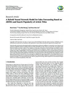
In this paper, we consider a neural network with two hidden layers, as shown in Fig. 1(a). The first hidden one is a sigmoid layer which maps the input features v into a binary representation h via a sigmoid function, i.e. h = σ(w1 v + b1 ) where σ(t) = 1/(1 + exp(−t)) and w1 , b1 are the parameters of this layer. The second hidden layer performs linear dimension reduction x = hw2 + b2 , with w2 , b2 being parameters. The output of the units x correspond to the transformation fw (v) provided the whole network. An arbitrary number of extra hidden layers could be inserted between these two layers if more a complex transformation is preferred. Let w = {w1 , b1 , w2 , b2 } denote all parameters of the network. Training the network is performed by back propagation [13] on w. The initialization of w is obtained by learning a Restricted Boltzmann Machine (RBM) [7] with the same structure of network. We will give details of the training procedure in section 3.2.

The hybrid model 2.2

Our hybrid model is a combination of one particular probabilistic model, hierarchical topic model (HTM), and a neural network (NN). We consider a set of N images {I1 , . . . , Ii , . . . , IN } with labels y. From each we extract a set of SIFT descriptors [15] {v1 , . . . , vj , . . . , vni }. Each descriptor vj is individually mapped by a neural network with parameters w to a feature vector xj in Rd , d being the number of units in the top layer of the network. The transformation of v → x is denoted by fw (v). The structure of neural network is encoded by layers of hidden units h. The connections of hidden units are given in section 2.1. Each image is represented by a topic model where each topic is a probability distribution over visual words in a vocabulary. In prevalent topic models such as LDA[4, 6] and its variants [21], the vocabulary is given by vector quantization, but not integrated into the topic model. In this paper, we want to learn the feature representation and the topic model jointly. We extend the topic model by adding an extra latent variable to encode visual vocabulary. Unlike other topic models, our model is directly defined over image features, and capable of learning vocabulary and topic distribution simultaneously. The new topic model is of hierarchical structure (see fig.1) whose distribution is given in section 2.2. The hierarchical topic model is combined with the neural network to form a hybrid model by treating the output x of the network as the bottom nodes of the hierarchy.

1288

Hierarchical topic model

Given an image Ii , the neural network will transform each raw feature vj into a vector xj , which is input to the hierarchical topic model. We assume that each xj is generated by a Gaussian distribution of the corresponding word cluster uj . The Gaussian is parametrized by φuj = {µuj , Σuj }. The word uj is generated by a multinomial word distribution with parameters of ηzj . The distribution of topics zj is a multinomial parametrized by πyi where yi is a label of scene category for image Ii . yi is provided in the learning stage. The overall model is shown in Fig. 1(b). The hierarchical generative process is given by: 1. Draw latent topic zj ∼ M ulti(πyi ) 2. Draw latent word uj ∼ M ulti(ηzi ) 3. Draw feature vector xj ∼ Gaussian(φuj ). The prior distributions on π, η, φ are defined as follows: πy ηz φu

∼ ∼

∼

Dir(α) for y ∈ {1, 2, . . . S} Dir(β) for z ∈ {1, 2, . . . M }

N IW(γ) for u ∈ {1, 2, . . . K}

where Dir(.) is Dirichlet distribution, N IW(γ) is normal-inverse-Wishart distribution, parametrized by γ = {µ0 , κ, ν, Λ0 }. S is the number of scene categories (class labels), M is the number of latent topics, and K is the size of word vocabulary.

Li Wan, Leo Zhu, Rob Fergus

α

π

β

η

γ

φ

S

M

u

Layer 4

Latent topic z M (=45) Integration F1 (η)

ni

Layer 3

Output x

(25 units)

Hidden units h

(a)

Feature x

Layer 2

(25 units)

Linear layer (W 2) (600 units)

Layer 1

Sigmoid layer (W 1) Input v

K (=200)

Latent word u Gaussian likelihood F2 (φ={μ,Σ})

Linear layer (W 2) Layer 1

S (=15) F1(π) Integration

N Layer 2

Bayes F0

Layer 5

z

x K

Class labels y

(b) (c)

y

Hidden units h

(600 units)

Sigmoid layer (W 1) 128d

Input v

128d

Figure 1: (a) Neural network (NN). (b) Hierarchical topic model (HTM). (c) Our hybrid model that combines the NN and HTM. The hyper-parameters α, β, γ are set by hand, their exact value not being too important. Learning the model involves the estimation of the parameters π, η, φ. In section 3.3, we will discuss the learning of the hierarchical model. Note that, unlike standard LDA[4], our model has no image (or document) specific prior of topic distribution. The most related representation is the scene model [21] which essentially is a author-topic model [18]. 2.3

The hybrid model: coupling the neural network and topic model

The hybrid model is designed to combine the strengths of the two models defined above. The input x to the hierarchical topic model is the transformed output fw (v) of the neural network. Note, in the hybrid model, x is not observable. The topic model captures high-level scene structure of an image while the neural network offers approximate low-dimensional embedding of raw features. Typically, the probabilistic topic model is a sparse graph while neural network is a densely connected graph.

3 3.1

input data v. The loss function is given by: L(w, π, η, φ) = − log p(y|v, w, π, η, φ)

(1)

Since x = fw (v), p(y|x, w, π, η, φ) = p(y|v, w, π, η, φ), and applying Bayes rule, we thus have: L = − log p(fw (v)|y, π, η, φ)+log

S X

p(fw (v)|˜ y , π, η, φ)

y˜=1

(2) The likelihood function of the hierarchical topic model for an image Ii is defined as p(fw (v)|y):   ni X K M X Y  p (fw (vj )|uj , φ) p (uj |zj , η) p (zj |y, π) j=1 zj =1

uj =1

The optimization of the loss function is performed by gradient descent. The learning procedure consists of two steps: 1. We first initialize the parameters {w0 , π 0 , η 0 , φ0 } obtained by pre-training the neural network and the hierarchical topic model which will be introduced in sections 3.2 and 3.3. 2. The parameters are then updated according to the following rules (where c is a learning rate):

Learning the hybrid model Brief description

The task of learning the hybrid model is to maximize the posterior distribution of class label y, given the

1289

wt+1

=

η t+1

=

∂L ∂L t+1 ,π = πt − c ∂w ∂π ∂L ∂L t+1 t t ,φ =φ −c (3) η −c ∂η ∂φ wt − c


The major technical issues of learning are (i) how to obtain a good initialization; (ii) how to calculate the gradients of the loss function defined over the joint model. We will address these two issues in the following sections. 3.2

Pre-training of neural network

We first pre-train the neural network by learning RBMs with the same structure in an unsupervised manner. A RBM is an undirected graphical model with connections between visible units v and hidden units h. The joint distribution p(v, h) ∝ exp(−E(v, h)) with the normalization constant Z = P exp(−E(v, h)). The transformation provided by v,h neural network is defined as p(h|v) in the corresponding RBM. We apply the contrastive divergence (CD) algorithm [7] to train the network. CD algorithm is a greedy layer-wise learning method for stack of Restricted Boltzmann machine (RBMs) which maximize the variational lower bound of the model likelihood. Hinton and Osindero [7] show that such initialization works well for discriminative training. Each layer of NN is initialized by the corresponding RBM model. More precisely, the RBM energy for pre-training of the bottom layer is E(v, h) = − 12 (v − b)T (v − b) − hT c − v T W h. The energy of RBM for pre-training of the second (top) layer is E(h, x) = − 21 (x − c)T (x − c) − hT b − hT W x. 3.3

foreach image i do foreach feature j do • Remove uij from the cached statistics for current latent variable k = zij and m = uij : πyk ← πyk − 1,ηkm ← ηkm − 1 and φm ← remove uij from φm . • Sample zij and uij jointly from the following multinomial distribution: p(zij , uij |xij , π, η, φ, α, β, γ) ∝ p(xij |uij , φ, γ)p(uij |ηzij , β)p(zij |πyi , α). • Add back feature xij to the cached statistic for its new latent variable k = zij and m = uij : πyk ← πyk + 1,ηkm ← ηkm + 1 and φm ← add uij to φm . end end Algorithm 1: Gibbs sampler for the hierarchical topic model.

takes an input of a matrix A and a label information y. F0 (A, y) is a form of: F0 (A, y) = −

Aji

= =

Joint optimization by gradient descent

=

Let F0 (A, y) ≡ L where A is a ni × S matrix, Aji = [p(fw (vj )|y = i, π, η, φ]ji and F0 is a function which

1290

(4)

M X

p(fw (vj )|zj , η, φ)p(zj |y = i, π)

[F1 (B, C)]ji

The decomposition of matrix B is given by: Bjm

= =

p(fw (vj )|z = m, η, φ) K X

uj =1

=

p(fw (vj )|uj , φ)p(uj |z = m, η)

[F1 (D, E)]jm where Djk = p(fw (vj )|u = k) and Ekm = p(uj = k|z = m, η)

p(fw (vj )|y = i, π, η, φ)

i=1 j

Aji

j

Here matrix B is of size ni × M and matrix C is of size M × S. Function F1 is a multiplication of two matrices, i.e. A = F1 (B, C) = BC.

j

log

i

where Bjm = p(fw (vj )|z = m, η, φ) and Cmi = p(z = m|y = i, π)

We now have the full pre-trained model with all parameters initialized. Gradient descent is applied to update the parameters. The loss function defined in Equation (2) can be expanded as follows: X L = − log p(fw (vj )|y, π, η, φ) + S Y X

j

XY

p(fw (vj )|y = i, π, η, φ)

zj =1

3.4

log Ajy + log

We can decompose each element of A as follows:

Pre-training of the hierarchical topic Model

Once we have pre-trained the neural network, the resulting x = fw (v) are fixed and used as input to the hierarchical topic model. The training of the graphical model is performed by Gibbs sampling in the style adopted by Sudderth et al. [21] in their similar scene model. The sampling procedure is given in Algorithm 1:

X

where E is the η matrix of size K × M and D is of size ni × K. We can decompose the matrix D: Djk

=

p(fw (vj )|u = k, φ)

Li Wan, Leo Zhu, Rob Fergus

1 T and |Σk |−1 exp − (fw (vj ) − µk ) Σ−1 (f (v ) − µ ) w j k K 2 ∂[F1 (B, π)]ik [F1 (B, π)]ik Bij − P =P = [F2 (x, φ)]jk where φk = {µk , Σk } ∂πjk t πjt t πjt P The reason that we divide the output by k Rjk Function F2 evaluates the likelihood (dropping out is because the second parameter π of this function the normalization constant) of the input data vi is always sufficient static of multinomial distribufor different Gaussian centers φk = {µk , Σk } for tion, thus must always sum to one. The derivative k = 1, 2, . . . , K. The output of F2 (fw (v), φ) is for F1 (D, η) takes a similar form. |Σk |−1 exp(− 1 (fw (vj ) − µk )Σ−1 (fw (vj ) − µk )T ). =

k

2

After defining the functions F0 , F1 , F2 , the loss function can be rewritten: D

C E }| { z}|{ z z}|{ L = F0 (F1 (F1 (F2 (fw (v), φ), η ), π ), y) {z } | B | {z }

(5)

3. Function F2 (x, φ) ,where φ = {φ1 , φ2 , . . . , φK } each of φk is a Gaussian center φk = {µk , Σk } [F2 (x, φ)]jk = |Σk |−1 exp(− 12 (xj − µk )Σ−1 k (xj − µk )T ) Taking gradients we obtain (omitting the Σk update for brevity): ∂[F2 (x, φ)]jk ∂xj ∂[F2 (x, φ)]jk ∂µk

A

and

∂L ∂π ∂L ∂η ∂L ∂φk

=

∂L ∂w

=

=

=

∂F0 (A, y) ∂F1 (B, π) ∂A ∂π ∂F0 (A, y) ∂F1 (B, π) ∂F1 (D, η) ∂A ∂B ∂η ∂F0 (A, y) ∂F1 (B, π) ∂A ∂B ∂F1 (D, η) ∂F2 (fw (v), φ) ∂D ∂φk ∂F0 (A, y) ∂F1 (B, π) ∂F1 (D, η) ∂A ∂B ∂D ni X ∂F2 (fw (vj ), φ) ∂fw (vj ) ∂fw (vj ) ∂w j=1

3.5

The gradients of L w.r.t w, φ, η, π can be obtained by applying chain rule, provided the gradients of F0 , F1 , F2 : 1. Function F0 (A, y) evaluation: F0 (A, y) = −

X

log Ajy + log

ni S Y X

Aji

[F2 (x, φ)]jk (xj − µk )Σ−1 k

Unifying probabilistic hierarchical model and neural network: back-propagation

The gradient descent scheme introduced in section 3.4 can be interpreted as a back-propagation algorithm on a new neural network which unifies the hierarchical topical model and the neural network. The decomposition of the loss function in Equation (5) allows us applying chain rule to calculate the gradients w.r.t. all the parameters in the hybrid model. It suggests a strong connection with the back-propagation algorithm if we define four consecutive layers from top to bottom in the following order: 1. Bayesian Layer: Function F0 2. Integration Layer on z: Function F1 with π as the second parameter

The transformation of each layer is defined by the corresponding function F and its parameters. We can simply add these four invented layers on the top of the original neural network, yielding a unified neural network. By back-propagating through this unified network, we can estimate the parameters of the hybrid model.

exp(F0 (A, y)) ∂F0 (A, y) = −1 + Aji Aji 2. Function F1 (B, π) evaluation: P and gradient computation:

=

4. Gaussian Likelihood Layer: Function F2

and gradient computation:

[F1 (B, π)]ik =

−[F2 (x, φ)]jk (xj − µk )Σ−1 k

3. Integration Layer on u: Function F1 with η as the second parameter

i=1 j=1

j

=

j Bij πjk P k πjk

3.6

Inference of the hybrid model: feed-forward

Inference is performed as a feed-forward procedure on the unified neural network. Given a testing image v,

πjk ∂[F1 (B, π)]ik =P ∂Bij t πjt

1291


the first two layers of the neural network produce encoded features x = fw (v). According to the definition of the four additional layers, the output at the top layer is p(y|fw (v)) for y = 1, 2, . . . , S. The task of inference y ∗ = arg maxy p(y|fw (v)) is the same as passing x through Gaussian likelihood layer(F2 ), Integration layer(F1 (·, η)), Integration layer(F1 (·, π)) and Bayesian layer F0 (see Figure 1(c)). Note that our hybrid approach can be extended to any graphical model where the (approximate) inference can be performed in closed-form.

4

Toy experiments

We illustrate the different stages of training in our model with toy 2D data, as shown in Figure 2. The data is drawn from 4 classes, arranged in 5 crescentshaped clusters (which cannot easily be separated by a Gaussian mixture model). Pre-training the NN (having a 2-50-2 architecture) for the most part preserves the structure of the input data (see Figure 2(middle)) in the feature space, thus the topic model, using Gaussian distributions makes many classification errors. But following back-propagation of the entire model (Figure 2(right)), the NN provides a significant warping of the input space, thus making it easier to separate the clusters. Note that the Gaussian clusters of the topic model do not lie directly on top of the features since the topic model optimizes a discriminative criterion, rather than a generative one.

5

Vision experiments

In this section, we provide a quantitative evaluation of our hybrid model on a vision dataset and compare its performance with alternative methods such as a standard neural network, hierarchical topic model, pLSA, LDA and their variants. 5.1

Dataset and image features

We evaluated our hybrid model on challenging image scene recognition dataset [12] where the experimental results of standard probabilistic graphical models such as pLSA and LDA have been reported. This dataset consists of 1500 training images and 2998 test images each of which is labeled by one of 15 scene categories such as street, kitchen, coast, etc. Each image is represented by a set of SIFT descriptors which are sampled every 16 pixels (giving ∼ 240 per image). Each SIFT descriptor is a 128-dimensional vector which encodes the histogram of gradients of a local image patch with size of 32 × 32. Since we focus on the theoretical issues involved when combining NN with graphical models, the pyramid representation [12] which leads to better

1292

performance is not used. 5.2

Scene modeling: topic model, neural network and the hybrid

Topic model. The baseline model of image scene is standard LDA [4, 6]. We first form visual vocabulary with size of 200 (following [6]) where visual words are obtained by vector quantization of SIFT descriptors. An image scene is represented by LDA which learns the latent topic distributions of visual words. When labels are provided in training, the variants of LDA such as supervised LDA [3] and discriminative LDA [11] can be applied. The performance of LDA is directly based on [6]. Hierarchical topic model. Unlike LDA, the hierarchical topic model introduced in section 2.2 integrates the representation of dictionary. The observation data input to HTM is SIFT features. The HTM is capable of learning the visual vocabulary and the topic distribution jointly. Our HTM method which makes use of class labels is related to the discriminative version of LDA [11]. We also follow the standard way [12, 11] to study the discriminative power of the inferred latent topics by training a SVM with the assigned topics as classification features. Note that the input to all variants of both HTM and LDA models are fixed visual vocabulary without the ability of learning transformation of low-level feature representation, i.e. SIFT descriptors. Neural network. We use the same architecture of the neural network as described in section 2.1. In order to predict scene labels, we extend the neural network by imposing a softmax layer on the top which performs logistic regression of the scene labels and the output of the feature transformation. Learning the extended neural network is performed by standard backpropagation [13]. Unlike the topic models, this approach lacks a high level model of the scene. Hybrid model: The hybrid model is a combination of the hierarchical topic model and the neural network which integrate the ability of learning lowlevel feature transformation and high-level scene representation. The input to the model is SIFT features, used by the other approaches. The free parameters and hyper-parameters are set to S = 15 (categories), M = 45 (topics), K = 200 (words), α = 1/3, β = 1/3. Let d denote the dimension of µ (=25). γ is set to (µ0 = 0d , κ = 0.1, ν = d + 5, Λ0 = Id ). The NN has a 128 − 600 − 25 architecture. Back-propagation is performed using conjugate gradients, with mini-batches of 75 images by ∼ 200 features/image. Convergence occurs in about 70 iterations. The corresponding separate HTM and NN use the same parameter settings.

Li Wan, Leo Zhu, Rob Fergus 15

Input v

Features x 6

8

(Before Backprop)

10

Features x (After Backprop)

6 4 4

5 2

2 0 0

0

−2

−2

−5

−4 −10

−4 −6

−15 −5

−6 −4

−3

−2

−1

0

1

2

3

4

5

−8

−6

−4

−2

0

2

4

6

8

−10

−8

−6

−4

−2

0

2

4

6

8

Figure 2: Toy experiment using 2D data (left), with 5 clusters drawn from 4 classes (cross, dot, square, circle). Note that there are multiple clusters per class. Middle: Visualization of 2D feature space x after NN pre-training and Gibbs sampling of supervised topic model with K=5 clusters and Y=4 classes. The ellipses show the mean and covariance of each Gaussian cluster in the HTM. In the HTM, the color indicates the predicted class of each data point (the labels: red=cross, green=dot, blue=square, cyan=circle). Note that several points are mislabeled. Right: The feature space after back-propagation of unified model. The NN has distorted the feature space to make classification easier for the topic model, with only a single data point now being misclassified.

pLSA+SVM [12] 63.3 HTM+ SVM 65.5 ± 1.5

LDA [6] 65.2 Hybrid model no pre-train 47.2

Supervised LDA [3] 67.0 Hybrid model pre-train NN only 52.5

Neural Network 51.6 ± 1.1 Hybrid model pre-trained 65.7 ± 0.4

HTM 64.9 ± 1.2 Hybrid model fully trained 70.1 ± 0.6

Table 1: Classification rates of our model and other approaches on a scene classification dataset [12]. Our implementation of discriminative hierarchical topic model (HTM) is similar to Sudderth’s scene model[21]. The performance of the HTM alone is close to the other two probabilistic models (pLSA+SVM) reported in [12] and discriminative LDA [6] which is evaluated on 13 categories. The method of “HTM+SVM” is a multi-class SVM with the input features of the latent topic assignments of HTM. Our hybrid model is a combination of neural network and HTM. We report the results of both pre-training and joint optimization, with the latter achieving a performance of 70.1%.

5.3

Results

We report the classification accuracy of the three types of methods in Table 1. Each model is trained on 5 random splits of training and test sets. We can see that the neural network, which lacks high-level representation, performs badly with classification accuracy of 51.6%. We also tried adding an extra hidden layer to better match the capacity of hybrid model, which resulted in a performance of 50.7%. The baseline HTM achieves 64.9% which is significantly better than neural network, and is comparable with other latent topic models LDA [6] (65.2%) and pLSA [12] (63.3%). The method of “HTM+SVM” which is a multi-class SVM using latent topic assignments of HTM as classification features, provides slightly improved predictions (65.5% vs 64.9%). The hybrid model is analyzed after: i) pre-training and ii) full training with joint optimization. The pretrained hybrid model achieves 65.7% , slightly better than HTM, which shows that simple pre-trained feature transformation offers similar predictions. The fully trained hybrid model further improves the classi-

1293

fication accuracy to 70.1% which is significantly better than HTM. It shows that joint optimization is capable of learning better low-level feature transformations for high-level topic modeling.

6

Discussion

We have introduced a unified representation that unifies two distinct classes of model that are widely used in machine learning and an end-to-end training scheme for the model. A number of improvements to our model could easily be incorporated. For example, a convolutional form of NN [13] could be used to directly learning from image pixels, or a spatial structure could be incorporated into the topic model, in the style of Sudderth et al. [21]. Our approach for joint training of the two models is a simple one that can be applied to more complex types of graphical model, provided (approximate) inference is possible in closed form. Finally, our model is not limited to image data and could easily be applied to other modalities such as text or audio.


References [1] R. P. Adams, H. M. Wallach, and Z. Ghahramani. Learning the structure of deep sparse graphical models. Journal of Machine Learning Research Proceedings Track, 9:1–8, 2010. [2] Y. Bengio, P. Lamblin, D. Popovici, and H. Larochelle. Greedy layer-wise training of deep networks. In In NIPS, 2007. [3] D. Blei and J. McAuliffe. Supervised topic models. In NIPS, 2007. [4] D. Blei, A. Ng, and M. Jordan. Latent Dirichlet allocation. Journal of Machine Learning Research, 3:993–1022, 2003. [5] C. Dance, J. Willamowski, L. Fan, C. Bray, and G. Csurka. Visual categorization with bags of keypoints. In ECCV International Workshop on Statistical Learning in Computer Vision., Prague, 2004. [6] L. Fei-Fei and P. Perona. A bayesian hierarchical model for learning natural scene categories. CVPR, pages 524–531, 2005. [7] G. E. Hinton and S. Osindero. A fast learning algorithm for deep belief nets. Neural Computation, 18:2006, 2006. [8] G. E. Hinton and R. R. Salakhutdinov. Reducing the dimensionality of data with neural networks. Science, 313(5786):504–507, July 2006. [9] T. Hofmann. Unsupervised learning by probabilistic latent semantic analysis. In Machine Learning, page 2001, 2001. [10] K. Kavukcuoglu, P. Sermanet, Y. lan Boureau, K. Gregor, M. Mathieu, and Y. Lecun. Learning convolutional feature hierarchies for visual recognition, 2010. [11] S. Lacoste-Julien, F. Sha, and M. Jordan. Disclda: Discriminative learning for dimensionality reduction and classification. In NIPS, 2009. [12] S. Lazebnik, C. Schmid, and J. Ponce. Beyond bags of features: Spatial pyramid matching for recognizing natural scene categories. In CVPR, pages 2169–2178, 2006. [13] Y. LeCun, L. Bottou, Y. Bengio, and P. Haffner. Gradient-based learning applied to document recognition. IEEE, 86(11):2278–24, 1998. [14] H. Lee, R. Grosse, R. Ranganath, and A. Y. Ng. Convolutional deep belief networks for scalable unsupervised learning of hierarchical representations. In ICML, pages 609–616, 2009. [15] D. Lowe. Distinctive image features from scaleinvariant keypoints. International Journal of Computer Vision, 60(2):91–110, 2004.

1294

[16] J. Ngiam, Z. Chen, P. W. Koh, and A. Ng. Learning deep energy models. In L. Getoor and T. Scheffer, editors, Proceedings of the 28th International Conference on Machine Learning (ICML-11), ICML ’11, pages 1105–1112, New York, NY, USA, June 2011. ACM. [17] M. Ranzato and G. Hinton. Modeling pixel means and covariances using factorized thirdorder Boltzmann Machines. In CVPR, 2010. [18] M. Rosen-Zvi, T. Griffiths, M. Steyvers, and P. Smyth. The author-topic model for authors and documents. In Uncertainty in Artificial Intelligence 20, pages 487–494, 2004. [19] R. Salakhutdinov and G. E. Hinton. Using deep belief nets to learn covariance kernels for gaussian processes. In NIPS, 2008. [20] R. Salakhutdinov, J. Tenenbaum, and A. Torralba. Learning to learn with compound hd models. In NIPS, 2011. [21] E. Sudderth, A. Torralba, W. Freeman, and A. Willsky. Describing visual scenes using transformed objects and parts. Intl. Journal of Computer Vision, 77, March 2008.